Correlation of fighter aircraft performance with combat effectiveness in a tactically significant environment

CORRELATION OF FIGHTER AIRCRAFT PERFORMANCE WITH COMBAT EFFECTIVENESS IN A TACTICALLY SIGNIFICANT ENVIRONMENT

by

ROBERT D. KOSCIUSKO

Submitted to the Department of Aeronautics and Astronautics in Partial Fulfillment of

the Requirements for the Degree of MASTER OF SCIENCE IN AERONAUTICS AND

ASTRONAUTICS at the

MASSACHUSETTS INSTITUTE OF TECHNOLOGY June 1991

@

Draper Laboratory of Author:

Department of Aeronautics and Astronautics, 3 June 1991 Approved by:

Martin V. Boitz Technical Supervisor, CSDL Certified by:

Professor Walter M. Hollister Department of Aeronautics and Astronautics Thesis Supervisor Accepted by:

Profes--- Harold Y. achman Professhr Harold Y. Wachman Chairman,

Aero

Departmental Graduate Committee

ViAQ_ýACtUSETSSINSTINUTE OF rECHNOLOGY JUN 1

1991

I ---

---

-Acknowledgement

This report was prepared at the Charles Stark Draper Laboratory, Inc. under Independent Research and Development Project 276, Connectionist Systems and Learning Control.

Publication of this report does not constitute approval by the Draper Laboratory of the findings or conclusions contained herein. It is published for the exchange and stimulation of ideas.

I hereby assign my copyright of this thesis to The Charles Stark Draper Laboratory, Inc., Cambridge, Massachusetts.

Permission is hereby granted by The Charles Stark Draper Laboratory, Inc. to the Massachusetts Institute of Technology to reproduce any or all of this thesis.

Robert D. Kosciusko

I wish to thank all the individuals who have contributed to my success in completing this thesis. In particular, I am indebted to B. Gable for providing invaluable technical assistance for all portions of the study. M. Boelitz was the motivating force who secured financial support from CSDL in order to complete the IR & D effort. I would like to express my sincere gratitude to both of you for going out of your way to ensure that I received professional guidance and assistance throughout all stages of my graduate study. The Draper Fellowship has provided the means to acquire such a rich educational experience.

In addition, I thank my thesis supervisor, Prof. W.M. Hollister. Your overwhelming technical expertise combined with your

experiences in naval aviation have conveyed unto me a sound

foundation of knowledge which I used to direct the research efforts. I give special thanks to my parents. Their enthusiasm and love have been felt steadily through the years.

Correlation of Fighter Aircraft Performance with Combat Effectiveness in a Tactically Significant Environment

by

Robert D. Kosciusko

Submitted to the Department of Aeronautics and Astronautics on June 3, 1991 in partial fulfillment of the

requirements for the Degree of Master of Science in Aeronautics and Astronautics

ABSTRACT

Five measures of effectiveness have been defined to compare two aircraft models flying simulated combat engagements. The autonomous vehicles were controlled by improved versions of the original Adaptive Maneuvering Logic pilot developed by NASA's Langley Research Center. One of the combating aircraft was given propulsive and aerodynamic advantages over the baseline F-18 aircraft. Both aircraft were flown by the same pilot logic. The

results indicate that some advantages translate directly to increased combat performance while others do not. Normal acceleration was found to be the most important quality of the maneuvering fighter. To improve an aircraft such that it acquires a sizeable fighting advantage over the baseline F-18, it is necessary to provide the aircraft with normal accelerations and g ratings beyond human physiological limits.

Company Supervisor: M. Boelitz

Thesis Supervisor: Professor W.M. Hollister Title: Professor of Aeronautics and Astronautics

CONTENTS

1. INTRODU CTION ... 1

2. ABOUT THE COMBAT SIMULATION...3 2.1 The AML "Pilot"... ... 4 2.2 The F-18 Aircraft Model and the Implementation of

Performance Advantages...6

2.3 Effectiveness Parameters and the Weapons

E nvelope ... ... 9 2.4 Initial Geometries For Simulated Engagements ... 12

3. A NEW THRUST CONTROL STRATEGY... 15 3.1 Shortcomings of Old Logic... ... 1 5

3.2 A Modified Bang-Bang Controller... 5

3.3 Thrust Controller Comparisons ... 1 9 4. R E SU L T S ... 2 1

4.1 Correlation of Effectiveness Parameters with Load

Factor A dvantage ... 2 1 4.2 Correlation of Effectiveness Parameters with Thrust

A d v an tag e ... ... 2 7 4.3 Correlation of Effectiveness Parameters with Speed

B rake A dvantage ... 3 3 4.4 Correlation of Effectiveness Parameters with

Combined Advantages... 37

5. DEPENDENCE OF AIRCRAFT EFFECTIVENESS ON ENGAGEMENT

IN ITIA L CON D ITION S ... 4 1 6. C O N CLU SIO N ... 4 7 7. B IBLIO G RA PH Y ... 4 9

I

LIST OF FIGURES

Figure Page

1. Attacker vs. Target Trajectories 4

2. Dissimilar Aircraft Trajectories 8

3. Deviation Angle and Angle Off (AOT) 1 1 4. State Variable Diagram of Controller 17

5. Diagram of the Variable Xtina 18

6. Guns Time vs. G Multiplier 21

7. Offense Time vs. G Multiplier 22

8. TOA vs. G Multiplier 22

9. Scatter Plot of Guns Time with Linear Regression 23 10. Guns Time vs. G Multiplier (Over wider range) 25 11. _{Offense Time vs. G Multiplier (Over wider range) 25} 12. TOA vs. G Multiplier (Over wider range) 26

13. Guns Time vs. Thrust Advantage 27

14. _{All-Aspect Missile Lock Time vs. Thrust Advantage 2 8} 15. Number of Kills in 50 Engagements vs. Thrust Advantage 2 8 16. Scatter Plot of Number of Kills with Linear Regression 29

17. Maximum Thrust Time Histogram 30

18. 3-D Military/Afterburner Thrust Histogram 3 1 19. Average Time at Throttle Position (500 engagements) 3 2 20. Guns Time vs. Speed Brake Advantage 3 4

21. TOA vs. Speed Brake Advantage 34

22. Number of Kills vs. Speed Brake Advantage 3 5 23. Scatter Plot of Number of Kills with Linear Regression 3 6 24. 3-D Plot of Offense Time vs. Thrust and G Advantages 3 8 25. 3-D plot of Number of Kills vs. Thrust and G Advantages 3 9

26. Guns Time vs. Range 42

27. Offense Time vs. Range 43

28. All Aspect Missile Time vs. Specific Energy 44 29. TOA vs. Initial Heading Difference 45

LIST OF TABLES

Tables Page

1. Linear Regression Analysis for G Advantage 24 2. Linear Regression Analysis for Thrust Advantage 29 3. Linear Regression Analysis for Speed Brake Advantage 35

As new technologies are proposed for inclusion in high-performance fighter aircraft, it becomes imperative to assess the utilization and impact of these capabilities within the context of air-to-air combat. Without the use of a realistic simulation however, the determination of the worthiness of a technological advancement in

fighter aircraft can only be found after building and flying the plane in a combat arena. Even if this were to be done, it is difficult to quantify the relative effectiveness of the combating aircraft and

even more difficult to separate the contributions in effectiveness between the better aircraft and the better pilot.

A simulation allows two aircraft to be flown by the same automated pilot, thus permitting any advantages in combat to be attributed only to performance of the plane instead of performance of the pilot. Although this was not the original intent of the early combat simulations designed by NASA, their latest algorithm, developed for autonomous vehicle guidance in combat scenarios, serves the purpose well. The AML, short for Adaptive Maneuvering Logic, was created to guide an autonomous fighter aircraft against another aircraft flown by another algorithm or a human. This study uses the AML as a tool for testing different aircraft in an integrated hostile environment, one that is both controllable and repeatable.

The AML, using its three degree-of-freedom aircraft model for the F-18, is flown against itself to test some advanced flight

characteristics not possible in today's fighters. By varying the characteristics, the advantages or drawbacks of a superior performance vehicle are explored.

As an example of the worth of such a study, note that

expanding the flight envelope in certain regions has been shown to be beneficial in combat. The F-16's ability to pull nine g's instead of an F-4's six or seven has made it the superior fighter. This study attempts to determine if continually enhancing the performance of a fighter, perhaps through aerodynamic and propulsive improvements and human factors research, necessarily furthers the superiority of

II

m

the plane in combat. If this is so, it should be possible to suggest the technologies required to make fighters more effective and to predict, due to the vehicle accelerations, whether or not humans will be a part of the combat process.

Fighter aircraft are customized by varying three translational performance parameters in one of two simulated F-18's. The

maximum g limit, maximum afterburner and military thrust

attainable by the engine, and the maximum drag produced by speed brakes are the modified characteristics. The target aircraft retains the baseline F-18 characteristics. The advanced configuration fighter is deemed the attacker.

For each new configuration attacker, fifty close-in combat engagements with random initial geometries are simulated. The

same automated AML "pilots" fly both the target and the attacker planes so that the advantages perceived are due only to the aircraft. Five measures of effectiveness are employed to quantify one

aircraft's dominance over the other. The metrics, averaged over fifty engagements, are correlated with the attacker's performance

capabilities. Based upon the attacker's performance, it is possible to reach a conclusion as to which aircraft improvements translate

directly to improvements in combat effectiveness.

In addition to this, a further study attempts to determine the dependence of the effectiveness measures on the engagement initial conditions. Both the attacker and target are given the F-18 baseline configuration and the engagement scoring is correlated with each aircraft's initial geometry advantages.

The AML is a real-time digital computer program that operates a fighter plane interactively against an opponent. The opponent may be another AML pilot, or a human pilot in simulated combat. The FORTRAN program makes maneuvering decisions from typical on-board sensors and instruments found on any fighter aircraft, and a continuous knowledge of the opponent's relative position. The code was first written by the Langley Research Center to include an F-4 model. The tactics and decision logic have been modified to a great extent since then by the Charles Stark Draper Laboratory. The baseline aircraft model has also been changed to that of the F/A-18 Hornet.

The combat environment consists of an unlimited region of airspace above flat land of zero elevation. The planes may maneuver over the entire region as far and as high as their engines will carry them. _{Through a sixty-second engagement, the aircraft will usually}

stay within a 100 square mile area. The initial conditions of the engagement are kept within a 25 square mile area such that close-in one-on-one air combat may be simulated. Throughout the

engagement, each aircraft is scored on its effectiveness. Figure 1 displays a plot of an engagement run by the simulation with similar aircraft, similar pilots, and symmetrical initial conditions. There is a ground trace of the trajectories in order to facilitate visualization of the fight.

m

m

60 Second Engagement With Similar Aircraft And Equal Pilots

Symmetric Initial Conditions

Figure 1: Attacker vs. Target Trajectories

2.1 The AML "Pilot"

The AML "pilot" consists mainly of a maneuver selection logic which outputs a commanded bank angle, throttle setting and load level to the aircraft model. It does this by first predicting its

opponents position two seconds from the present time using a linear extrapolation. The code then selects several trial maneuvers and integrates to predict what its own state will be after the same two seconds have elapsed. The computed state at the end of each of the optional maneuvers is compared with the predicted state of the opponent using a weighted decision logic. This is done by asking

m

several questions about the states involving quantities such as positions, angles, velocities, and distances. The first question, for example, asks whether the target will be in front of the attacker at the end of the 2-second period for each of the trial maneuvers. After the answers to each of the questions is weighted by a user-defined array of parameters, the state comparison is provided a score by which the trial maneuvers can be evaluated. The trial with the

highest score is then considered the most promising maneuver and is executed next.

The program pilot selects several standard trial maneuvers depending on its assessment of its current tactical situation. As an example, one of the trials will involve rolling into the plane

containing the attackers velocity vector and the targets position and flying the trajectory for intersection. Special maneuvers are also incorporated to handle ground avoidance and energy management. Questions regarding ground avoidance are given a much higher weighting especially if a maximum g pull-up is required to prevent contacting the ground. In addition, the aircraft will very often not use its full load factor capability due to energy management

considerations. If it determines that it will gain a satisfactory

advantage by using a trial maneuver with the maximum load factor, however, it will not hesitate to use the aircraft's full potential.

For most situations, the AML will use lag pursuit rather than higher risk lead maneuvering. The degree of lag or lead pursuit can be easily modified by changing the target extrapolation interval. If lead is employed all of the time, the target may be able to capitalize on this and alter his trajectory to put the attacker in a disastrous situation.

Combining all of these ideas, the AML is a formidable pilot. In fact, at the Langley Differential Maneuvering Simulator (DMS), the AML has competed against highly-trained U.S. Air Force and Navy fighter pilots in real time. The DMS permits the human pilots to maneuver their aircraft in a 360 degree dome with projected

imagery for a one-on-one combat simulation. Although it is difficult to define clear-cut win-loss criteria for simulated air combat

AML pilot had significantly more time on the offense than did the military pilots opposing it. In most of the engagements, the AML received greater overall scores than the human pilots who flew

against it. For close-in one-on-one combat, the AML has been shown to be a suitable pilot for the purposes of this study.

2.2 The F-18 Aircraft Model and the Implementation of Performance Advantages

The AML uses a three degree-of-freedom model of the F/A-18.1 The plane may be rotated about the longitudinal axis (roll), accelerated along the longitudinal axis, or rotated about the lateral axis (pitch). The AML pilot reacts to information presented to it through simulated instrumentation to output a commanded bank angle, load level, throttle setting, and speed brake deflection. These are inputs to the aircraft model. The equations of motion are then used to compute the state of the aircraft. The equations of motion consist of both force and moment equations that use tabulated aerodynamic derivatives which define the aircraft being flown. By modifying these derivatives, the aircraft's performance capabilities may be changed.

In order to produce attacker aircraft with more performance than the F-18 target, the model derivative data was changed so that advantages in lift, drag, and acceleration due to thrust could be obtained. First, the tables for the models are used to evaluate the thrust produced by each engine as a function of Mach number and altitude. Afterburner thrust data may be modified separately from military thrust at certain Mach numbers or altitudes, thus enabling different performance regimes of the engine to be enhanced. The numbers are varied individually for the attacker by multiplying the baseline table by some factor of improvement. As an example, a thrust factor of 1.1 provides the attacker a ten percent increase in thrust over the baseline F-18 model.

1 A more detailed description of the aircraft model may be found in the

documentation for the original computer simulation listed in the bibliography of this report: An Adaptive Maneuvering Logic Computer Program for the Simulation of One-on-One Air-to-Air Combat, Vol I and II, [2].

Similarly, the attacker is provided an enhanced lift capability by increasing CLmax. Again, a factor of 2.0, for instance, will

represent a doubling of the baseline configuration maximum coefficient of lift. The maximum speed brake drag is modified by multiplying the coefficient of drag of the deflector by a factor as the coefficient is read from a table.

For each sixty second engagement, the multipliers along with other performance data are recorded in a results file in the following order: _{initial conditions for the engagement, maximum load factor} multiplier, thrust factor multiplier, speed brake drag multiplier, and the airplane effectiveness parameters to be discussed later. This system is effective because only three parameters are necessary to describe complex overall aircraft system improvements. These three parameters are correlated with the attacker's effectiveness in

combat.

Figure 2 displays two aircraft trajectories. The one beginning on the left is the target. The aircraft on the right, the attacker, has double the thrust and double the maximum load factor of the target. It is evident from the plot that the attacker is able to maneuver himself behind the target for a close-in weapons delivery.

60 Sec Engagement With Dissimilar Aircraft And Equal Pilots

Symmetric Initial Conditions 2x Thrust Advantage plus 2x G advantage

Figure 2: Dissimilar Aircraft Trajectories

In order to program the model modifications, assumptions were made regarding the performance advantage implementations. First, it was assumed that the advanced aircraft simulated by the attacker model was designed to be structurally sound enough to handle the increased loads. _{Second, no disturbing moments were} generated by increasing the speed brake drag. Finally, the attacker did not require additional spool-up time for the engine to attain its increased thrust levels. Nonetheless, an attempt to maintain a

|

likeness to realism was made. As an example, the speed brakes require a finite time to achieve full deflection. The instantaneous coefficient of drag due to the speed brakes varies proportionally with their deflection angle.

With these aircraft performance enhancements, care had to be taken to ensure that the range of parameter modifications were kept such that the performance given to the attacker aircraft did not exceed that guidable by the present decision logic in the AML. The concern was that, since pilot tactics were written for approximately equal aircraft, the logic may not guide the attacker aircraft to employ its full potential. _{In order to prevent this, the range of parameter} modifications were kept within reasonable bounds and some

modifications were made to the decision logic. As an example, when the initial simulation model was given a factor of 2.0 thrust

advantage, the attacker aircraft lost because the existing thrust control logic was not able to support the advantage. The attacker accelerated right past the target when it should have attempted to station-keep behind it. Because of this, a new bang-bang thrust controller, described later, was installed in both the target and attacker aircraft pilot's logic. Even with the new logic, extreme thrust advantages posed problems for the computer pilot. As a further example, studies run with a maximum load factor multiplier greater than three showed that the attacker did not utilize his load level advantage. _{One must realize, however, that if the target F-18 is} capable of pulling 9.0 g's, a factor of 3.0 represents an attacker

capable of 27.0 g's. Even future aircraft will not be capable of supporting this load structurally. Simply put, the performance advantages must be kept within reasonable bounds.

2.3 Effectiveness Parameters and the Weapons Envelope

Because air combat maneuvering is complex, no single

performance index has been found which measures the outcome of one-on-one simulated air combat. In light of this, several different figures of merit were used to evaluate the outcomes of the

engagements. _{These are: time in guns envelope, time in missile lock,}

10

time on offense, time on offense with advantage, and first aircraft in the weapons envelopes (defined as a kill.) Some, such as time on offense with advantage, were deemed more worthy indicators than others based upon close examination of the fights. Each parameter will be defined separately.

Time in Guns

An aircraft was credited with time in guns for the amount of time it could remain within 5000 feet of the opponent and

simultaneously keep its nose within 5 degrees of the foe. This

translates to requiring the aircraft's deviation angle2 _{to be less than}

5 degrees.

Time in All Aspect Missile Lock

The missiles on board each aircraft were assumed to be AIM 9L all-aspect Sidewinders. In order to be credited with time in missile lock, the opposing aircraft had to remain inside the missile envelope for at least three seconds to attain the "lock". If three consecutive seconds are achieved, the time in missile lock begins accumulating. _{The missile envelope requires the aircraft to be at} least 3,000 feet from the opponent but have a range not greater than 30,000 feet. In addition, the aircraft must keep the opponent within 15 degrees of its own nose. In other words, the deviation angle must be less than or equal to 15 degrees.

Time on Offense

The time on offense is a general effectiveness parameter which roughly indicates the amount of time that the aircraft in question is chasing the opponent. Mathematically, the envelope is defined by requiring that the aircraft keep its own deviation angle less than 60 degrees while, at the same time, keeping the angle off the opponents tail (AOT) less than 60 degrees. Figure 3 helps to describe the

relative geometries.

2 _{The deviation angle of an aircraft is the angle between the airplane's own} velocity vector and the line of sight (LOS) to the opponent. The line of sight (LOS) is the line connecting the two aircrafts' centers of gravity.

Attacker _{Line of Sight Target}

(LOS)

Figure 3: Deviation Angle and Angle Off (AOT) Time on Offense With Advantage

The time on offense with advantage (TOA) is slightly different from basic time on offense. It is the most widely used parameter to evaluate the AML at the Langley Differential Maneuvering Simulator. TOA is defined as the time that the aircraft is behind the opponent and the opponent is in front of the aircraft. It is the accumulated time that one airplane is able to keep its opponent in front of its wing line and simultaneously remain behind the opponent's wing line. Mathematically, this translates to keeping the deviation angle less than 90 degrees while the angle off (AOT) is kept under 90 degrees as well. It is calculated much like the time on offense, but the requirements are relaxed by thirty degrees. Although this parameter covers a wide range of conditions, from close-in tracking to long range parallel flight, it has proven an excellent indicator of relative maneuvering performance in the past. Many real-time

differential maneuvering simulations with human pilots attest to this fact.

The four figures of merit are to be correlated with airplane performance advancements. _{One most note, however, that there are}

actually eight parameters: four statistics for the attacker and four for the target. In order to simplify the correlations, these eight were combined into four by subtracting the targets accumulated time from the attackers accumulated time for each of the effectiveness

parameters. The final four statistics were renamed: Guns Time, All-Aspect Time, Offense Time, and Offense Time With Advantage. They are each computed as the difference between the respective

le Off

)T)

effectiveness parameters of the attacker and the target. If the parameter has a value of zero, this indicates that the time for the target was the same as the time for the attacker. A value of zero is to be expected if similar aircraft with similar pilots are flown against each other with symmetrical initial conditions. Likewise, if the value is negative, this will indicate that the target faired better according to that particular measure of effectiveness. This system works well for the study because the attacker will have been provided a

performance advantage in most cases. One would expect that he should then out-perform the target and force most of the parameters to be greater than zero, or positive.

Kill Indicator

The kill indicator is the fifth measure of the aircraft's

effectiveness. It is slightly different than the others in that it is not an accumulated amount of time. Rather, the kill indicator is a flag with three discreet possible values for each engagement: -1, 0, or 1. A negative one (-1) is assigned to an engagement if the attacker was the first aircraft to be in either of its opponent's two weapons

envelopes: guns or missile lock. In other words, the target kills the attacker. Similarly, a positive one (+1) is assigned if the target is the first to be in either of the attacker's weapons envelopes during the

sixty second engagement. In this case the attacker kills the target. Finally, the zero is assigned if either both planes entered the other's envelopes at exactly the same time, or neither of the planes was able to use their weapons on each other. The kill indicator is a parameter which can roughly be used to determine who wins the fight.

A total of five effectiveness parameters are used to evaluate the attacker's advantages in combat. These are: Guns Time, All-Aspect Time, Offense Time, Offense Time With Advantage, and the number of kills.

2.4 Initial Geometries For Simulated Engagements

Initial conditions for each sixty second engagement had to be specified at the beginning of each run. Both aircraft could be given any initial position, velocity, altitude, and heading. Though similar

aircraft with similar pilots should have effectiveness parameters near zero, under certain initial conditions one aircraft could be favored over the other. Advantages of this type can be in the form of relative position or energy. In this study, it was necessary to factor out the advantage given a plane by the initial geometries so that any combat effectiveness perceived could be attributed only to advanced performance. There were two ways in which this was done.

First, for each case of a specific vehicle advantage (maximum load factor, thrust multiplier, and speed brake multiplier), fifty engagements were simulated. The effectiveness parameters were then averaged over the fifty engagements to yield the results displayed in the graphs of the following sections. In this way, the effects of the initial conditions were minimized. This is proven in Section 5 where the effectiveness of the aircraft are correlated with the initial conditions for similar aircraft and similar pilots.

Second, the initial condition selections were random. In other words, each aircraft's initial position, altitude, speed, and heading were chosen by a random number generator mapped into number ranges which made sense physically. The initial altitude for each craft was always between 10,000 and 35,000 feet. The initial position was anywhere on a 30,000 foot x 30,000 foot grid. The planes could, of course, fly beyond this range but this was used to specify their starting locations. The initial speeds ranged from Mach

.5 to Mach 1.2. The initial headings were not limited.

The first engagement of each block of fifty engagements was the only one which did not have random initial conditions. Instead, the first engagement always consisted of the same symmetrical geometry so as not to give one plane an advantage over the other. The two aircraft began 10,000 feet apart each facing perpendicular to the line of sight (LOS). For both, the initial velocity was Mach 1.0 and the planes were on a heading of 90 degrees. In order to

complete the block of fifty runs, 49 other initial geometries were randomized for the tests.

The same set of fifty initial conditions were used for each new attacker configuration. In this way, once the effectiveness

13

parameters were averaged, the advantages could only be attributed to the aircraft improvements since the same pilot was used to fly each plane and the same set of random initial conditions was used for each block of fifty engagements. With the initial condition file set and the attacker configurations created, the simulation was ready to be run thousands of times testing all of the newly created attacker aircraft.

14

3. A NEW THRUST CONTROL STRATEGY

The original AML pilot controlled its throttle by setting it to afterburner thrust 100 percent of the time. Although this assisted during the high lift maneuvers required in combat, many situations arose where the attacker would overtake the target, in the midst of a scissor type maneuver, for example, and lose the fight because it could not adequately control its thrust.

3.1 Shortcomings of Old Logic

The original simulation was run with similar aircraft and with symmetrical initial conditions. Upon providing the attacker with various performance advantages using the three multipliers, it became apparent that a thrust advantage hindered the aircraft to which the advantage was given. After the trajectories of the two combatants were studied, it was not difficult to deduce the reason for the loss. When the attacker was given extra thrust, he had no choice but to use it on full afterburner. The AML pilot did not contain a thrust controller to reduce the throttle setting.

In each of the cases where the attacker was given a thrust advantage and the aircraft were set on parallel symmetrical courses, the attacker would overtake and fly past the target. The target then would find the attacker in its weapons envelopes and the target would be the victor. The AML pilot needed a thrust controller that could "sense" when it was coming up too fast on a foe and slow down. Yet, the controller still had to be able to set maximum thrust to

overcome the high drag resulting from the high g maneuvers.

3.2 A Modified Bang-Bang Controller

As part of this study, a new thrust controller was implemented to improve the performance of the AML pilot. A modified bang-bang controller was chosen which attempts to "station-keep" behind the foe. _{The newly developed controller has two modes: evasion mode,} and attack mode. Attack mode is selected whenever the controlled

15

aircraft is behind the wing line of the opponent. Using the bang-bang controller, the AML pilot will attempt to station-keep behind the foe.

The evasion mode is selected whenever the attack mode is not selected. In this mode, the aircraft attempts to maintain the speed which will permit maximum normal acceleration. This speed is referred to as the cornering velocity and is tabulated for the F-18 as a function of altitude. The goal is to keep the speed between 80 percent and 110 percent of the corner speed. If the present speed is too high, idle thrust is selected, and, if the aircraft speed is too low, afterburner thrust is selected. Because maximum lift is normally used in air combat, high drag is induced requiring the controller to maintain afterburner thrust in order to achieve the cornering

velocity. For this reason, this mode of the controller functions much like the original afterburner-only AML pilot.

16

Curve RANGE RATE

_I

Military

I

Figure 4: State Variable Diagram of Controller

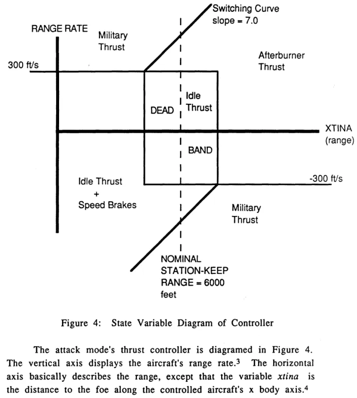
The attack mode's thrust controller is diagramed in Figure 4. The vertical axis displays the aircraft's range rate.3 The horizontal axis basically describes the range, except that the variable xtina is the distance to the foe along the controlled aircraft's x body axis.4 This variable was selected instead of the range in order to prevent a component of the range perpendicular to the x body axis from

3 The range rate is the negative of the closure rate.

4 The x body axis is a body-fixed axis which points straight out the nose of the aircraft. Xtina is a distance along this axis.

introducing a control input to the engine. Figure 5 shows a graphic depiction of the range variable xtina.

Aircraft Flying 'm• • lodle Range \ \1 \; Xtina .

..

Figure 5: Diagram of the Variable Xtina

The graph in Figure 4 describes a state space defined by the two variables. The space is separated into five control regimes by two switching curves and a dead band. Each of the control areas define a state for which the controller will select a different throttle setting. As an example of how the controller works, take the case where the target is 3000 feet (along the attacker's x body axis) ahead of a chasing attacker and the attacker is closing fast (greater than 300 feet per second). Intuition tells us that the attacker would fly past the target unless some measures were taken to decelerate. Using the graph, an xtina range of 3000 feet lies to the left of the dead band. A range rate less than +300 feet per second places the aircraft in the left bottom regime denoting idle thrust with speed brakes. Thus, the controller has selected maximum deceleration. The plane will slow in order to prevent over-shooting the target. Physically, the controller makes intuitive sense.

Analytically, the controller creates a second order thrust

control loop. The output, however, has four discrete states. One way

18

of analyzing the stability is to plot the two state variables throughout a run. _{The desired output would be a curve spiraling toward the} center and remaining within the dead band. Due to the extreme nonlinearities inherent in the system, this result is never witnessed. The reason is that the output state variables do not come close to changing linearly with the input throttle setting. As an example, the input range variable xtina changes drastically if the difference in the heading of the two planes changes even slightly. The variable xtina does not always decrease as the acceleration of a pursuing plane is set to maximum. _{It also depends on the pursued plane's turn rate} and acceleration. Because of this, the controller should not be

thought of as a real-time high-speed loop set to stabilize the relative position of the pursued plane. Rather, the controller is a throttle selector which attempts to prevent a pursuer from overshooting its target, while still maintaining a thrust level which enables it to pull maximum g's when necessary.

3.3 Thrust Controller Comparisons

In order to create a controller with the prescribed operating qualities, a method of testing which did not include the use of classical theoretical methods of control system analysis5 _was

necessary. _{Because of the simulation environment, this method was} already provided. _{Instead of using the same AML pilot to fly against} each other and modifying the aircraft, the aircraft were kept

constant while modifying the pilots. The pilots where changed by providing different thrust control logics to each and flying them

against each other with symmetrical initial conditions. The thrust controller was optimized by modifying six

parameters which determine when to switch states from one regime to another. _{Each new controller was tested against an earlier one} with different parameters in an attempt to determine the best

5 _{This could not be done because the controller is used to select throttle}

settings as a reference, not as a high-speed feedback loop. The delay between the times each new maneuver is selected by the AML pilot is two seconds. The frequency of the input changes is so small that it does not help to apply

frequency response methods of analysis to the controller. The best and easiest way to test the controller is use trial and error by flying it in the simulation.

19

combination of controller gain variables. The six modifiable parameters are: the nominal station-keep range, the slope of the switching curve, the two horizontal limits of the dead band, and the two vertical limits of the dead band. Each of these lines is shown in Figure 4.

The combat effectiveness measures were used to evaluate the performance of each set of thrust controller parameters.

Experimentation over forty engagements for each set of controller parameters yielded an optimal value for each of the variables. The best nominal station-keep range was 6000 feet. The slope of the switching curves was 7 sec- 1_{. The dead band was 1000 feet wide on}

each side of the nominal range, and 300 feet per second above and below the zero range-rate value.

Once the attack mode was perfected, it was combined with the single-state feedback evasion mode and implemented in the AML pilot. This pilot was then used in both the attacker and the target aircraft for all of the tests and correlations in the rest of the study.

20

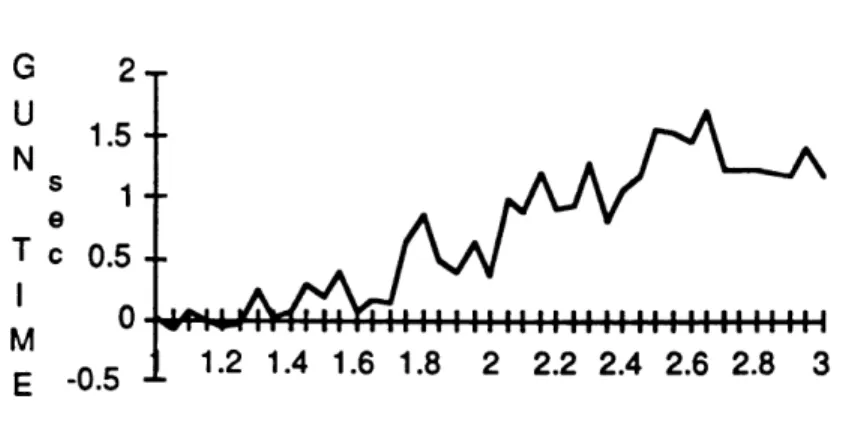
e. U 1.5-N s 1-e Tc 0.5.

Figure 6: Guns Time vs. G Multiplier

21

MO

In order to determine the results of the tests, the five performance parameters were compared with the three aircraft performance advancements both statistically and visually using various plots of the data. StatWorks was the software package used to perform the statistical analysis.

4.1 Correlation of Effectiveness Parameters with Load Factor Advantage

Figures 6, 7, and 8 display the Guns Time, Time on Offense (TOF) and the Time on Offense With Advantage (TOA) for the first sample runs. The vertical axis shows the effectiveness parameters averaged over fifty runs for each five percent increase in the

attacker's maximum g level. The independent variable, the g

multiplier, ranges from 1.0 (equal aircraft) to 3.0 (the attacker has 3 times the capability of the target). During the testing for the effect of the g ratio, the other two advantages, the thrust and speed brake multipliers, are held constant at 1.0 giving both planes the same thrust and maximum drag.

GLNS

T 0 I F 15 -M F 10 E Es Ne 5 NE 5 -5 -I 1.2 1.4 1.6 1.8 2 2.2 2.4 2.6 2.8 3 G ADVANTAGE

Figure 7: Offense Time vs. G Multiplier

In most of the graphs, the effectiveness of the attacker peaks at a g multiplier of 3.0. A g multiplier of 3.0 translates to a

maximum g loading of 27.0 g's because the F-18's maximum is 9.0. At this high value, the structural loading on the air frame is

unrealistic. Nevertheless, the study concludes that a higher maximum load level will assist.

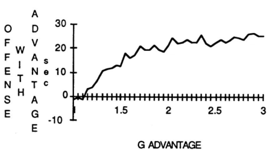
OFF W/ ADV A O D ov F W V 20-F As E Ne 10 T N TC H 0 S A E G E G ADVANTAGE

Figure 8: TOA vs. G Multiplier

22

As the g multiplier moves toward 3.0, all of the effectiveness parameters show that the attacker achieves higher and higher scores averaged over 50 fights.

OFFENSE TIME O0

I

- 1.5 IHII 2 2.5 lill lill 3AI

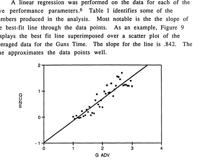
A linear regression was performed on the data for each of the

five performance parameters.6 _{Table 1 identifies some of the}

numbers produced in the analysis. Most notable is the the slope of the best-fit line through the data points. As an example, Figure 9 displays the best fit line superimposed over a scatter plot of the averaged data for the Guns Time. The slope for the line is .842. The line approximates the data points well.

0 1 2 3 4

G ADV

Figure 9: Scatter Plot of Guns Time (seconds) with Linear Regression

6 _{It was not necessary to perform a variance analysis so that the data could be} compared to the normal Fisher distributions. We know that any variance in the data can only be a result of the controlled independent variable. Every other possible input: initial conditions, weather, time, day, etc. that could change the dependent variable is held constant because we have run a computer simulation.

Effectiveness Slope of Best Standard Correlation Parameters Fit Line Deviation Coefficient (R)

(sec/mult) (sec' (unitless)

Guns Time .:842 .221 .918 All-Aspect Lock 1.349 .576 .818 Time Offense Time 8.388 1.529 .958 TOA 11.795 3.840 .881 (kills/mult) (kills) Number of Kills 12.146 4.456 .856

All of the correlation coefficients in the table are relatively high. The statistics show that all of the effectiveness parameters increase with increasing g load level, some to a greater extent than others. The slopes vary so much because it is more difficult for the attacker to obtain time in the weapons envelopes than it is to obtain time in the generalized offense envelopes. As a result, the vertical axis in effectiveness plots for the weapons envelopes have a smaller range than the Time on Offense (TOF) and the Time on Offense with Advantage (TOA).

The linear regression shows a strong correlation between the effectiveness parameters and the performance advantage. The positive slopes witnessed in each column of Table 1 indicate that with further increased g capability, the effectiveness measures continue to increase. _{Using the combat aircraft in this study, a} general law such as this one holds true only up to a g ratio of 3.0. Once the ratio of the maximum lift coefficient between the two planes exceeds 3.0, we begin to see different results.

24

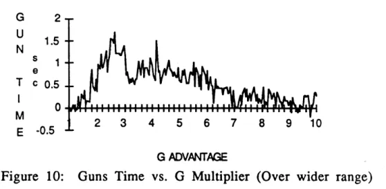
U 1.5 N s 1 e T c 0.5 0 M 0 G ADVANTAGE

Figure 10: Guns Time vs. G Multiplier (Over wider range) Figures 10, 11, and 12 show plots of the same effectiveness parameters displayed in Figures 6, 7, and 8 while the maximum load levels are permitted to vary from 1.0 (similar aircraft) to 10.0 (the attacker has ten times the capability of the target). The plots show that the effectiveness of the aircraft in combat continues to increase toward the maximum that we cited in Figures 6, 7, and 8, but then drops steadily. OFFENSE TIME T O 20 I F 15 M F S ₀ E Ee Nc 5

OS

0

Figure 11: Offense Time vs. G Multiplier (Over wider range)

25

GLUS

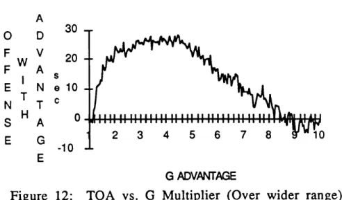
A 30 O D F WV 20-F A E N e 10 -N TT C S A E G 1- 0 2 3 4 5 6 7 8 10 E G ADVANTAGE

Figure 12: TOA vs. G Multiplier (Over wider range) This could be due to one of two possibilities: either the

attacker is unable to use the higher g levels because a g advantage greater than three times the foe's does not assist in the fight, or the present guidance logic is unable to guide the aircraft given such extensive normal acceleration capabilities. After studying several of the trajectories of the two aircraft throughout the higher g ratios, I find that the latter is true. The attacker tends to oscillate back and forth upon what looks to be the optimal trajectory to the opponent. This both wastes his energy and makes him take longer to gain a positional advantage or track the opponent. As a result, the target can turn back on him and in many situations, a reversal is

accomplished. Figures 10, 11, and 12 show that the data points generally head toward an effectiveness rating of zero as the g

multiplier increases beyond 3.0. The effectiveness parameters peak at a maximum load ratio around 3.0.

Overall, the data from the simulations permit a relatively good correlation to be made between the effectiveness parameters and g advantage. Over 2000 engagements were simulated in which only the g level was varied. Fifty sets of initial conditions were used. Combat effectiveness improved considerably with increases in airplane performance. The results indicate that it would be well worth it to devote time and effort into the research of autonomous

26

0.3 0.2 S e 0.1 c 0 -0.1 2 2.5 Figure 13: THRUST ADV

Guns Time vs. Thrust Advantage

Unlike the results from the previous correlation between the effectiveness in combat and the g advantage, these graphs seem to imply that increased thrust levels do not really assist the aircraft in combat.

27

vehicles whose performance limits are not hindered by the frailties of the human body.

4.2 Correlation of Effectiveness Parameters with Thrust Advantage

Similar tests were run modifying the attacker's thrust

capability. Two thousand engagements were simulated with fifty different initial conditions in which both the g multiplier and the speed brake multiplier were held constant at 1.0. Again, for each attacker configuration, the results from the fifty engagements were averaged for each of the five effectiveness parameters. Figures 13, 14, and 15 display this value for three of the parameters versus the increase in the thrust capability for the attacker.

ALL ASPECT

THRUST ADV

Figure 14: All-Aspect Missile Lock Time vs. Thrust Advantage

KILLS a U-

6-

Figure 15: Number of Kills in 50 Engagements vs. Thrust Advantage7 Again, a regression analysis was performed on the data. Figure 16 is an example of one of the best-fit lines attempting to relate the effectiveness of the attacker to its thrust advantage.

7 _{The effectiveness parameters are taken as the difference between the scores} of the attacker and the scores of the target. Therefore, negative values on the graphs of the parameters indicate that the target has attained a greater score than the attacker by the difference shown.

28 0.5 S e c -0.5

1.5

2

2.5

.. 0 2.2 2.4

Figure 16: Scatter Plot of Number of Kills with Linear Regression Examination of the scatter plot reveals large deviations from the least-squares line and a small slope. One would expect a

standard deviation which is large compared to the slope and a low correlation coefficient. _{The analysis was performed for each of the} five effectiveness parameters. Table 2 displays the results of the analysis.

Table 2: _{Linear Regression Analysis for Thrust Advantage} Effectiveness Parameters Guns Time All-Aspect Lock Time Offense Time TOA Number of Kills Slope of Best Fit Line (sec/mult) .089 -. 210 -2.233 -. 714 (kills/mult) .363 Standard Deviation (sec) .072 .286 .979 1.370 (kills) 2.470 Correlation Coefficient (R) (unitless) .499 .322 .726 .234 .068 29 o- -2--4 1.0 2.6 mu U *· U - · I I i 1.2 1.4 1.6 1.8 2 THRUST ADV

-4

100 80 C 60 o U n t 40 20 0 0 6 12 18 24 30 36 42 48 54 60 AFTERBURNER

Figure 17: Maximum Thrust Time Histogram

The horizontal axis is the amount of time (in seconds) that the afterburner throttle setting was used. The vertical axis shows the

30

The average correlation coefficient for Table 1 (g advantage) is .89 whereas that for Table 2 is only .37. The effectiveness values fluctuate rapidly without showing any sign of consistency. In general, due to the scattered nature of the plots and the poor

correlation coefficients in Table 2, we can conclude that a change in the thrust multiplier of the aircraft does little to affect the plane's performance in combat.

There are two possible reasons why the additional thrust did not assist the attacker in the fights: either the aircraft did not use its excess thrust, or, as simple as it may seem, extra tangential

acceleration is not needed in a game where normal acceleration is so important.

In investigating the former, thrust histograms were analyzed through 500 engagements. It was necessary to ensure that the enhanced configuration attacker was indeed using the excess thrust given to it. Figure 17 shows a histogram of the maximum thrust (afterburner) as it was used by the attacker in all of the five hundred engagements.

number of engagements for which the values were within the range indicated by the horizontal axis. Each engagement is sixty seconds long, thus there were a number of engagements (approximately 30 of 500) that used afterburner thrust close to 100 percent of the time. Most of the engagements seem to center around the 30 second to 36 second mark indicating that on the average, afterburner thrust was used over fifty percent of the time.

10C

E

24 0

Figure 18: _{3-D Military/Afterburner Thrust Histogram} Figure 18 displays the same afterburner histogram shown in Figure 17, but now it can be compared to the amount of time spent at military thrust throughout the 500 engagements. _{The time spent in} afterburner thrust is on the average much greater than that spent in military thrust. The greatest amount of time at which the throttle setting was military was only 24 of 60 seconds. From the two graphs we can conclude that the aircraft definitely used the thrust that it was given, especially since it selected afterburner thrust more times than not. The first explanation for a lack of correlation between effectiveness in combat and thrust advantage has been ruled out.

The second explanation, that normal acceleration is of much greater importance than extra tangential acceleration, seems to be more viable. If the excess thrust is used to accelerate the aircraft past the corner velocity, the maximum normal acceleration can no longer be obtained. Instead, the normal acceleration decreases with higher speed. As long as enough thrust is provided so that the

aircraft may remain near the corner velocity (to pull maximum g), extra thrust is of no consequence in most of the situations. This, in fact, seems to be the case. The baseline F-18 certainly has enough thrust to allow it to attain a sufficient turn rate to fight

competitively. Perhaps the F-18 is already over-powered and the excess can not be utilized. When the attacker was given the baseline configuration thrust, it did not use maximum thrust all of the time. Figure 19 will attest to this.

PERCENT OF 60 SECOND ENGAGEMENTS

30.64%

43% 59.90%

Figure 19: Average Time at Throttle Position (500 engagements) The graph displays the average amount of time that the throttle position was located in each region throughout 500

engagements of aircraft with equal thrust. Although afterburner thrust was selected 59.90 percent of the time, it was not used 100 percent of the time. For much of the average engagement, idle thrust was selected almost one-third of the 60 seconds. So, even when the attacker was given no thrust advantage, it did not use the maximum rating all the time.

32 SPEED BRAKES

O

33

_1_

When the aircraft does find itself in a bad situation, it will use the thrust in bursts in an attempt to get out of it. This is called disengagement. _{The study suggests that the pair of engines in the}

baseline aircraft were already sufficient to accelerate the plane out of any poor conditions. In the simulation, over many engagements with differing geometries, more thrust does not improve the

aircraft's combat performance.

In the history of aviation, we have seen a similar result. The A-4 Skyhawk is a combat aircraft which has proven itself to be a formidable foe. The interesting point here is that its engine is not a powerful one. It uses a single Pratt and Whitney J52-6 turbojet which has no afterburner. The engine carries a maximum thrust rating of 8,500 pounds8 _{whereas the baseline F-18 which flies}

against it carries a pair of General Electric F404-400 augmented turbofans rated at 16,000 pounds each.9 _{Until recently, the A-4 was}

still used as the U.S. Navy's main aggressor aircraft at Top Gun in NAS Miramar. Over many engagements, a greater thrust-to-weight ratio than already given to the F-18 did not assist except in a limited number of runs which usually involved one aircraft disengaging from the other.

4.3 Correlation of Effectiveness Parameters with Speed Brake Advantage

For the speed brake tests, the g multiplier and the thrust

multiplier were held constant at 1.0. The speed brake multiplier was varied through a range of 1.0 (similar aircraft) to 2.5 (attacker has 2.5 _{times the braking force of the target). Figures 20, 21, and 22} provide a graphical depiction of the plane's effectiveness in combat versus its brake advantage.

8 The E and J models carry this thrust rating. Models F, G, H, and K are rated at 9,300 pounds.

9 _{In addition, the loaded catapult weights of the A-4 and F-18 are 24,500 pounds} and 33,624 pounds respectively so the thrust-to-weight ratio is definitely in favor of the F-18.

0.15 0.1 0.05 0 -0.05 -0.1 Figure 20: 2.05

SPEED BRAKE ADV

Guns Time vs. Speed Brake Advantage

The figures seem to show, as was the result with the thrust advantage, that the enhanced capability for deceleration did not affect the aircraft's performance in the combat simulations. Three of the five effectiveness parameters are displayed.

OFF W/ ADV i V A s -1 Ne TC -2 A -3 G _-4

SPEED BRAKE ADV

Figure 21: TOA vs. Speed Brake Advantage

34

GUN TIME

-KILLS

iii. mull. liuuuul Ill liii

5- 4- 3- 2-1* -0 -1 2.55

SPEED BRAKE ADV

Figure 22: Number of Kills vs. Speed Brake Advantage

In addition, a statistical analysis provided similar results.

linear regression was performed for each of the five effectiveness parameters. Table 3 tabulates the results.

Table 3: Linear Regression Analysis for Speed Brake Advantage Effectiveness Parameters Guns Time All-Aspect Lock Time Offense Time TOA Number of Kills Slope of Best Fit Line (sec/mult) -. 016 -. 146 -. 182 .895 (kills/mult) .299 Standard Deviation (sec) .040 .141 .338 .830 (kills) 1.378 Correlation Coefficient (R) (unitless) .238 .535 .312 .549 .131

Figure 23 is a scatter plot showing the best fit to one of the effectiveness parameters.

2.05

35

III III .I II II III II I a I I

ý.f IV 1.5

- 4-K L L 2-L S 0--2 0 1 2 3 4 BRAKE ADV

Figure 23: Scatter Plot of Number of Kills with Linear Regression Speed brake advantage did not correlate well with the

effectiveness parameters. The correlation coefficients averaged only .353. The slopes of the best fit lines are highly variable, some

negative and some positive. The results show that, like the thrust advantage, the speed brake multiplier did not seem to assist the attacker in the simulated fights.

The reason this is true is easy to understand. When an aircraft is in combat, _{it is beneficial to keep both its potential and kinetic} energy high. This concept is inherent in the guidance logic of the AML which takes into account energy considerations. In addition, many military pilots have attested to the fact that it is important to maintain high speed so that the aircraft has the potential to

maneuver.

In keeping with its high energy strategy, the AML pilot used speed brakes only 4.04 percent of the time averaged over 500 engagements. Speed brakes were not used enough to make a difference in the fights. It is not worth the effort to provide high

speed aircraft with more efficient speed brakes.

36

• • IN

U Uri

I II

37

I

4.4 Correlation of Effectiveness Parameters with Combined Advantages

It has been shown that the speed brakes are not deployed a large enough percentage of the time to warrant their enhancement. However, afterburner thrust was used over fifty percent of the time. Yet, the measures of merit did not reflect an increase in combat effectiveness as the higher thrust advantage was provided to the attacker. _{A possible explanation was that the F-18 already has}

sufficient thrust to enable it to sustain a suitable airspeed to conduct high g maneuvers. _{However, when the baseline configuration was} given an increased maximum load level and consequently

experienced higher induced drag, the excess thrust might have been beneficial. _{In other words, the two advantages combined might have} made both of them worthwhile.

In order to test whether or not this hypothesis was true, the maximum load level multiplier was varied through a range of 1.0 (similar aircraft) to 3.0 (attacker has 3 times the capability) while the thrust multiplier was varied over the same range simultaneously. The two ranges of performance advantage represent a grid with the g advantage on one axis and the thrust advantage on the other. Each junction in the grid defines a configuration of the attacker for which 50 engagements were run. _{Again, the effectiveness parameters for} the 50 runs were averaged. _{Figure 24 provides a graphical depiction} of results.

Figure 24: 3-D Plot of Offense Time (seconds) vs. Thrust and G Advantages

The vertical axis of the plot is the offense time. The surface of the graph generally defines a sloping plane which is affected much more by the g advantage than the thrust advantage. However, as we move to the grid junctions where the thrust advantage is high, the average slope of the offense time with the g advantage is even steeper. This is even more visible in Figure 25, a graph similar to that of Figure 24, except that the effectiveness parameter is the number of kills.

Figure 25: 3-D plot of Number of Kills vs. Thrust and G Advantages

It seems as though the hypothesis was correct. For those aircraft capable of pulling the higher g levels and consequently suffering an increase in induced drag, the excess thrust was an

advantage. When the maximum load level multiplier was held at 1.0 (the same as the baseline configuration) the thrust increase was of no consequence. However, when the maximum load level was

increased, it was beneficial to the aircraft to increase thrust. This result forces a modification to the earlier conclusions about the benefits of excess thrust. It is true that, at equal g levels, extra thrust does not help. But as soon as one aircraft is provided a greater wing loading, it does help to increase the thrust so that the aircraft may take better advantage of its aerodynamic improvement. Therefore, the best attacker configuration consists of a combination

erformance advancements in both maximum thrust rating and mum g loading.

41

m

5. DEPENDENCE OF AIRCRAFT EFFECTIVENESS ON

ENGAGEMENT INITIAL CONDITIONS

Due to the random nature of the initial conditions for the

engagements, the question arises as to what kind of effect they may have on deciding the outcome of the fights. If one plane is placed directly behind the other in a weapons envelope, the one in the rear is going to become the instant victor before the fight even takes place. The outcome of the fights could be pre-determined by the engagement initial conditions. The objective here is to determine if the random initial conditions affected the scoring statistics.

In order to determine if the initial conditions affected the outcome of the engagements, plots were made of the effectiveness parameters versus the initial conditions over 500 engagements of

equal aircraft. It is easier to interpret the initial conditions if they are classified into the following three categories: initial specific

energy difference, initial heading difference, and the initial detection distance (range). All of the variables in the initial conditions list are represented in these three parameters by the following equations:

AEs = _{Es attacker - Es target}

Es attacker = ha + (Va2_{) / 2*g} Es target = ht + (Vt2) / 2*g

AH = Heading of Attacker - Heading of Target Range = [ (Xa - Xt)2 + (Ya-Yt)2 + (ha - ht)2 _{] 1/2}

where:

AEs is the initial specific energy difference ha is the attacker's altitude

ht is the target's altitude

V a is the initial speed of the attacker Vt is the initial speed of the target

g is the acceleration due to gravity (9.81 m/s2) AH is the initial heading difference

-1(

0 10 20 30

Init Range x 10^3

Figure 26: Guns Time (seconds) vs. Range (feet)

A statistical analysis of the relationship between Guns Time and the independent variable Range shows a low correlation coefficient of 0.017.

The graph in Figure 27 of the Offense Time versus Range shows a scattered circle. This effectiveness parameter, like the others,

shows no correlation with the range. The attacker's effectiveness had no relation to the initial distance to the target aircraft.

42

(Xt, Yt, ht) is the initial position of the target Range is the distance between combatants

when maneuvering was initiated

The three parameters describing the initial conditions of the engagements (AEs, AH, and Range) were plotted against the

effectiveness parameters to see if any relationship between them existed. Figure 26 is a plot of the Guns Time versus Range for 500 engagements.