Convex optimization methods for model reduction

(1)

Convex Optimization Methods for Model Reduction

by

Kin Cheong Sou

Submitted to the Department of Electrical Engineering and Computer

Science

in partial fulfillment of the requirements for the degree of

Doctor of Philosophy in Computer Science and Engineering

at the

MASSACHUSETTS INSTITUTE OF TECHNOLOGY

September 2008

@

Massachusetts Institute of Technology 2008. All rights reserved.

C)

I

1 -,

Author .

Department of 6Yectrical Engineering and Computer Science

August 29, 2008

Certified by

;I

/1/A

Certified by

Accepted by....

Luca Daniel

Associate Professor

Thesis Supervisor

Alexandre Megretski

Professor

Thesis Supervisor

...

'...

.

Terry P. Orlando

Chairman, Department Committee on Graduate Students

OFC TEH LOGY

S CT 2 2 2008

L IBR-AR, • • ES

(2)

(3)

Convex Optimization Methods for Model Reduction

by

Kin Cheong Sou

Submitted to the Department of Electrical Engineering and Computer Science on August 29, 2008, in partial fulfillment of the

requirements for the degree of

Doctor of Philosophy in Computer Science and Engineering

Abstract

Model reduction and convex optimization are prevalent in science and engineering appli-cations. In this thesis, convex optimization solution techniques to three different model reduction problems are studied.

Parameterized reduced order modeling is important for rapid design and optimization of systems containing parameter dependent reducible sub-circuits such as interconnects and RF inductors. The first part of the thesis presents a quasi-convex optimization approach to solve the parameterized model order reduction problem for linear time-invariant systems. Formulation of the model reduction problem as a quasi-convex program allows the flexi-bility to enforce constraints such as staflexi-bility and passivity in both non-parameterized and parameterized cases. Numerical results including the parameterized reduced modeling of a large RF inductor are given to demonstrate the practical value of the proposed algorithm.

A majority of nonlinear model reduction techniques can be regarded as a two step procedure as follows. First the state dimension is reduced through a projection, and then the vector field of the reduced state is approximated for improved computation efficiency. Neither of the above steps has been thoroughly studied. The second part of this thesis presents a solution to a particular problem in the second step above, namely, finding an upper bound of the system input/output error due to nonlinear vector field approximation. The system error upper bounding problem is formulated as an L2 gain upper bounding problem of some feedback interconnection, to which the small gain theorem can be applied. A numerical procedure based on integral quadratic constraint analysis and a theoretical statement based on L2 gain analysis are given to provide the solution to the error bounding problem. The numerical procedure is applied to analyze the vector field approximation quality of a transmission line with diodes.

The application of Volterra series to the reduced modeling of nonlinear systems is ham-pered by the rapidly increasing computation cost with respect to the degrees of the poly-nomials used. On the other hand, while it is less general than the Volterra series model, the Wiener-Hammerstein model has been shown to be useful for accurate and compact modeling of certain nonlinear sub-circuits such as power amplifiers. The third part of the thesis presents a convex optimization solution technique to the reduction/identification of the Wiener-Hammerstein system. The identification problem is formulated as a non-convex

(4)

quadratic program, which is solved by a semidefinite programming relaxation technique. It is demonstrated in the thesis that the formulation is robust with respect to noisy mea-surement, and the relaxation technique is oftentimes sufficient to provide good solutions. Simple examples are provided to demonstrate the use of the proposed identification algo-rithm.

Thesis Supervisor: Luca Daniel Title: Associate Professor

Thesis Supervisor: Alexandre Megretski Title: Professor

(5)

Acknowledgments

I would like to express my gratitude to my advisors Professor Luca Daniel and Professor Alexandre Megretski, who have shaped me into what I am like today. Luca has taught me a lot of electrical engineering aspects of my research as well as the attitude that I should take when I am faced with engineering challenges. In addition, Luca has also spent a lot of time helping me with my presentation skills, which I hope, will eventually match up to his standard. Alex, on the other hand, has profoundly influenced my way of conducting research. Through our discussions (and sometimes arguments), I finally started to learn the rope of conducting rigorous research. In addition, Alex has also shown to me that a lot of seemingly intractable problems can actually be solved, and I am oftentimes amazed by the creative solutions that he comes up with. In addition to my advisors, I would also like to thank Professor Munther Dahleh and Professor Jacob White for being my committee members and providing me with helpful suggestions. I would also like to acknowledge the support of the Interconnect Focus Center, one of the five research centers funded under the Focus Center Research Program, a Semiconductor Research Corporation and DARPA program.

Now it is time to mention my folks in the CP group. Sharing my office are Lei Zhang and Bo Kim. Lei is a good friend of mine and we hang out a lot. His personality changed the dynamics of the group - I witnessed the change of interactions between the people in the group before and after his arrival. Yan Li, who is Lei's wife, also happens to be my friend and we have had many enjoyable chats. Bo is a very charming lady who is also very nice to everybody that she comes across. I thank her for all those kind words and encouragements to the group members including me. Brad Bond is the buddy sitting initially behind me and then next door. We have had a lot of discussions of just about every topics, technical or non-technical. I also thank him for inviting me to his home in Tennessee during the wonderful Christmas in the year of 2006. Junghoon Lee also sits next door. He is one of the nicest guy I have ever met. Dmitry Vasilyev is also a good friend of mine. We have had lots of technical discussions, but we also have had lots of skiing trips together. Other members and former members of the group are also gratefully acknowledged. Tarek El Moselhy, Steve

(6)

Leibman, Laura Proctor, Homer Reid, Jaydeep Bardhan, Xin Hu, Shih-Hsien Kuo, Carlos Pinto Coelho, David Willis together made my stay in the CP group very enjoyable.

I thank my parents for their support and their constant updates of the home front. With-out their sacrifice I could not have achieved what I have achieved today. I have been away from home for too long, and I think it must be very hard on them because of the separation. I sincerely appreciate their patience for waiting for me to complete my long journey to obtain my PhD.

The last semester at MIT has been particularly eventful for me. It has been laden with difficulties and setbacks for me, one after another. The trace of this half year will forever live in my mind. Especially memorable in this difficult semester is Qin, who proved to me, finally there is something I really care about.

(7)

4 A Convex Relaxation Approach to the Identification of the Wiener-Hammerstein Model 1V Introduction ... Technical Background and Definitions . ... 4.2.1 System and model ... 4.2.2 Input/output system identification problem . . . 4.2.3 Feedback Wiener-Hammerstein system ... 4.2.4 Non-parametric identification of nonlinearity . . .... ... ...109 . . . . .110 . . . . .110 . . . . .113 4.1 4.2 7 )7 )9

..

.... .

..

.... .

(10)

4.3 Identification of Wiener-Hammerstein System - No Measurement Noise . . 114

4.3.1 System identification problem formulation . ... 115

4.3.2 Non-uniqueness of solutions and normalization . ... 121

4.3.3 Formulation of the system identification optimization problem . . .123

4.3.4 Properties of the system identification optimization problem . . . .125

4.4 Solving the Optimization Problem ... ... 127

4.4.1 Semidefinite programming relaxation . ... 127

4.4.2 Local search ... 131

4.4.3 Final optimizations ... 132

4.4.4 System identification algorithm summary ... 134

4.5 Identification of Wiener-Hammerstein System - with Measurement Noise . 134 4.5.1 System identification problem formulation . ... 135

4.5.2 Formulation of the system identification optimization problem . . . 136

4.5.3 Reformulation of SDP relaxation. ... .. .. . . 139

4.5.4 Section summary ... 140

4.6 Identification of Wiener-Hammerstein System - with Feedback and Noise . 141 4.7 Complexity Analysis ... ... 144

4.8 Application Examples ... 144

4.8.1 Identification of randomly generated Wiener-Hammerstein system with feedback ... 144

4.8.2 Identification of a transmission line with diodes ... 145

4.8.3 Identification of an open loop operational amplifier ... 147

4.9 Conclusion ... ... 149

(11)

List of Figures

2-1 A one dimensional quasi-convex function which is not convex. All the sub-level sets of the function are (convex) intervals. However, the function values lie above the line segment (the dash line in the figure). ... 28

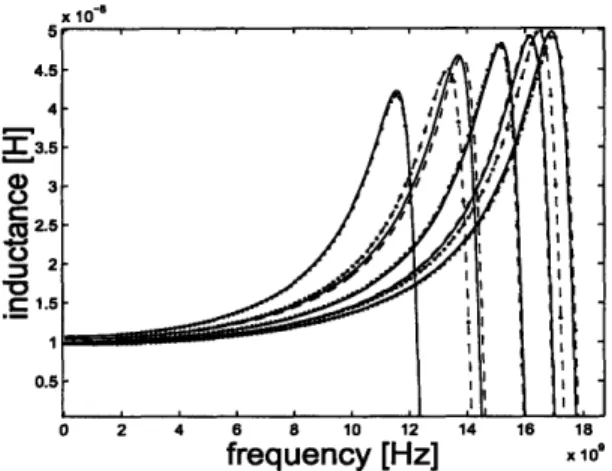
2-2 Magnitude of admittance of an RLC line. Solid line: full model. Solid with Stars: PRIMA 10th order ROM. ... 78 2-3 Magnitude of admittance of an RLC line. Solid line: full model. Solid with

Stars: QCO 10th order ROM ... 78

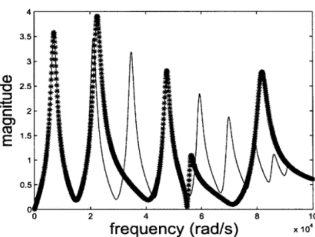
2-4 Inductance of RF inductor for different wire separations. Dash: full model. Dash-dot: moment matching 12th order. Solid: QCO 8th order. ... 79 2-5 Identification of RF inductor. Dash line: measurement. Solid line: QCO

10th order reduced model. Dash-dot line: 10th order reduced model using

methods from [14,55,57]... ... .. 80

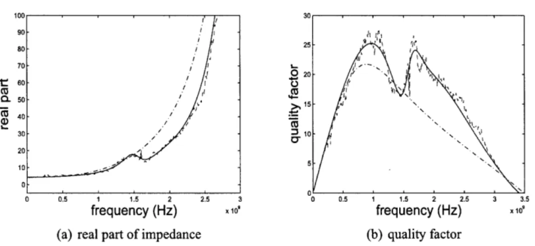
2-6 Magnitude of one of the port S-parameters for an industry provided ex-ample. Solid line: reduced model (order 20). Dash line: measured data (almost overlapping). ... 80 2-7 Quality factor of an RF inductor with substrate captured by layered Green's

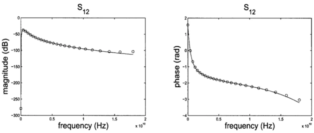
function. Full model is infinite order and QCO reduced model order is 6. . 81 2-8 S12 of the coupled inductors. Circle: Full model. Solid line: QCO reduced

m odel . . . 82

2-9 Quality factor of parameterized RF inductor with substrate. Cross: Full

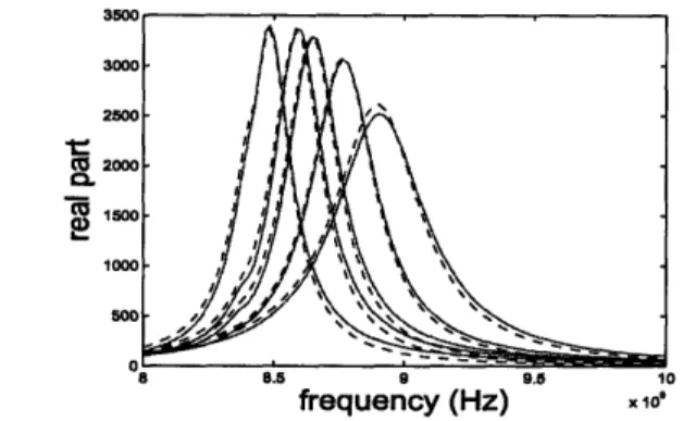
model from field solver. Solid line: QCO reduced model. ... 82 2-10 Real part of power distribution grid atD = 8.25 mm and W = 4, 8, 12, 14, 18

(12)

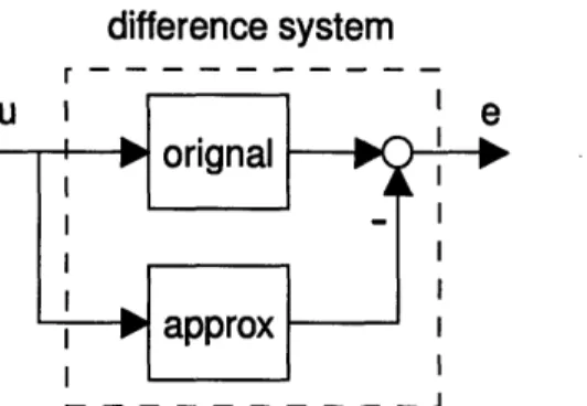
2-11 Real part of power distribution grid atD = 8.75 mm and W = 4, 8, 12, 14, 18 um. Dash: Full model. Solid: QCO reduced model. . ... 83 3-1 The difference system setup. The original system in eq. (3.1) and the

ap-proximated system in eq. (3.2) are driven by the same input u, and the difference between the corresponding outputs is taken to be the difference

system output denoted as e. The L2 gain (to be defined in Subsection 3.2.2) from u to e for the difference system is a reasonable metric for the

approx-imation quality between the systems in eq. (3.1) and eq. (3.2). . ... 86 3-2 Feedback interconnection of a nominal plant G and disturbance A. ... 91 3-3 Feedback interconnection of a nominal plant G and disturbance A with

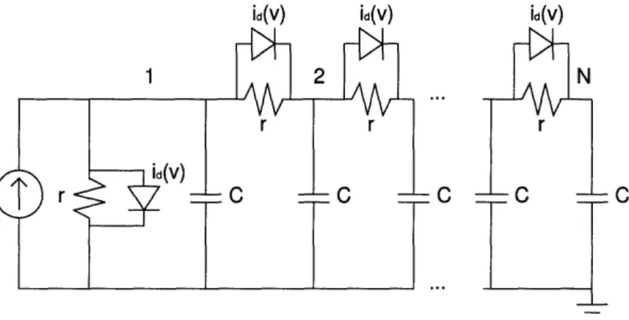
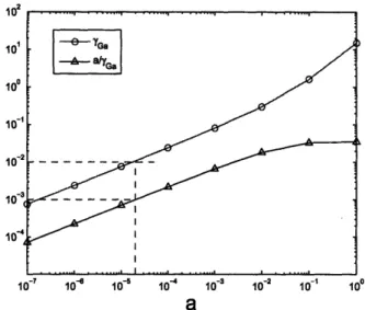
mu-tually cancelling parameters V/ and L. Ga is the original plant parame-terized by the scalar a. ... ... 96 3-4 A transmission line with diodes. . ... .... 104 3-5 Transmission line example. The upper line (circles) is the numerical upper

bound for the L2 gain of the difference system. The lower line (triangles) is the minimum allowable a such that 7ap < 1, and hence the small gain theorem still applies. For instance, if we want the system L2 gain error to be less than 10-2, then a should be at most 2 x 10- 5, corresponding to a maximum allowable vector field error Ya of about 10- 3. ... . . 105

4-1 The Wiener-Hammerstein system with feedback. S* denotes the unknown system. K = 0 corresponds to the Wiener-Hammerstein system without feedback. The output measurement y is assumed to be corrupted by some noisen* ... ... ... 111 4-2 The Wiener-Hammerstein model - G and H are FIR systems, and 4 is a

scalar memoryless nonlinearity. The last block is chosen to be H- 1 for computation reasons. ... ... 115

(13)

4-3 A feasibility problem to determine the impulse responses of the FIR sys-tems G and H. Here u and y are the given input and output measurements generated by the true (but unknown) system. The signals v and w are the outputs of G and H, respectively. v and w are chosen so that they define a function 0 satisfying sector bound constraint eq. (4.16). ... . . 117

4-4 Non-uniqueness of the optimal solutions without normalization. Given G* and H*, G and H characterize the family of FIR systems with the same in-put/output relationship. cl and c2 are positive because (G*, H*) and (G,H) are assumed/constrained to be positive-real. ... ... 122 4-5 Plot of A (s) in 200 (normalized) randomly generated directions. Note that

A (s) is not a convex function, but it is almost convex. . ... 126 4-6 Hyperbolic tangent test case. Histogram of the percentage of the second

largest singular value to the maximum singular value of the optimal SDP relaxation solution matrix X. The second largest singular values never ex-ceed 1.6% of the maximum singular values in the experiment. Data was collected from 100 randomly generated test cases. Nh = Ng = 4. ... 129 4-7 Saturated linearity test case. Histogram of the percentage of the second

largest singular value to the maximum singular value of the optimal SDP relaxation solution matrix X. X is practically a rank one matrix. Data was collected from 100 randomly generated test cases. Nh = Ng = 4. ... 130 4-8 Cubic nonlinearity test case. Histogram of the percentage of the second

largest singular value to the maximum singular value of the optimal SDP relaxation solution matrix X. For a lot of cases, the second largest singular values never exceed 5% of the maximum singular values in the experiment, but there are some cases when the SDP relaxation performs poorly. Data was collected from 100 randomly generated test cases. Nh = Ng = 4. .... 130

(14)

4-9 A feasibility problem to determine the impulse responses of the FIR sys-tems G and H. Here u and y are the given input and output measurement generated by the true (but unknown) system. The signals v and w are the outputs of G and H, respectively. The signal n is the noise corrupting the output measurement. In the feasibility problem, v, w and n are extra variables chosen so that, together with g and h, they define a function 0

satisfying sector bound constraint eq. (4.16). ... 135

4-10 The Wiener-Hammerstein model with feedback. ... 141 4-11 A feasibility problem to determine the impulse responses of G, H and

K * H. Here u and y are the given input and output measurement

gener-ated by the true (but unknown) system. The signals v and w are the input and output of the nonlinearity

4.

The signal n is the noise corrupting the output measurement. In the feasibility problem, v, w and n are extra vari-ables chosen so that, together with g, h and k * h, they define a function 0 satisfying sector bound constraint eq. (4.16). ... . . 142

4-12 Matching of output signals by the original (unknown) system and the iden-tified model. y[k] denotes the output by the original system (star). yi[k] denotes the output by the identified model (line). The plots of two output signals almost overlap. ... 145 4-13 Matching of the original nonlinearity (star) and the identified nonlinearity

(line) ... ... 145

4-14 A transmission line with diodes. . ... .... 146 4-15 Matching of the output time sequences of the original transmission line

sys-tem and the identified Wiener-Hammerstein model. Star: original syssys-tem. Solid: identified model ... 147 4-16 The inverse function of the identified nonlinearity 0. It looks like the

expo-nential V-A characteristic with an added linear function. ... 147 4-17 Block diagram of an operational amplifier. ... 148

(15)

4-18 First order model for the OP-AMP. The pole of the model is a nonlinear function of the outputy. The model fit in the feedback Wiener-Hammerstein structure discussed in this section. . ... ... 149 4-19 Matching of the output time sequence for a low frequency input test signal.

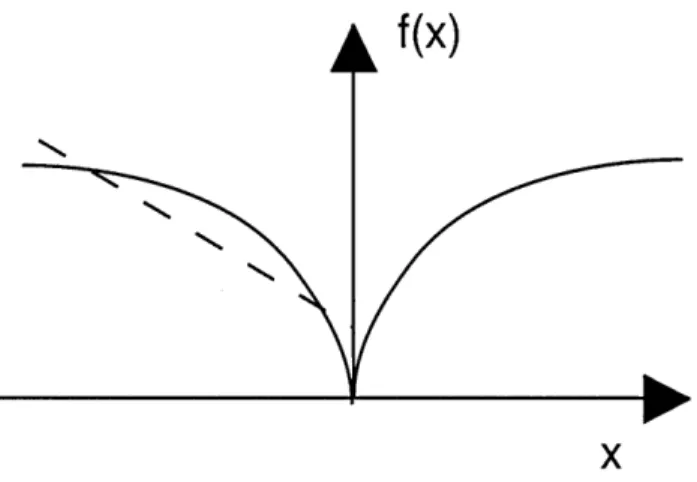
Dash: SPICE simulated output time sequence. Dots: subset of samples of the SPICE simulated output. Solid: identified model. ... 149 4-20 Matching of the output time sequence for a high frequency input test signal.

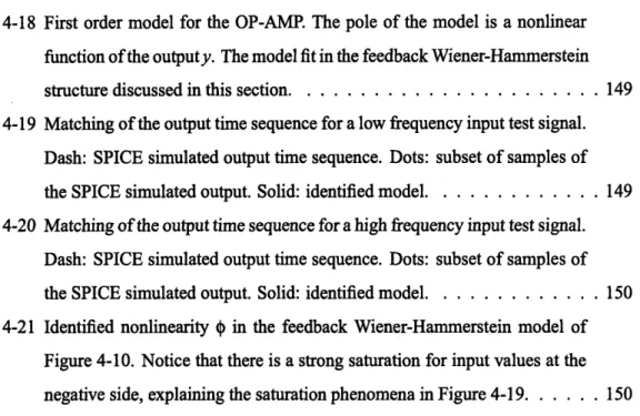
Dash: SPICE simulated output time sequence. Dots: subset of samples of the SPICE simulated output. Solid: identified model. ... 150 4-21 Identified nonlinearity ý in the feedback Wiener-Hammerstein model of

Figure 4-10. Notice that there is a strong saturation for input values at the negative side, explaining the saturation phenomena in Figure 4-19. ... 150

(16)

(17)

List of Tables

2.1 Reduction of RF inductor from field solver data using QCO and PRIMA . 77 4.1 The organization of Chapter 4 ... 109

(18)

(19)

Chapter 1 Introduction

1.1 Motivations

Model reduction is a widely accepted practice to facilitate system simulation and optimiza-tion. Different levels of success have been achieved depending on the specific model re-duction applications. Algorithms for model rere-duction for linear time-invariant (LTI) system

analysis have been successfully developed by many groups of researchers. For example,

balanced truncation (or truncated balanced realization) [1, 2, 3] and the optimal Hankel norm model reduction [4] are expensive model reduction algorithms (by the standard of the electronic design automation community) but they are very accurate and possess nice theoretical guarantees such as reduced model stability and error bound. On the other hand, moment matching (Krylov subspace methods) [5, 6, 7, 8] and proper orthogonal decompo-sition [9] are relatively inexpensive model reduction algorithms, but they do not in general offer much guarantee in terms of ready-to-use accuracy measures (e.g., X-, norm error bound) or reduced model properties such as stability. Only in some special cases can the stability of the reduced models be assumed [8]. In addition, compromises between the two groups exist approximating the first group using the operations allowed in the second group [10, 11, 12]. All the aforementioned algorithms construct reduced models by operat-ing on the state space representation (i.e., system matrices) of the full model and therefore are restricted to the model reduction problems of finite dimensional LTI systems. On the other hand, there are optimization/identification based model reduction algorithms which

(20)

directly find the coefficients of the reduced model without using the state space information of the full model. Rational transfer function fitting algorithms are well-known optimization based examples [13, 14]. In addition, rational transfer function fitting algorithms can en-force additional constraints such as stability and passivity. This will be shown in Chapter 2.

For the design and optimization of LTI systems, model reduction approaches have been less successful. One way to apply standard model reduction techniques to system design is to construct a reduced model for every full model ever considered by the design op-timizer. This path tends to be time-consuming because typically a large number of full models have to be considered and reduced. Another way to apply model reduction tech-niques to system design is to construct parameterized reduced models. Once such re-duced models have been constructed, the design optimization process can be greatly facil-itated. Due to their popularity in the non-parameterized case, the moment matching tech-niques have been extended to the parameterized reduction case by many previous attempts [15, 16, 17, 18, 19, 20, 21, 22, 23]. One significant drawback of the moment matching based parameterized model reduction techniques is that to increase the accuracy of the re-duced model, more moments need to be matched and this results in an increase in the order of the reduced model. The increase in order does not scales well with the number of param-eters. On the other hand, optimization based techniques such as rational transfer function fitting can be generalized to the parameterized case, constructing reduced models with or-ders independent of the number of parameters, even if an increase in accuracy is desired. However, the challenge with rational transfer function fitting is that with constraints such as stability, the reduced model construction process can be very time-consuming (because the optimization problems are not convex in general). Therefore, the development of a sta-ble reduced model generating rational transfer function fitting algorithm, which is efficient in both the model construction process and the simulation of the reduced models, would greatly benefit the design and optimization of LTI systems. The development of such an algorithm will be the main focus of Chapter 2.

The picture concerning the nonlinear model reduction problem is less clear simply be-cause "nonlinear" is a very general collective term for systems other than LTI. First attempt approaches for nonlinear model reduction include trajectory piecewise linear/polynomial

(21)

based methods [24, 25, 26, 27, 28, 29, 30] and Volterra series based projection methods [31, 32, 33, 34, 35, 36]. Trajectory based methods can be considered as two step proce-dures as follows: first the dimension of the system state is reduced by a projection, then an approximation is made to the reduced vector field for efficient simulation. Volterra series based projection methods, on the other hand, first approximate the vector field using poly-nomials and then reduce the approximated model using projection schemes. To make a tradeoff between reduced model accuracy and complexity (time required for model simula-tion), it would be necessary to understand how to quantify the error in the two steps. While in some cases the projection error (e.g., trajectory piecewise linear method with balanced truncation [27]) can be quantified, the error due to vector field approximation (i.e., the sec-ond step in trajectory based methods and the first step in Volterra series based projection methods) is not very well-known. An attempt to solve the vector field approximation error

estimation problem will be presented in Chapter 3.

Sometimes the only available information regarding the full model is its input and out-put measurements. On these occasions the projection based methods described above do not work. Instead, input/output based system identification techniques must be used to con-struct the reduced models. There is a very large body of input/output system identification techniques. See, for instance, [37, 38] for the descriptions of some of the techniques. The block diagram oriented identification technique based on the Wiener/Hammerstein/Wiener-Hammerstein structure is one of the most popular choices because of its simplicity, its abil-ity to model complicated nonlinear effects, and its applicabilabil-ity to model realistic devices such as power amplifiers and RF amplifiers [39, 40, 41]. Being a classical problem, the identification of the Wiener and Hammerstein systems and their combinations has been considered in a large number of references [42, 43, 44, 45, 46, 47, 48]. However, very few of the aforementioned references actually consider the Wiener-Hammerstein identification problem itself (i.e., two LTI systems sandwiching a memoryless nonlinearity) because of the "non-separability" issue (i.e., the cascading of three blocks with unknown coefficients makes the identification task much more difficult than the Wiener or Hammerstein setup with only two unknown blocks). The non-separability issue is oftentimes addressed by making certain assumptions on one of the blocks (e.g., assuming the nonlinearity to be of

(22)

certain forms such as polynomial), which might make the approaches restrictive in some cases. On the other hand, if no assumptions are made, the resulting identification decision problem would be very difficult (e.g., non-convex), and in general it is solved by a general purpose solver which might not be efficient. The purpose of the third part of the thesis is to investigate whether the identification decision problem possesses any special properties due to the underlying Wiener-Hammerstein structure, and whether these properties can be exploited in facilitating the optimization solution process. Chapter 4 presents in detail the relevant results.

1.2 Dissertation Outline

The following three chapters contain the contributions of this thesis. In Chapter 2 a quasi-convex optimization based parameterized model reduction algorithm for LTI systems will be presented. In Chapter 3 the problem of bounding the system error due to an approxima-tion to the nonlinear vector field will be considered. A convex optimizaapproxima-tion based numerical procedure and a theoretical statement will be given as solutions to the problem. In Chapter 4 a special case of the nonlinear model reduction problem, namely the Wiener-Hammerstein system identification problem, will be studied. A convex semidefinite programming based algorithm will be presented. Chapter 5 concludes the thesis.

(23)

Chapter 2 Model Order Reduction of

Parameterized Linear Time-Invariant

Systems via Quasi-Convex Optimization

Developing parameterized model order reduction (PMOR) algorithms would allow digital, mixed signal and RF analog designers to promptly instantiate field solver accurate small models for their parasitic dominated components (interconnect, RF inductors, MEM res-onators etc.). The existing PMOR techniques are based either on statistical performance analysis [49, 50, 51, 52, 10] or on moment matching [15, 16, 17, 18, 19, 20, 21, 22, 23].

Some non-parameterized model order reduction or identification techniques based on an optimization approach are present in literature. References [53] and [54] identify systems from sampled data by essentially solving the Yule-Walker equation derived from a linear least squares problem. However, these methods might not be satisfactory since the ob-jective of their minimization is not the norm of the difference between the original and reduced transfer functions, but rather the same quantity multiplied by the denominator of the reduced model. References [14] and [55] directly formulate the model reduction prob-lem as a rational fit minimizing the ~2 norm error, and therefore they solve a nonlinear least squares problem, which is not convex. To address the problem, those references pro-pose solving linear least squares iteratively, but it is not clear whether the procedure will converge, and whether they can handle additional constraints such as positive real

(24)

passiv-ity. In order to reduce positive real systems, the authors of [13] propose using the KYP Lemma/semidefinite programming relationship [56], and show that the reduction problem can be cast into a semidefinite program, if the poles of the reduced models are given a pri-ori. Reference [57] uses a different result derived from [58], to check positive realness. In that procedure, a set of scalar inequalities evaluated at some frequency points are checked. Reference [57] then suggests an iterative scheme that minimizes the H2 norm of the error system for the frequency points given in the previous iteration. However, this scheme does not necessarily generate optimal reduced models, since in order to do that, both the sys-tem model and the frequency points should be considered as decision variables. In short, the available methods lack one or more of the following desirable properties: rational fit, guaranteed stability and passivity, convexity, optimality or flexibility to impose constraints. In principle, the method proposed in this thesis is a rational approximation based model reduction framework, but with the following three distinctions:

* Instead of solving the model reduction directly, the proposed methodology solves a relaxation of it.

* The objective function to be minimized is not the H2 norm, but rather the 9-9, norm. As it turns out, the resultant optimization problem, as described in Section 2.2, is equivalent to a quasi-convex program, i.e., an optimization of a quasi-convex func-tion (all sub-level sets are convex sets) over a convex set. This property implies the following: 1) there exists a unique optimal solution to the problem; 2) the oftentimes efficient convex optimization solution techniques can be applied. Also, since the proposed method involves only a single optimization problem, it is near optimal with respect to the objective function used (i-. norm of error).

* In addition to the mentioned benefits, it will be demonstrated in the thesis that some commonly encountered constraints or additional objectives can be added to the pro-posed optimization setup without significantly increasing the complexity of the prob-lem. Among these features are guaranteeing stability, positive realness (passivity of

(25)

impedance systems), bounded realness (passivity of scatter parameter systems), qual-ity factor error minimalqual-ity. Also, the optimization setup can be modified to generate an optimal parameterized reduced model that is stable for the range of parameters of interest.

The rest of this chapter is organized as follows. Section 2.1 provides some technical background. Section 2.2 describes the proposed relaxation and explains why it is quasi-convex after a change of decision variables. Section 2.3 gives an overview of the setup of the proposed method and some details of it. Section 2.4 demonstrates how to modify the basic optimization setup to incorporate various desirable constraints. Section 2.5 focuses on the extension of the optimization setup to the case of parameterized model order reduction. In Section 2.6 more design oriented modifications will be discussed. As a special case, the RF inductor design algorithm will be given. In Section 2.7 the complexity of the proposed algorithm is analyzed. In Section 2.8 several applications examples are shown to evaluate the practical value of the proposed method in terms of accuracy and complexity.

2.1 Technical Background

2.1.1 Tustin transform and continuous-time model reduction

In order to work with (rational) transfer functions in a numerically reliable way, the fol-lowing standard procedure will be employed throughout the chapter: given a continuous-time (CT) system with transfer matrix He(s), first apply a Tustin transform (e.g., [59]) to

construct a discrete-time (DT) system H(z) := He(s)ls = X(z-1)/(z+1) (with X being a

pre-specified real number, to be discussed), then construct a reduced DT system Hi(z) using the proposed model reduction technique, and finally apply the inverse Tustin transform to

obtain the reduced CT system fic(s) := AI(z) I z=(j+s)/(X-s). The main benefit of the above

procedure is that the transfer function coefficients of the optimally reduced DT model will be bounded, thus making the numerical procedure more robust. In addition, except for the somewhat arbitrary choice of the parameter X in the Tustin transform, there is no ob-vious drawback for the model reduction procedure described above. Since the frequency

(26)

responses of the CT and DT systems are the frequency axis scaled versions of each other, there is an one-to-one correspondence between the (_9L norm) optimal reduced model in CT and DT with the same order. Consequently, model reduction settings for the rest of this chapter will be described in DT only.

The choice of the center frequency A in the Tustin transform is somewhat arbitrary. While it is true that extreme choices (e.g., picking X to be 1Hz, while the frequency range of interest is at 1GHz) can be harmful for the proposed model reduction framework, nu-merical experiments have shown that a broad choice of center frequencies would allow the proposed framework to work without suffering any CT/DT conversion problem. In fact, we have implemented, as part of the proposed model reduction algorithm, an auto-matic procedure that chooses the center frequency by minimizing the maximum slope of the magnitude of the frequency response, hence avoiding any possibly numerically harmful extreme situations.

2.1.2

1 norm of a stable transfer function

For a stable transfer function H(z) : C H C, the 1 norm is defined as

IIH(z)jll:=

sup

IH(eJW).

(2.1)

WE[0,21c)

The X5, norm for the multiple-input-multiple-output (MIMO) case with H(z) : C Cp'xn

(p 1,n > 1) is

IIH(z) 0 := sup I H(eJW) 12. (2.2)

co [0,2n)

The H1. norm can be thought of as the "amplification factor" of a system. In the context of model reduction, a reduced model HA(z) is regarded as a good approximation to the full

model H(z) if the X norm of the difference IH(z) - H^(z) is small.

2.1.3 Optimal XH2 norm model reduction problem

A reasonable model reduction problem formulation is the optimal H.- norm model reduc-tion problem: given a stable transfer funcreduc-tion H(z) (possibly of large or even infinite order)

(27)

and an integer m (as the order of the reduced model), construct a stable rational transfer function with real coefficients

II(z) = (z) := PmZm +Pm•1z' 1 + + PO pk E k E R, Vk

q(z) zm +q_m1zm- 1 ₊. . . + q 0

-such that order of AI(z) is less than or equal to m, and the error IJH(z) - AI(z) is

mini-mized:

minimize H(z) - P|

pq q zJ11.

(2.3) subject to deg(q) = m, deg(p) < m,

q(z) - 0, Vz E C, Iz I> 1 (stability).

Unfortunately, because of the stability constraint, program (2.3) is not a convex problem (see the next subsection for the definition). Up to now, no efficient algorithm for program (2.3) has been found.

2.1.4 Convex and quasi-convex optimization problems

This subsection will only describe the concepts necessary to the development of the thesis. For a more detailed description of the subject, consult, for example [60, 61].

A set C C Rn is said to be a convex set if

ax+

(1-a)yeC, VxE C,yE C, aE [0,1].

In other words, a set C is convex if it contains the line segment connecting any two points in the set.

A function f : RI -+ R is said to be convex if

f(axl + (1 - a)x2) < af(x) + (1 - a)f(x2), Vxl,x2 E "n, a E [0, 1].

In other words, a function f is convex if the function value at any point along any line segment is below the corresponding linear interpolation between the function values at the

(28)

two end points. In addition, a function f : R•n -R I is concave is -f is a convex function.

An optimization problem is said to be convex if it minimizes a convex objective func-tion (or maximizes a concave objective funcfunc-tion), and if the feasible set of the problem is convex. The nice property about a convex optimization problem is that any local opti-mum is also a global optiopti-mum. Convex optimization problems are oftentimes found to be efficiently solvable.

A relevant concept that will be explored in this chapter is the notion of a quasi-convex function. A function f : Rn -+ IR is quasi-convex if all its sub-level sets are convex sets. That is, the sets

{x E R"n f(x) < y} are convex, Vy E R.

The sub-level sets of a convex function are convex. Therefore, a convex function is auto-matically a quasi-convex function. However, the converse is not true. See Figure 2-1 for an illustration of a quasi-convex function which is not convex.

0. 1

Figure 2-1: A one dimensional quasi-convex function which is not convex. All the sub-level sets of the function are (convex) intervals. However, the function values lie above the line segment (the dash line in the figure).

A quasi-convex optimization problem is a minimization problem of a quasi-convex function over a convex set. Quasi-convex optimization problems are not much more diffi-cult to solve than convex problems. This is suggested by the fact that a local minimum of a quasi-convex problem is still a global minimum. In Sections 2.2 and 2.3 a specific class of

(29)

quasi-convex optimization problem will be identified, and an efficient algorithm to solve it will be detailed.

2.1.5 Relaxation of an optimization problem

While optimization provides a versatile framework for many model reduction decision problems, oftentimes the formulated optimization problems are difficult to solve (i.e., not convex). Formulating relaxations is a standard attempt to address the computation chal-lenge above. A relaxation of an optimization problem is a related optimization problem such that an optimal solution to the original problem is a feasible solution to the relaxation. A relaxation can be introduced if it is much easier to solve, and the optimal solution to the relaxation is useful in constructing a reasonably good feasible solution to the original prob-lem. However, note that such feasible solution might not be in general an optimal solution to the original problem. Typical ways for obtaining a relaxation include enlarging the fea-sible set and/or replacing the objective function with another (easier to optimize) function whose sub-level set contains the sub-level set of the original. It will be shown in Section 2.2 that the relaxation idea is useful in simplifying the proposed model reduction problem.

2.2 Relaxation Scheme Setup

This section describes the main theory of the proposed model reduction framework. The development of the framework is as follows: first a relaxation of (2.3) is proposed. Then a change of decision variables is introduced to the relaxation, and it can be shown that the relaxation is equivalent to a quasi-convex optimization problem, which happens to be readily solvable.

(30)

2.2.1 Relaxation of the X- norm optimization

Motivated by the optimal Hankel norm model reduction [62], the following relaxation of the optimal X1* norm model reduction was proposed in [63]:

minimize

H(z)

-

-(2.4) subjectto deg(q)=m, deg(p) m, deg(r) <m

q(z)

$

0, Vz e C,

Izl

> 1 (stability).

In program (2.4), an anti-stable rational part , where r is a real coefficient polynomial of degree less than m, is added to the setup of (2.3). Because of the associated additional decision variables (i.e., the coefficients of polynomial r), program (2.4) is a relaxation of (2.3). After solving program (2.4), a (suboptimal) stable reduced model can simply be obtained as Af(z) = P--). The following lemma, from [63], gives an error bound of the

relaxation.

Lemma 2.2.1. Let (p*,q*, r*) be the optimal solution ofprogram (2.4) with reduced order

m,

q*(z) q*(1/z) and

p*(z)

(z) := q*(z) be a stable reduced model, then

min { IH (z) -

I

(z) - D

I

}

< (m + 1) 7. (2.5) DER

Remark 2.2.2. By definition Y* is a lower bound of the error of the optimal H. norm

model reduction problem (2.3) and Lemma 2.2.1 states that the suboptimal reduced model provided by the proposed framework has an error upper bound (m + 1) times its error lower bound r*. In the lemma, I^(z) := * is the outcome of the solving program (2.4) orq* (z7

(31)

program (2.14), to be discussed in the next subsection. It should be noted that the scalar D in (2.5) can be incorporated into the reduced model fA, if HA is not a strictly proper transfer function. Therefore the reduced model should really be understood as A(z) + D* where

D* is chosen to be the optimizing D. In Section 2.3 procedure (2.26) will be discussed to

construct a reduced model that always picks the optimizing D. U

2.2.2 Change of decision variables in the relaxation scheme

The benefit of the relaxation (2.4) is not immediately obvious: program (2.4) still retains the non-convex stability constraint q(z) : 0, Vz e C,

Iz

I

> 1. More formally, it can be

stated that the set of the coefficients of the polynomials,

m "-pr

:

Np, E

)

Rm

x

Rm+l x Rm:

x

q(z) = znm + q-ml z m - 1 +... + qlz+ qo p(z) = #mZ + 1m-lz-m 1 +... + fiz +o (2.6) r(z) = ml-m - 1' +2m-2z n - 2 ₊ ... + satisfying q(z)

$

0, Vz E C: :

zi

1l

is not convex ifm > 2. As the first step to address the non-convexity difficulty, the following set of decision variables is proposed,

'b

:-

, b,{ I(

)

eR

m

_{x m+}

_x

a(z) = am(zm +z - m) +- a m- (zm-1 +z-m+l) + . ..+1

b(z) = bm(zm +z-m) +m-bm (zm- +z-m+l) + ...+ (2.7)

C(z) = 1('m(zm -z-m)+ . +1(Z-z-l)) satisfying a(z) > 0 Vz E C: Izi = 1.}

Note that the coefficient qm in eq. (2.6) is normalized to one because stability con-dition (i.e., E cannot have a pole at infinity) does not allow it to be zero. Likewise, the coefficient ao in eq. (2.7) is also normalized to one because positivity condition (i.e.,

(32)

in eq. (2.7), there is no normalization for am. In particular, it can be zero and the degree of a(z) can be strictly less than m. The following lemma defines an one-to-one correspon-dence between the sets qpr and bc, and hence suggesting that both sets can be used to

completely characterize the set of all reduced models in optimization problem (2.4).

Lemma 2.2.3. Define tm : Kmr - ambc as follows:

Given (4,p,i) E mpr, (8,b,) = Tm(qp,~) E Qabc is defined as follows: denote

m-1 )2

D:= I( + (k)2 ,then

(a,

b, are defined as the coefficients of the

trigono-k=0

metric polynomials

a(z) = Dq(z)q (z-1 )

b(z) = 2 [p(z)q (z-1) + q()r(z(z-') p (z-1) q(z) + q (z-1) r(z)] (2.8)

c(z) = 2ý[p(z)q (z- 1) + q(z)r (z-') - p (z-' ) q(z) - q (z-') r(z)].

* Given a,b, ) E 'am bc, (qpp) = m- 1 a,b, E pr is defined asfollows: let ri E {0,1,...,m} be the degree of a(z) in eq. (2.7), and let zk, k = 1,...,hM be the (maybe repeated) roots of the ordinary polynomial za(z) such that Izkl < 1. Then q is defined as the coefficients of the polynomial

q(z) := z' 11(z - zk). (2.9)

k=

m-1

-Denote D := 1 + ~ (k)2 , then p, r are uniquely defined by

k=O

D (p(z)q(z- ') + q(z)r(z-1)) = b(z) + jc(z). (2.10)

Then

1. The map tm is one-to-one with the inverse as tm-1

2. The map tm satisfies the following frequency response matching property:

H p(e) r(e-j) - b(eji) +jc(ejw)

H(ej m P) -(e~= a Ceo)< 2t. (2.11)

(33)

,-Proof of Lemma 2.2.3. The proof of the lemma is divided into three steps:

Step 1 shows that the definitions of the maps rm and "m-1 _{"make sense". That is,}

given (q, ', F) E f'pr, the operation of applying tm is valid, and it should be true that

(,b,) := Tm(q,p,F) E 0b c . Conversely, given (a,b,)E almbc, the operation of Tm- 1

is valid, and it should be true that (q, ,f) = Tm-_' _,b, _E m

pr

The first statement can be verified simply by applying the definition in eq. (2.8). For the second statement, suppose (a,b,) E bc is given. First show that the

opera-tion in eq. (2.9) is always valid, and q(z) thus obtained satisfies the condiopera-tion in eq. (2.6).

Let M^ be the degree of a(z), and define a(z) as

A(z) := za(z) = a,h (z_{? + 1) + a}2 _(Z2_&-_h- 1 _{+z) +...} ₊ .

The following properties of the roots of a(z) can be concluded: * Being an ordinary polynomial of degree 2m, a(z) has 2iA roots.

* Since ak = 0, the origin (i.e., 0 E C) cannot be a root of a(z). Therefore, zo E C is a root of ai(z) if and only if a(zo) = 0.

* Since a(z) has real coefficients and a(z) = a (z-'), the following two cases are true: ifzo E C \R is a root of (z), then so are zo', and Z, where is complex conjugate for z0 E C. On the other hand, ifz0 E R is a root of a(z), then so is I

* Since a(z) > 0,V I z = 1, there is no unit circle roots of a(z).

The four properties above imply that there are exactly MA stable roots and M^ anti-stable roots of A(z) as the "unit circle mirror images" of the former (e.g., 1 + 2j and 0.2 + 0.4j). Moreover, all roots with nonzero imaginary parts come in complex conjugate pairs. This concludes that the M^ roots described in eq. (2.9) can always be found, and q(z) defined in eq. (2.9) has real coefficients polynomial of degree m, and all roots of q(z) are stable (i.e.,

(34)

To conclude the proof of step 1, it remains to be shown that when

(

,b , E gfb is

given and q has been found by eq. (2.9), (p', ) E R2m+1 can be found as the coefficients of p(z) and r(z) using eq. (2.10). First recognize that eq. (2.10) defines a linear function

M4 : R2m+l H R2m+ 1 such that

M (,rF) = (, ). (2.12)

Then it is sufficient to prove that Mq is invertible. That is,

Ker (M) = 0. (2.13)

To show eq. (2.13), consider (p'*, ), corresponding to p*(z) and r* (z-') such that

p*(z)q (z- 1) - -q(z)r* (z-) .

The fact that q (z-') in the LHS has m stable roots and q(z) in the RHS has no anti-stable roots implies that r* (z- 1) should be m anti-stable roots. However, since the degree

of r* is strictly less than m, r* should be zero and p* should also be zero. This concludes that (p*, ) = 0 E R2m +1, showing that M4 is invertible and concluding step 1.

Step 2 shows that the map cm is one-to-one. For this purpose, it suffices to show the following: for every (q,p',i) E Q•pr, if q,, := -1 (Tm ( ,F,)), then ,,p =

(4, p, ,). First show that q= 4q. Let th E {0, 1,... , m} be the number of nonzero root of q(z),

then q(z) = z'm -5 (z -zk). Applying cm to (q , ,F) results in a a(z) with a known form.

k= 1

m m-1 -1

That is, a(z) = D [ (z -zk) (z- 1 -zk), with D = 1+ C (qk)2 .Then the ordinary

k=1 k=O

polynomial zma(z) in eq. (2.9) has exactly th stable roots (i.e., with magnitude less than one), and they are the roots of p(z) (i.e., zk for k = 1,2,... ,rM). Therefore, corresponding to q, the polynomial q(z) := zm -h IH (z-zk), is exactly the same as q(z), implying that

k=l

S=

4.

It remains to show that (, = (/, _{F). This is true because, for any}_4,_{the map}Mp q = q .s h w t a t t r m ai s t ý ) ( p qma p

4¢

(35)

defined in eq. (2.12) is invertible. Then,

=(M4

- 1

(M4 )

_=j

hence ,/,p) = (q, , p). This concludes step 2.

Finally, step 3 shows that the frequency matching condition in eq. (2.11) holds. Given

q ,c

,

E 0 'r, then simply by checking the definition in eq. (2.8), it can be verified that

(a,b, :=. m(q, p F) satisfies eq. (2.11).

Given, (, b4,)

e lC, because of the matching (up to the constant multiplicative

fac-tor D) of the numerafac-tor of eq. (2.11) by the definition in eq. (2.10), it suffices to show that q, as part of Tm-1' ,, ), satisfies the denominator matching of eq. (2.11) (i.e., a(z) = Dq(z)q(z-')). To show this, notice that for q(z) defined in eq. (2.9), Dz q(z)q (z- 1)

is an ordinary polynomial with exactly the same (stable and anti-stable) roots of za(z) be-cause of the "unit circle mirror image" property of the roots ofza(z) shown in step 1. That means that the coefficients of Dzq(z)q (z-') and Aza(z) can at worst be off by a constant multiplicative factor C. The coefficient of the monomial z of Aa(z) is one by the defini-tion in eq. (2.7). On the other hand, expressing q(z) as q(z) = zm + q,,_'Iz-' + ... + o0, it can be seen that the coefficient of the monomial

z

in Dz q(z)q (z-1_{) is also one, when}

D := 1+

:

(k)2 . Hence, the multiplicative factor C is one, and therefore q(z),

to-k=0

gether with a(z) satisfies the matching of a(z) = Dq(z)q(z- 1) in eq. (2.11). This concludes

step 3 and the proof of the lemma. M

Remark 2.2.4. Lemma 2.2.3 states that both sets mrp in eq. (2.6) and 2,c in eq. (2.7) can

completely characterize the relaxed model reduction problem in program (2.4). In addition, the stability constraint q(z) = 0, Vz E C : Iz > 1 in (2.6), which makes the feasible set of

(2.3) non-convex, can be replaced by the easier to handle (to be shown) positivity constraint

a(z) > 0, Vz E C : Iz

I

= 1, and this paves way to the discovery of efficient algorithms for

solving the relaxation problem. U

Remark 2.2.5. Since the evaluation of z in the positivity constraint in eq. (2.7) is restricted

to the unit circle only, for the model reduction problem in program (2.4), the evaluation of z can also be restricted to the unit circle because it is where the frequency response is

(36)

evaluated. Therefore, denoting z = e0co = cos(o) + jsin(o), program (2.4) is equivalent

to

minimize y

subject to jH(eji")(o) _{- b(co) - ji(o)l < ya(o), 0 < o < 2i,} _(2.14)

T(o) >0, 0 < o < 2n,

deg(i) < m, deg(b) < m, deg(O) < m,

with

ii(o) = 1 + aicos(oo) +..+ d~cos(mCo),

b(Co) = Lo + blcos(O) + ... + bmcos(mco) (2.15)

(o() = ~isin(o) ... +msin(mo)..

Because of the trigonometric terms, polynomials in eq. (2.15) (and in eq. (2.7)), are called

trigonometric polynomials of degree m. The following lemma justifies the change of vari-ables introduced by Lemma 2.2.3 in terms of possible computational efficiency gain. U

Lemma 2.2.6. Program (2.14) is quasi-convex (i.e., minimization of a quasi-convex

func-tion over a convex set). U

Proof of Lemma 2.2.6. First note that di(o) > 0, V o E [0, 2r) defines the intersection of infinitely many halfspaces (each defined by a particular Co E [0, 27r)) and therefore the feasi-ble set is convex. Secondly, consider a sub-level set of the objective function (for anyfixed

y). Since

Iz = maxRe(0z), Vz E C,

101=1 condition

|H(e`m)ii(o) - b(o) - jl(o)I < yi(Co), VCo e [0,27n)

is equivalent to

Re(0(H(eJ(o)a(c) -b (o) - j(co))) < ya(o), VCoe [0,21t), I10 = 1, (2.16)

which is the intersection of halfspaces parameterized by 0 and co. Therefore, the sub-level sets of the objective function of program (2.14) is convex and the quasi-convexity of the

(37)

Remark 2.2.7. Quasi-convex program (2.14) happens to be polynomially solvable. A

de-scription of how to solve the relaxation, as well as how this fits in the general picture of the proposed model reduction algorithm, will be discussed in the next section. Finally, it should be emphasized that not all quasi-convex programs are efficiently solvable. This is the case for the parameterized model reduction problem to be discussed in Section 2.5. U

2.3 Model Reduction Setup

This section deals with the solution procedure of the proposed model reduction framework.

A summary of the procedure is given as follows.

Algorithm 1: MOR

Input: H (z)

Output: H (z)

i. Solve program (2.14) using a cutting plane algorithm (details in Subsection 2.3.1) to obtain the relaxation solution (a, b, 0).

ii. Compute the denominator q(z) using spectral factorization eq. (2.9).

iii. Solve a convex optimization problem to obtain the numerator p(z). See Subsection

2.3.3.

iv. Synthesize a state space realization of the reduced model A/(z) = p(z)/q(z). See [59]

for details.

Step i. will be explained in Subsections 2.3.1 and 2.3.2. Step iii. will be explained in Subsection 2.3.3.

2.3.1 Cutting plane methods

Program (2.14) is a quasi-convex program with infinitely many constraints, and in general it can be solved by the cutting plane methods. This subsection will provide a general

(38)

description of the cutting plane methods, and their application to solving program (2.14) will be discussed in the subsequent parts of this chapter (Subsection 2.3.2 and Section 2.4). Note that the cutting plane method is a standard optimization solution technique for quasi-convex problems, and it is given here for completeness. The cutting plane method solves the following problem: find a point in a target set X (e.g., the sub-optimal level set of a minimization problem), or verify that X is empty. The basic algorithm description is as follows.

a. Initialize the algorithm by finding an initial bounding set P1 such that X C P1. b. At each step k, maintain a localization set Pk such that X C Pk.

c. Compute a query point xk E Pk. This is the current trial of the vector of the decision

variables. Check if xk E X.

d. If xk E X, then terminate the algorithm and return xk. Otherwise, return a "cut" (e.g.,

a hyperplane) such that all points in X must be in one side of the hyperplane (i.e., a halfspace). Denote the corresponding halfspace H.

e. Update the localization set to Pk+1 such that Pk n H C Pk+1,

f. IfVolume(Pk+l) < e, for some small e (which, for instance, is determined by the desired sub-optimality level), then assert X is empty, and terminate the algorithm. Otherwise, go back to step b.

The choice of the localization set Pk and the query point xk distinguishes one method from another. Reasonable choice of localization set/query point can be 1) a covering el-lipsoid/center of the ellipsoid or 2) covering polytope/analytic center of the polytope. The former choice results in the ellipsoid algorithm (see [64] or [65] for detailed reference), while the latter choice results in the analytic center cutting plane method (ACCPM) (see

[66] for reference). The finding of the initial bounding set P1 : X C P1 is problem

depen-dent, and it will be discussed in the next subsection, in the context of program (2.14). Step a. and step d. are the only steps in the cutting plane algorithm that are determined

(39)

(2.14), in Subsection 2.3.2 and Section 2.4, respectively. The subroutine implemented in step d. is typically referred to as an oracle. While the cutting plane algorithm is guaranteed to terminate in the number of iterations which scales polynomially to the problem size, the computation requirement of the oracle can range from light (e.g., the non-parameterized MOR case) to heavy (e.g., the parameterized MOR case).

Finally, it is noted that quasi-convex program (2.14) can also be solved as a semi-definite program (SDP) by interior point methods [67]. However, the discussion of this implementation will not be discussed in this thesis.

2.3.2 Solving the relaxation via the cutting plane method

In the context of solving the quasi-convex program (2.14) in Subsection 2.2.2, the de-scription of the cutting plane method introduced in Subsection 2.3.1 can be more specific: the decision variables x in Subsection 2.3.1 are the coefficients of the trigonometric poly-nomials a(co), b(co) and O(o). The target set X in Subsection 2.3.1 would be the set of trigonometric polynomial coefficients such that (2.14) is feasible (in particular, the stabil-ity constraint a&(o) > 0 is satisfied) and the objective value y can achieve its minimum (in practice, y is allowed to be within a few percents above the minimum).

A simple strategy to obtain an initial bounding set (i.e., PI in Subsection 2.3.1) is merely to assume it to be a "large enough" sphere. This is reasonable for most cases even though there is no real guarantee that it will work. However, for program (2.14), it is actually possible to find an initial bounding set which guarantees to contain the target set. The result is summarized in the following two statements.

Lemma 2.3.1. Let ak, k = 1,2,..., m be the coefficients of the trigonometric polynomial

t(co) in program (2.14), then the stability constraint a(o) > 0, VCo E [0, 2t) implies that

Iak <I 2, Vk= 1,2,...,m. I

Proof of Lemma 2.3.1. The stability constraint

(40)

implies that

27(o)

(1 +cos(kto))do >0, Vk= which (by the orthogonality of cosine) implies that

ak - - 2, Vk=l,2,...,m.

Similarly, eq. (2.17) also implies that

2(to) (1 - cos(km)) do > 0>, Vk= 1,2,...,m,

which in turns implies

ak•52, Vk=11,2,...,Im. (2.21)

Eq. (2.19) and (2.21) combined yields the desired result.

Lemma 2.3.2. Let ak, bk and jk be the trigonometric polynomial coefficients defined as

in eq. (2.15) in program (2.14). Let H(z) be any stable transfer function, and y be any nonnegative number Under the stability constraint 6i(o) > 0, Vo e [0, 27r), if it is true that

SB(o)+

j•(- _{o) -H(eJO)}

• y. (2.22)

Then

1.

IbkI

_ 2(2m+ 1) (IIH(z)

l.

+y),

2. Ikl

<

2(2m+

l)(llH(z)l I++y),

Vk=01,l,....)In

Vk= 1727...,IM.

Proof of Lemma 2.3.2. First prove the first statement. Eq. (2.22) implies that

(o)

-

Re [H(ei)] 5 y,

_(2.23)

because for any complex number x E C, IRe [x]

I

• Ixl. Eq. (2.23), together with the

trian-1,2,...,m, (2.18)

(2.19)

(2.20)

Convex optimization methods for model reduction

Convex Optimization Methods for Model Reduction

by

Kin Cheong Sou

Submitted to the Department of Electrical Engineering and Computer

Science

in partial fulfillment of the requirements for the degree of

Doctor of Philosophy in Computer Science and Engineering

at the

MASSACHUSETTS INSTITUTE OF TECHNOLOGY

September 2008

@

Massachusetts Institute of Technology 2008. All rights reserved.

C)

I

1

-,

Author .

Department of 6Yectrical Engineering and Computer Science

August 29, 2008

Certified by

;I

/1/A

Certified by

Accepted by....

Luca Daniel

Associate Professor

Thesis Supervisor

Alexandre Megretski

Professor

Thesis Supervisor

'...

Terry P. Orlando

Chairman, Department Committee on Graduate Students

ARCHIVES

OFC TEH LOGY

Convex Optimization Methods for Model Reduction

by

Kin Cheong Sou

Abstract

Acknowledgments

Contents

..

.... .

..

.... .

List of Figures

4.

List of Tables

Chapter 1

Introduction

1.1 Motivations

1.2 Dissertation Outline

Chapter 2

Model Order Reduction of

Parameterized Linear Time-Invariant

Systems via Quasi-Convex Optimization

2.1 Technical Background

2.1.1 Tustin transform and continuous-time model reduction

2.1.2

1

norm of a stable transfer function

IIH(z)jll:=

sup

IH(eJW).

(2.1)

2.1.3 Optimal XH2 norm model reduction problem

2.1.4 Convex and quasi-convex optimization problems

ax+

2.1.5 Relaxation of an optimization problem

2.2

Relaxation Scheme Setup

2.2.1

Relaxation of the X- norm optimization

minimize

H(z)

-

$

Izl

I

_{x m+}

_x

_=j