Magnetic refrigeration: recent developments and alternative configurations

HAL Id: hal-01315678

https://hal.archives-ouvertes.fr/hal-01315678

Submitted on 18 Mar 2017

HAL is a multi-disciplinary open access

archive for the deposit and dissemination of

sci-entific research documents, whether they are

pub-lished or not. The documents may come from

L’archive ouverte pluridisciplinaire HAL, est

destinée au dépôt et à la diffusion de documents

scientifiques de niveau recherche, publiés ou non,

émanant des établissements d’enseignement et de

Magnetic refrigeration: recent developments and

alternative configurations

Morgan Almanza, Afef Kedous-Lebouc, Jean-Paul Yonnet, Ulrich Legait,

Julien Roudaut

To cite this version:

Morgan Almanza, Afef Kedous-Lebouc, Jean-Paul Yonnet, Ulrich Legait, Julien Roudaut. Magnetic

refrigeration: recent developments and alternative configurations. European Physical Journal:

Ap-plied Physics, EDP Sciences, 2015, 71 (1), pp.10903. �10.1051/epjap/2015150065�. �hal-01315678�

Magnetic refrigeration

Recent developments and alternative configurations

Morgan Almanza, Afef Kedous-Lebouc, Jean-Paul Yonnet, Ulrich Legait and Julien Roudaut

CNRS, G2Elab, F-38000 Grenoble, France

Abstract – Magnetic refrigeration, based on magnetocaloric effect, is an upcoming environmentaly friendly technology with a high potential to improve energy efficiency and to reduce greenhouse gas emission. It is a multidisciplinary research theme and its real emergence requires, to overcome scientific and technical issues related to both material and system. This paper presents the state of the art in magnetic cooling, the main recent works achieved and discusses in more details the thermodynamic phenomenon according to the G2Elab experience in the field.

Keywords—Magnetic Refrigeration, magnetocaloric effect, magnetocaloric material, active magnetic regenerative cycle, modeling, experiment

1. INTRODUCTION

Refrigeration and air conditioning are essential to modern society to ensure health, security and to improve comfort. They contribute seriously to the global economy as they consume, according to the International Institute of Refrigeration (IIR), 15 percent of the worldwide electric energy, (20% in USA and 25% in Japan) with a 10 percent increase in demand each year and more in emerging countries.

Currently most of cold production is based on standard gas compression and expansion. This technology, dating back to the 19th, has the benefit of being mature. But today its energy consumption and pollution have to be reduced with firstly modification of our habit for rational use of the energy and secondly, development of more efficient and more eco-friendly technologies.

Besides active research in low global warming refrigerants (water, air, CO2, hydrocarbons, ammonia), the current works

target new solutions to produce cold. Magnetic refrigeration based on materials with magnetocaloric effect (MCE) is one candidate.

MCE is an intrinsic property of some materials which have a temperature change when they are magnetized in adiabatic condition. This effect is maximum at the magnetic phase transition temperature. MCE is used to make equivalent thermodynamic cycles to those done in cooling systems, playing with different thermodynamic variables. Magnetic refrigeration at room temperature could appear as a breakthrough cooling technology with a high efficiency potential, low pollution and an easy recycling thanks to the use of solid materials.

Even if MCE, the physical phenomenon used, has been known for more than a century, research in this area has really started 18 years ago following the discovery of new giant MCE

materials at room temperature by Gschneidner and Pecharsky ([1], Fig. 1) and the demonstration by Zimm et al of the feasibility of the magnetic refrigeration (Fig. 2).

Fig. 1. Magnetocaloric materials, reproduced from [2]

Fig. 2. Magnetic cooling device developed by Zimm et al [3]

Since, many major advances have been achieved at the fundamental and applicative scale in both materials and

systems. They progressively highlighted the complexity and the pluridisciplinarity of this research field which requires to analyze the entire physical phenomena involved as well as to investigate more and more accurate experiment and modeling studies. The different research activities can be gathered in the major following axes:

- Study of MCE and research of new materials with high magnetocaloric effect [4, 5]

- Study and modeling of thermodynamic cycles [6], - Design and realization of magnetic refrigeration

device with its magnetic source [7–9]

This paper presents the recent development done in the field and discusses the work led at the G2Elab in these last years in the frame of Interreg - Frimag and ANR - MagCool projects. It mainly focuses on thermodynamic aspects of the magnetic refrigeration.

2. MAGENTOCALORIC EFFECT

2.1. Thermodynamics

Thermodynamics gives appropriate tools to deal with MCE and magnetic refrigeration. At local thermodynamic equilibrium, the local variables chosen, magnetic field strength and temperature, depend on the considered position in the space. In the system studied, an elementary volume of magnetocaloric material (MCM), the first principle of thermodynamic is applied as shown in Eq. (1) with 𝑢 the internal volumic energy, −𝑀𝑑𝐵 the magnetic volumic work, 𝑄 the heat exchanged and 𝑞 the heat flux. The second principle is given at Eq. (2) in which 𝑠 is a state function associated to the volumic entropy and 𝑠_{𝑝𝑟𝑜𝑑𝑢𝑐𝑒𝑑} is a strictly positive function connected to the volumic entropy production. If the elementary volume is small enough to be considered in local thermodynamic equilibrium, Eq. (2) can be written in the form of Eq. (3). The partial derivative 𝑇 𝜕𝑠/𝜕𝑇|𝐻 defines the heat

capacity 𝑐𝐻 at constant field.

𝑑𝑢 = 𝛿𝑄 − 𝑀 𝑑𝐵 = −𝑑𝑖𝑣(𝛿𝑞 ) − 𝑀 𝑑𝐵 (1) 𝑑𝑠 = 𝑑𝑖𝑣 𝛿𝑞

𝑇 + 𝛿𝑠𝑝𝑟𝑜𝑑𝑢𝑐𝑒𝑑 (2) 𝑇𝑑𝑠 = 𝛿𝑄 + 𝑇𝛿𝑠𝑝𝑟𝑜𝑑𝑢𝑐𝑒𝑑 = 𝑐𝐻𝑑𝑇 + 𝑇_𝜕𝐻𝜕𝑠𝑑𝐻 (3)

Based on the 2nd principle, we define more rigorously the MCE, because it is important to distinguish the heat produced by losses directly linked to the irreversible effect of entropy production and the MCE with an entropy change due to the field variation which is a reversible process.

Therefore in adiabatic condition, the temperature change caused by MCE is computed through the resolution of an ordinary differential equation given by Eq. (4).

𝑑𝑇 𝑑𝐻= − 𝑇 𝑐𝐻 𝜕𝑠 𝜕𝐻+ 𝑇 𝑐𝐻 𝛿𝑠𝑝𝑟𝑜𝑑𝑢𝑐𝑒𝑑 𝑑𝐻 (4)

The Entropy production can be divided in two terms, one linked to the heat diffusion, hidden in 𝑑𝑖𝑣 𝛿𝑞 𝑇 and the

other linked to material entropy production 𝑠𝑝𝑟𝑜𝑑𝑢𝑐𝑒𝑑 . The last term, linked to material irreversibility (other than heat diffusion), will be neglected in the next part.

Therefore the characterization of MCE require the knowledge of three functions: 𝜕𝑠/𝜕𝐻(𝑇, 𝐻), 𝑐𝐻(𝑇, 𝐻) and the

magnetization 𝑀(𝑇, 𝐻). These information are obtained thanks to calorimetry, magnetometry and adiabatic temperature change measurements at different temperatures and fields [10]. Two mains issues occur. First the intrinsic properties determination needs to take into account mainly the effect of demagnetizing field in the test specimen. Second, these quantities must be interpolated to be numerically treated. And the functions found must ensure the thermodynamic consistency, i. e. they must keep energy conservation and avoid numerical entropy production artifact. Maxwell relations commonly used are based on this thermodynamic consistency.

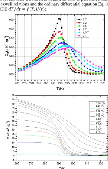
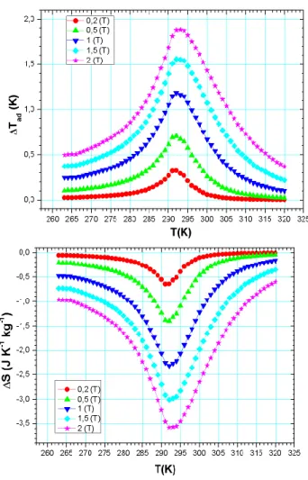
Fig. 3 gives the data curves obtained directly from measurement for a magnetocaloric manganite oxide and Fig. 4 the results after a numerical treatment. This is performed using Maxwell relations and the ordinary differential equation Eq. (4) (ODE 𝑑𝑇 𝑑𝑡= 𝑓(𝑇, 𝐻(𝑡)).

Fig. 3. Oxide Pr0.65𝑆𝑟0.35𝑀𝑛𝑂3 measured with a calorimeter and an extraction type magnetometer at CRISMAT laboratory (Caen – France)

Fig. 4. Properties deduced from Fig. 3 with the resolution of ODE and Maxwell relations

2.2. The basic thermodynamic cycle of the refrigeration With a MCE, an appropriate thermodynamic cycle gives us a cooling effect. Traditionally, the Brayton cycle is used (Fig. 5), it is based on four phases: 1- adiabatic magnetization, 2- iso-field heat exchange 𝑄𝑕𝑜𝑡 with the hot reservoir, 3- adiabatic

demagnetization and 4- iso-field heat exchange 𝑄𝑐𝑜𝑙𝑑 with the

cold reservoir. The temperature span between the hot and the cold reservoirs is written Δ𝑇𝑠𝑜𝑢𝑟𝑐𝑒.

The MCE materials performances are characterized by 3 main parameters: the adiabatic temperature change Δ𝑇𝑎𝑑𝑖𝑎, the

isotherm entropy change Δ𝑠_1𝑇 induced by an applied field variation (here taken as 1 T), represented on Fig. 5 by two black arrows and the Curie temperature 𝑇𝐶, where it achieves

the highest effects. In some systems, MCE operates only around a narrow temperature range thus the targeted MCM must have the larger Δ𝑠1𝑇 and Δ𝑇𝑎𝑑𝑖𝑎 at the appropriate 𝑇𝐶.

Whereas in others systems, MCE has to operate on large temperature range.

Performance of the thermodynamic cycles are defined by the exergy, itself given by the ratio of the cycle coefficient of performance COP, Eq. (4), to the COP of the Carnot cycle. Contrarily to the COP, it does not depend on Δ𝑇𝑠𝑜𝑢𝑟𝑐𝑒. For the

COP of the system, other works have to be added mainly pumping.

𝐶𝑂𝑃 = 𝑄𝑐𝑜𝑙𝑑 −𝑀𝑑𝐵

𝑐𝑦𝑐𝑙𝑒

(5) 2.3. Magnetocaloric Material (MCM)

MCM are classified by the order of the phase transition, i. e. the order of continuity of the free energy. The 2nd order phase transition materials present classical ferromagnetic/paramagnetic transition at 𝑇𝐶 while the first

order phase transition ones have a discontinuity on magnetization versus temperature or field. To go under thermodynamic description, additional transitions can take place in the first order materials as structural transition. This transition presents latent heat and often hysteresis because of metastable phenomena. The latent heat increases the entropy variation Δ𝑠1𝑇 as shown in Fig. 5 (area between dashed lines).

Fig. 5. Brayton Cycle for first order phase transition material. First order tansition is delimited by dashed lines

Fig. 6. |Δ𝑇_{𝑎𝑑 ,2𝑇}𝑚𝑎𝑥_{| as a function of |Δ𝑆}

2𝑇𝑚𝑎𝑥| for different compositions of MCM near room temperature. Diamonds represent experimental values, errors bars compositions effects and dots represent theoritical values. Figure taken from [11]

Fig. 7. Compound 𝐿𝑎𝐹𝑒𝐶𝑜𝑆𝑖: Curie temperature tuned by hydruration ratio [12]

MCM literature is extremely rich and the object here is not to make a partial list. We only mention the most promising of them in terms of refrigeration i. e. the LaFe or MnFe based compounds which are presented on Fig. 6. These materials have a very sharp transition which temperature is adjustable with compositions (Fig. 7). Intensive activities are currently underway to obtain these compounds at industrial scale [13]. 2.4. Comparaison with 𝐻𝐹𝐶 − 𝑅134𝑎 gas

The HFC R134a gas is commonly used as refrigerant and now regulations compel to progressively replace them with R1234yf, HC, CO2, ammoniac, etc. Comparison with

conventional gas compression system based on R134a is proposed in Table 1. An applied field of 1 T and a compression ratio of 4 are chosen as the operating point. They are realistic values. R134a gas has better performance than LaFeSiH in terms of Δ𝑠1𝑇 and Δ𝑇𝑎𝑑 𝑖𝑎 but others aspects need to be taken

into account as ability to exchange heat, working frequency, reversibility of the transformation… Mainly on these three aspects, MCM bring or could bring improvements: thermal conductivity is ten times higher, the process of magnetization and demagnetization can be fast and it is more reversible than gas compressors. Process means here, the way used to change the field or the pressure. For example, in the best cases, the efficiency of piston compressors is 70% [14].

Table 1. Gas data come from [15] where we assume to have the same amount of mass of fluide in evaporator and in condensor with respectively 16 Bar and 4 Bar. Refrigerant gas (R134a) Magnetocaloric (LaFeSiH) Δ𝑇𝑎𝑑𝑖𝑎 [𝐾] 45 3.5

Controled variable X 4 Bar - 16 Bar 0 T - 1 T

−Δ𝑆 [J. K−1_{. kg}−1_{] 400 10} −Δ𝑆 [mJ. cm−3_{] 240 71} 𝑐𝑋 [J. K−1. kg−1] 1300 1200 𝑐𝑋 [J. K−1. cm−3] 0.8 2.13 𝜆 [W. m−1_{. K}−1_{] 0.04 9} 3. MAGNETIC REFRIGERATION

To overcome the low value of Δ𝑇𝑎𝑑𝑖𝑎, a cascade of

thermodynamic cycles should be built as presented in Fig. 8. The temperature span between sources is then given by the

relation (6). The reservoirs constitute the heat storage elements, their temperatures are practically constant because their heat capacity is high and the average heat flow received is null. This cascade has an impact on the COP of the system. If the heat produced by losses is negligible compared to heat carried, the COP is given by the relation (7), where COPelem is the COP of

one stage and 𝑁 the number of stage, moreover the exergy stays constant. In practice, heat source appears because of not ideal thermodynamic transformation linked to material and irreversible cycle, but mainly because of not ideal device. Indeed device introduces heat, as viscous heat in the AMR system for example (cf 4). The heat must be evacuated to the hot reservoir and this leads to a faster decrease of the COP.

Thot − 𝑇𝑐𝑜𝑙𝑑 = Δ𝑇𝑠𝑜𝑢𝑟𝑐𝑒𝑁 (6)

𝐶𝑂𝑃 = 𝐶𝑂𝑃𝑒𝑙𝑒𝑚/𝑁 (7)

Fig. 8. Cascade of thermodynamic cycles for increasing temperature span between hot and cold reservoir comparison with one cycle

3.1. Heat exchange between cycles

The elementary cycle COP depends of the shape of the cycle itself. In order to analyze the influences of these exchanges, we adopt a simple model based on the concept of thermal switch, with 𝑘𝑜𝑛 the exchange coefficient when the

thermal conduction is wanted and 𝑘𝑜𝑓𝑓 when it is not.

Relations (7) and (8) come from the 1st and the 2nd principles of thermodynamics.

Fig. 9. Schematic of the model proposed with temperature 𝑇2 upper 𝑇1

Exergyelem .= 1

1 +𝑇𝑕 𝑜𝑡𝑆𝑝𝑟𝑜𝑑𝑢𝑐𝑒 𝐶𝑂𝑃𝑐𝑎𝑟𝑛𝑜𝑡

𝑄_{𝑐𝑜𝑙𝑑}

𝑆𝑝𝑟𝑜𝑑𝑢𝑐𝑒 = 𝛿𝑄 1 𝑇− 1 𝑇𝑟𝑒𝑠𝑒𝑟𝑣𝑜𝑖𝑟 𝐶𝑦𝑐𝑙𝑒 (9)

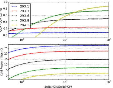
The analytic study on Brayton cycle shows that the exergy and the power increase when the ratio 𝑘𝑜𝑛/𝑘𝑜𝑓𝑓 and 𝑘𝑜𝑛

increase. Examples of these results are given in Fig. 10. We also show that 1st order materials, hence with latent heat, can significantly increase the exergy. Considering a cycle based on two isothermals and two adiabatic transforms, as similar study is presented in the paper [16]. Heat added by thermal switches has to be introduced for a more relevant study.

The AMR cycle explained in the part (3.3) has an equivalent 𝑘𝑜𝑛 of 8 kW. K−1. m−2 [17] whereas a mechanical

contact switch, without any pressure and common surfaces quality, gives a theoretically and experimental values of about 3 kW. K−1_{. m}−2 _{[18] and 1 kW. K}−1_{. m}−2 _{respectively.}

Fig. 10 Exergy and cold power evolution as a function of the ratio 𝑘𝑜𝑛. 𝑇𝑐𝑜𝑙𝑑 is 293 𝐾, the legend represents the temperatures of the hot reservoir with the characteristics of the MCM oxide Pr0.65𝑆𝑟0.35𝑀𝑛𝑂3 under 1 T (Δ𝑇𝑎𝑑𝑖𝑎= 1.2 K)

3.2. Magnetic source

The magnet volume is crucial for cost. With an ideal structure, meaning without leakage, we obtain the inequality (10) with: 𝑉𝑚𝑎𝑔 the volume of magnet and 𝑉𝑔 the volume

magnetized, 𝜇𝑟 the relative permeability, 𝐻𝑔 the field in the

MCM and 𝐽𝑚𝑎𝑔 the magnetic polarization. Therefore for a field

of 1 T in the MCM, four times larger volume is needed for a NdFeB magnet than for the magnetized area. Experimentally, we are around 7 [19]. Moreover a higher permeability MCM decreases the internal field.

𝑉𝑚𝑎𝑔 𝑉𝑔 > 4𝜇𝑟 𝜇0𝐻𝑔 𝐽𝑚 2 (10) With oxide and Δ𝑇𝑠𝑜𝑢𝑟𝑐𝑒 of 0.6 K, i. e. Δ𝑇𝑎𝑑𝑖𝑎/2 at 1 T, several

configurations can be considered: one stage with high field or multiple stages with low field. From numerical resolutions of equations (1) and (2), we show in Fig.11 that the increase in field allows the increase in exergy. The MMC makes the

Brayton cycles, with for the 1st stage the cold reservoir taken as cold heat storage and for the last stage the hot reservoir taken as hot heat storage.

3.3. AMR Cycle

AMR cycle (Active Magnetic Regenerative Refrigeration) is commonly used in magnetic refrigeration. In these systems, heat exchange is controlled by the fluid flowing alternatively through the material. With a parallel-plate regenerator and the use of symmetries, the study is reduced to the analysis of a half plate of fluid and MCM as shown in Fig. 12.

In Fig. 8, during the magnetized step the MCM exchanges heat with a single heat reservoir and when it reaches a temperature close to the temperature of the reservoir with which it exchanges, its magnetization is changed. Whereas in AMR cycle (Fig. 13), when the temperature is close to that of the reservoir, with which it exchanges, the MCM exchanges with a new reservoir. Its temperature is lower or higher, depending on the considered magnetization or demagnetization phase. Multiple reservoirs are introduced through the temperature gradient along the regenerator between temperature between 𝑇𝑕𝑜𝑡 and 𝑇𝑐𝑜𝑙𝑑. The heat exchange with

these reservoirs is controlled by the displacement of the fluid.

Fig. 11 Influence of stages cascade on exergy as a function of the applied field. Comparison with one stage at 1 T. The stages working point is Δ𝑇𝑟𝑒𝑠𝑒𝑟𝑣𝑜𝑖𝑟 = Δ𝑇𝑎𝑑𝑖𝑎/2 (which correspond to maximum power density) in the case of of Pr0.65𝑆𝑟0.35𝑀𝑛𝑂3.

Fig. 12.Scheme of the regenerator used in AMR cycle, complete representation on the left and the simplify one on the right. Blue arrows represent the velocity profil at different times

Fig. 13. Thermodynamic cycle in a TS diagram ; fluid is represented at F point and MCM at point M, these points correspond to Fig. 12

To operate a unique AMR cycle, materials with an effective MCE all over the temperature span of the regenerator are needed. This issue can be overcome by using the cascade structure shown in Fig. 8 where indeed the material works only around adiabatic temperature change Δ𝑇𝑎𝑑𝑖𝑎.

The AMR cycle can keep constant the temperature difference between the fluid and the material and therefore limits the undesirable entropy production due to heat exchange. In reality, this effect is limited as explained in the next paragraph. Entropy production rate due to heat flux is given by relation (11). Its minimization for a given heat exchange occurs when the temperature gradient is constant during the exchange. The demonstration is based on Lagrange multiplier and functional minimization.

𝜆 𝑔𝑟𝑎𝑑 𝑇

2

𝑇 𝑑𝑡 (11)

Concretely, fluid displacement must be limited to avoid unwished exchanges with the reservoirs sides. Indeed for a correct exchange, the temperature of the fluid must be respectively higher than 𝑇𝑕𝑜𝑡 or lower than 𝑇𝑐𝑜𝑙𝑑 at the hot or

the cold side. In the opposite case, the flow direction is reversed.

For the narrow 1st order phase transition material, different layers of MCM are used along the regenerator to maintain the MCE and therefore obtain a large temperature span working regenerator.

4. AMR SYSTEM

The AMR cycle was introduced and used by Barclay in 1982 [20]. It is now used in the majority of devices developed. The alternative heat exchange along the regenerator and the moving fluid amplifies the temperature span as indicated in section (3.3).

Several experimental and modeling approaches are used to study the AMR cycle and also the behavior of MCM in the working conditions [7, 23]. Thereafter, we discuss these points

on the base of recent developments and results obtained at G2Elab.

4.1. Experimental analysis of AMR cycle 4.1.1. Experimental device

Our device called DEMC and shown in Fig. 1 is a based permanent magnet system. It allows to study the AMR cycle for small size regenerator compatible with a small quantity of material, prepared at a laboratory scale [23]. The regenerator is static whereas the magnet, a Halbach cylinder of 0.8 T, is moving. The regenerator is a parallelepiped volume of 20 × 20 × 50 mm built with a stack of MCM plates. Other forms are possible for the material. It is alternatively magnetized or demagnetized when it is inside or outside the magnet. Two reservoirs are placed at the ends of the regenerator. They allow the fluid (water) to be stored which is essential to realize the AMR cycle. The fluid is alternatively moved with the use of two pistons. The magnet is also driven by an electric linear actuator. The system works in a closed loop, therefore all the regenerator is considered to be in adiabatic and no loaded conditions. The design has been made thanks to tridimensional simulations with finite element method. The control allows an easy and accurate choice of the working conditions.

For a given regenerator, the DEMC allows to study the effects of the cycle parameters as the flow, the frequency, the fluid moved volume, etc. It allows also testing different geometry of plates (thickness of fluid and MCM), shapes (sphere, powder), compositions, etc. This experiment is also used to validate analytical and numerical model developed. For example, Fig. 15 shows how starting from room temperature, we produce a hot and a cold sources at the ends of the regenerator and how their temperature evolve over time.

Fig. 14 Experimental device DEMC, here with a plates regenerator and an example of magnetic and fluidic cycles [23].

Fig. 15. Amplification of temperature span between cold and hot reservoir. The regenerator is made of Gd plates of 1 mm, with porosity of 20% and

Tadia=1.45 °C.

4.1.2. Results and discussion

The AMR device has been used to compare different regenerators with the same geometry but different materials: Gadolinium considered as the reference material, an intermetallic compound of LaFeSiCo produced by Vaccumshmelze GmbH&CO and a manganite oxide Pr0.65Sr0.35MnO3 produced by CRISMAT laboratory in Caen.

The two last one have been realized with compacted powders [23]. The main regenerator’s properties are shown in Table 2. Because PrSrMnOwas only available at laboratory scale, the number of plates was reduced from 17 to 11. The spacing between plates, ensured by different methods, gives different exchange width 22 mm for Gd and 20 mm for LaFeSiCo and PrSrMnO.

Table 2. Characteristics of the tested regenerators

Properties/ Regnerator Gd LaFeSiCo PrSrMnO

Regenerator volume Vr (cm3₎ 24 21 14 Porosity ε (-) 0.2 0.21 0.19 Fluid/Solid exchange surface (m2) 0.035 0.032 0.02 Density ρ(T = Tc) (kg.m-3₎ 7900 7150 6500

Specific heat capacity cH

(T = Tc) (J.kg-1_.K-1₎ 250 700 580 Thermal conductivity λ (T = Tc) (W.m-1 .K-1) 10.6 6 1.9 ∆Tadia (Bext=0.8T) (K) 1.45 1 0.5

For LaFeSiCo, two types of regenerators have been made: The 1st with a single material and the 2nd with 4 different layers having the following Curie temperatures 283, 288, 293 and 298 K.

The temperatures of the cold and the hot reservoir are measured for different flows of 0.5/1/2/3/4 ml.s-1, frequencies from 0.1 to 0.7 Hz and at an initial temperature (Ti) of 20°C +/- 1.5°C, except for one experimentation made at Ti = 25°C.

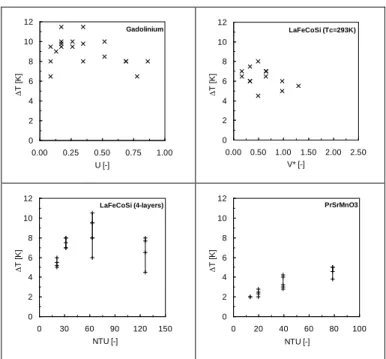
The T results obtained for the regenerators in different operating conditions are summarized in Fig. 16. To make an effective comparison, we introduce dimensionless quantities commonly used in heat and mass transfer:

- Volume factor V* : Represents the ratio of the fluid volume displaced during the flow period to the volume of the fluid contained in the regenerator (porosity dependence) ; - Utilization factor U : Represents the ratio of the fluid flow

thermal capacity to the material thermal capacity;

- Number of transfer units NTU: Represents the ratio of the thermal conductance to the fluid flow thermal capacity

Fig. 16. Comparative study of the performance of the 4 regenerators in Gd, LaFeSiCo and manganite oxide

Results give the optimal working conditions that allow reaching the maximum Δ𝑇 for the different regenerators. These values are 11.5, 10.5, 8 and 5°C for respectively Gd, LaFeCoSi multilayer, LaFeCoSi and Pr0.65Sr0.35MnO3. In spite of their

lower MCE and thermal conductivity, the PrSrMnO oxide exhibits interesting temperature span and could constitute a high potential material for magnetic refrigeration. A thinner oxide plate’s regenerator of 0.5 mm is also tested, to increase the heat transfer. A span of about 10°C is reached, which is equivalent to the span obtained with the 1 mm thick Gd regenerator.

4.2. AMR cycle Model

AMR cycle use a complex set of equations:

- equation (12), obtained from equation (2) applied on elementary volume, gives the thermal behavior of MCM; - equation (13) gives the thermal behavior of the fluid, with

𝑄𝑣𝑖𝑠𝑐 the viscous heating of the fluid;

- Navier-Stockes equation for incompressible flow; - Maxwell equations for magnetism

Entropy production has to be added to equations (12) and (13) to ensure strict energy conservation.

𝑐𝐻(𝑇, 𝐻) 𝑑𝑇 𝑑𝑡= ∇. 𝜆 𝑇, 𝐻 ∇𝑇 − 𝑇 𝜕𝑠 𝑇, 𝐻 𝜕𝐻 _𝑇 𝜕𝐻 𝜕𝑡 (12) Gadolinium 0 2 4 6 8 10 12 0.00 0.25 0.50 0.75 1.00 U [-] ∆ T [ K ] LaFeCoSi (Tc=293K) 0 2 4 6 8 10 12 0.00 0.50 1.00 1.50 2.00 2.50 V* [-] ∆ T [ K ] LaFeCoSi (4-layers) 0 2 4 6 8 10 12 0 30 60 90 120 150 NTU [-] ∆ T [ K ] PrSrMnO3 0 2 4 6 8 10 12 0 20 40 60 80 100 NTU [-] ∆ T [ K ]

𝑐 𝑑𝑇

𝑑𝑡+ v. ∇ T = ∇. 𝜆∇𝑇 + 𝑄𝑣𝑖𝑠𝑐 (13) The goal of modeling is to give tools to understand, predict and optimize the AMR cycles. Exact simulation of all this complex system, needs an important computation time and therefore it is not directly useful for optimization. Moreover, at this step of development, it can lead to irrelevant results because of persistence of uncertainties. It is the case of, boundaries conditions at the ends of the regenerator, the material characterization, the magnetic field homogeneity, the heat and mass flow, etc. In order to simplify the model, in the framework defined, assumptions at different levels are used. Without being exhaustive, we give an outline of the assumptions used in most of the literature models where plate’s regenerators are often considered:

– Based on symmetry and invariance consideration, the thermal and fluid simulations only focus on solving the problem for a half layer of water and MCM;

– In magnetism, the same symmetry and invariance principle is questionable especially for some regenerator shapes. However in the given framework, the demagnetizing factor coefficient is easy and sufficiently relevant to link the applied field to the internal field, mainly with respect to the criterion given by the ratio of accuracy/computation time given by 3D magnetic simulation;

– Fluid flow is not coupled to thermal and magnetic physics and thanks to a low Reynolds number, laminar flow is assumed. Moreover, the regenerator is supposed to be long enough to have an invariant flow profile along the regenerator.

Some shapes of regenerator could be far from the previous assumptions and in this case a more complex simulation has to be used to check the validity of assumptions made.

These assumptions are used for most of the models developed. Nowadays, mainly two complementary approaches emerge with more or less sophisticated materials models. 1D models are based on simplified convective exchange between the material and fluid. They often include the materials properties dependence on the field and the temperature [19, 25] but can use more simplified models [17]. The 2D models, solve the thermal equations in 2D, take into account the flow profile and therefore give a more accurate estimation of heat exchange between the fluid and the MCM.

4.2.1. 1D Models

It is a longitudinal 1D model which reduces the transverse dimension through integration over y in order to reduce the size of the system as shown in Fig. 12. 𝑇_𝑒 and 𝑇_𝑚 are fluid and MCM average temperatures given by the following mathematical expressions: 𝑇_𝑒𝑒_𝑒= _{𝑤𝑎𝑡𝑒𝑟} 𝑇𝑑𝑦 and 𝑇_𝑚𝑒_𝑚 =

𝑇𝑑𝑦

𝑚𝑐𝑚 .

Equation (14) gives the (simple) expressions used in 1D

model, with the viscous heating

𝑄𝑣𝑖𝑠𝑐 = 2𝜇 𝝏𝒗𝒙_𝝏𝒚 𝒚,𝒕 𝟐

on 𝒘𝒂𝒕𝒆𝒓 𝑑𝑦, 𝑉 the average fluid

velocity. All the variables related to the fluid and MCM have respectively a subscript e or m. 𝑒𝑚𝑐𝑚𝑑𝑇_𝑑𝑡𝑚 = 𝑄𝑖𝑛𝑡 + 𝑒𝑚𝜆𝑚𝜕 2_𝑇 𝑚 𝜕𝑥2 − 𝑒𝑚𝑇 𝜕𝑠 𝜕𝐻 𝜕𝐻 𝜕𝑡 𝑒𝑒𝑐𝑒 𝜕𝑇𝑒 𝜕𝑡 + 𝑉 𝜕𝑇𝑒 𝜕𝑥 = −𝑄𝑖𝑛𝑡 + 𝑒𝑒𝜆𝑒 𝜕2_𝑇 𝑒 𝜕𝑥2 + 𝑄𝑣𝑖𝑠𝑐 (14)

The 1D model simplifies the heat transverse exchange 𝑄𝑖𝑛𝑡

through the exchange coefficient 𝑕. 𝑄𝑖𝑛𝑡 = −𝜆𝑚

𝜕𝑇𝑚

𝜕𝑦 _𝑖𝑛𝑡 = 𝜆𝑒 𝜕𝑇𝑒

𝜕𝑦 _𝑖𝑛𝑡 = 𝑕 (𝑇𝑚− 𝑇𝑒) (15) In paper [19], a 1D numerical dynamic model has been implemented. The finite difference methods solve equations with an implicit method, chosen for an unconditional stability. The convergence of the numerical solution has been validated according to the discretization, initial condition and with comparison with obvious solution. Transient regenerator behavior is well shown and allows the four steps of the magnetic refrigeration cycle, to be clearly distinguished.

The 1D model can only solve the longitudinal heat exchange. All the transverse exchanges are described thanks to the exchange coefficient usually estimated from correlation table and which makes the approach open to criticism. In our case, fluid flow is alternating; we have a complex dependence with the geometry and the time. So the model reduction used is probably too strong to keep a sufficient accuracy. In [25], determination of h is experimentally corrected to fit the results of the AMR device.

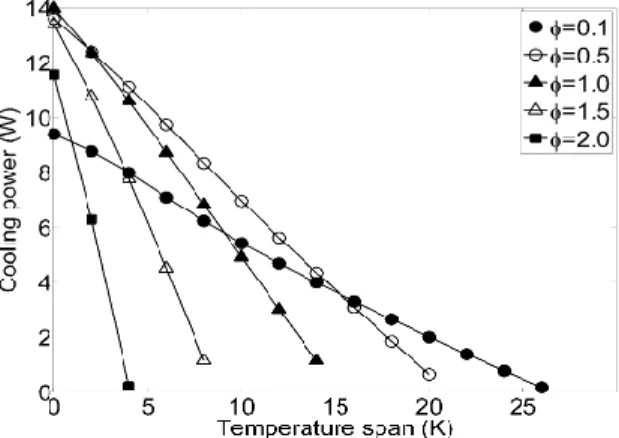
Fig. 17 and Fig. 18 show results from G2Elab experiment with Gd regenerator and from the 1D model developed. Results have been compared with those experimentally obtained with the DEMC. Qualitative agreement between simulations and measurements are observed. The curves have similar shapes and the maximal temperature spans are obtained near the same conditions. However, from a quantitative point of view, the model overestimates the performance of about 40%. Apart from intrinsic model limitation, these discrepancies can be explained by the regenerator imperfections and heat loss in the DEMC.

Fig. 17. Cold power as a function of T (NTU=0.5, with  is equal to U defined in the part 4.1.2), 1D model

Fig. 18.Comparaison : 1D model and experiment function of Tmax and flow rate

4.2.2. 2D model

The 2D model does not suffer from the approximation using the exchange coefficient h and therefore gives a more physical thermal description. In [17], a 2D model has been developed with FLUENT software considering a simple material model, with a constant Δ𝑇𝑎𝑑𝑖𝑎. This value is added or

subtracted to MCM temperature to simulate respectively a magnetization or demagnetization.

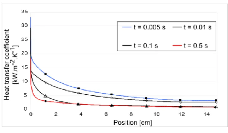
Fig. 19 shows the results obtained with the 2D model. As well as temperature evolution (Fig. 19.a), the model allows to estimate the coefficient of exchange h used in the 1D model (Fig. 19.b), the fluid flow velocity profile, the local viscous heating, etc. However, the required computation duration is 500 times higher than for 1D model (few seconds per period). This is a serious limiting factor for optimization. These types of models can be used in the last optimization steps, in order to validate the results of a 1D model. They also allow the optimal working point to be more accurately determined. It could be also used to compute the exchange coefficient h used in a 1D model.

a) 𝑇𝑕𝑜𝑡 and 𝑇𝑐𝑜𝑙𝑑 evolution with the number of cycles

b) Exchange coefficient along the regenerator at different times Fig. 19. Simulation result of AMR cycle with the 2D model

As for the 1D model, several simulations have been done with different thermal cycle parameters and compared to experiment (Fig. 20).

Fig. 20. Temperature span as a function of the fluid flow rate obtained with the Gd regenerator, comparison between Fluent 2D model and experiment. 5. CONCLUSIONS

Magnetic refrigeration development is based mainly on three axes of improvement: materials, thermal exchange and magnetic source.

Currently, the dominant MCM choices are the LaFe and MnFe based compounds. Fig. 6 shows that the theoretical values are much higher than those achieved today. This suggests considering that there is still a great potential of improvement, particularly as other compounds could be promising.

Historically, first magnetic cooling system was based on AMR cycle, and those of today tend to perpetuate this tradition. Progressive improvement in numerical simulation by both reducing computation time and increasing accuracy will allow, in the near future, the full potential of AMR technology to be evaluated.

Recently, new exchange concepts between cycles are investigated [26]. The concept of thermal switch proposes a unified approach which gives an easy access to the thermodynamics tools and offers to compare the different possibilities of exchange. New developments in thermal switches could be achieved exploring different methods: fluid, micro fluid, mechanical contact, thermal controlled interface,

2 3 4 5 6 7 8 9 10 11 12 13 0 2 4 6 8 Flow rate (ml/s) 𝚫T (K) Exp-f=0.7Hz Simu-f=0.7Hz Exp-f=0.35Hz Simu-f=0.35Hz

etc. However, this approach remains limited because it requires a large knowledge in different domains and in practice it is difficult to implement.

Magnetic source based in 𝑁𝑑𝐹𝑒𝐵 magnets are already well optimized [19]. However, for a reasonable mass of magnet in comparison to MCM mass (about 6 times) the magnetic field should be limited to about 1 Tesla.

6. ACKNOWLEDGEMENTS

The authors are grateful to the FEDER - European Regional Development Fund, the Switzerland confederation and the ANR French National Agency for Research for their financial support through the project FRIMAG (INTERREG IV A, France- Suisse n ° 2009/ 40) and MagCool (ANR STKE 2010-008).

7. REFERENCES

1. Pecharsky VK, Gschneidner, Jr. KA (1997) Giant Magnetocaloric Effect in Gd_{5}(Si_{2}Ge_{2}).

Phys Rev Lett 78:4494–4497. doi:

10.1103/PhysRevLett.78.4494

2. Pecharsky VK, Gschneidner Jr KA (1999) Magnetocaloric effect and magnetic refrigeration. J Magn Magn Mater 200:44–56. doi: 10.1016/S0304-8853(99)00397-2

3. Zimm C, Jastrab A, Sternberg A, Pecharsky V, Jr KG, Osborne M, Anderson I (1998) Description and Performance of a Near-Room Temperature Magnetic Refrigerator. In: Kittel P (ed) Adv. Cryog. Eng. Springer US, pp 1759–1766

4. GschneidnerJr KA, Pecharsky VK, Tsokol AO (2005) Recent developments in magnetocaloric materials. Rep Prog Phys 68:1479. doi: 10.1088/0034-4885/68/6/R04

5. Leitão JV, Brück E (2014) Magnetic and structural results on (Mn,Co)3(Si,P) and (Fe,Co)3(Si,P) alloys.

Results Phys 4:31–32. doi:

10.1016/j.rinp.2014.03.002

6. Nielsen KK, Tusek J, Engelbrecht K, Schopfer S, Kitanovski A, Bahl CRH, Smith A, Pryds N, Poredos A (2011) Review on numerical modeling of active magnetic regenerators for room temperature applications. Int J Refrig 34:603–616. doi: 10.1016/j.ijrefrig.2010.12.026

7. Yu B, Liu M, Egolf PW, Kitanovski A (2010) A review of magnetic refrigerator and heat pump prototypes built before the year 2010. Int J Refrig 33:1029–1060. doi: 10.1016/j.ijrefrig.2010.04.002 8. Bahl CRH, Engelbrecht K, Eriksen D, Lozano JA,

Bjørk R, Geyti J, Nielsen KK, Smith A, Pryds N

(2014) Development and experimental results from a 1 kW prototype AMR. Int J Refrig 37:78–83. doi: 10.1016/j.ijrefrig.2013.09.001

9. Sari O, Balli M (2014) From conventional to magnetic refrigerator technology. Int J Refrig 37:8–15. doi: 10.1016/j.ijrefrig.2013.09.027

10. Smith A, Bahl CRH, Bjørk R, Engelbrecht K, Nielsen KK, Pryds N (2012) Materials Challenges for High Performance Magnetocaloric Refrigeration Devices. Adv Energy Mater 2:1288–1318. doi: 10.1002/aenm.201200167

11. Sandeman KG (2012) Magnetocaloric materials: The search for new systems. Scr Mater 67:566–571. doi: 10.1016/j.scriptamat.2012.02.045

12. Rosca M (2010) Matériaux de type LaFe13-xSix à fort pouvoir magnétocalorique-Synthèse et optimisation de composés massifs et hypertrempés-Caractérisations fondamentales. Université de Grenoble

13. Alexandra Dubrez, Mayer C, Pierronet M, Vikner P (LaCe)(Fe,Mn,Si)13Hx Materials produced via gas atomization. Delft Days Magnetocalorics DMM 2013 14. Vrinat G (2014) Machines frigorifiques industrielles Introduction. Tech. Ing. Prod. Froid Mécanique base documentaire : TIB211DUO.:

15. Bejan A, Kraus AD (2003) Heat transfer handbook. J. Wiley, New York

16. Epstein RI, Malloy KJ (2009) Electrocaloric devices based on thin-film heat switches. J Appl Phys 106:064509. doi: 10.1063/1.3190559

17. Legait U (2011) Caractérisation et modélisation magnétothermique appliquée à la réfrigération magnétique. Université de Grenoble

18. Madhusudana CV (2013) Thermal contact conductance. Springer, New York

19. Roudaut J (2011) Modélisation et conception de systèmes de réfrigération magnétique autour de la température ambiante. Université de Grenoble 20. Barclay JA (1982) Theory of an active magnetic

regenerative refrigerator. NASA STIRecon Tech Rep N 83:34087.

21. Nielsen KK, Tusek J, Engelbrecht K, Schopfer S, Kitanovski A, Bahl CRH, Smith A, Pryds N, Poredos A (2011) Review on numerical modeling of active

magnetic regenerators for room temperature applications. Int J Refrig 34:603–616. doi: 10.1016/j.ijrefrig.2010.12.026

22. Yu B., Gao Q, Zhang B, Meng X., Chen Z (2003) Review on research of room temperature magnetic refrigeration. Int J Refrig 26:622–636. doi: 10.1016/S0140-7007(03)00048-3

23. Legait U, Guillou F, Kedous-Lebouc A, Hardy V, Almanza M (2014) An experimental comparison of four magnetocaloric regenerators using three different materials. Int J Refrig 37:147–155. doi: 10.1016/j.ijrefrig.2013.07.006

24. Legait U, Guillou F, Kedous-Lebouc A, Hardy V, Almanza M (2014) An experimental comparison of four magnetocaloric regenerators using three different materials. Int J Refrig 37:147–155. doi: 10.1016/j.ijrefrig.2013.07.006

25. Risser M, Vasile C, Muller C, Noume A (2013) Improvement and application of a numerical model for optimizing the design of magnetic refrigerators.

Int J Refrig 36:950–957. doi:

10.1016/j.ijrefrig.2012.10.012

26. Gu H, Qian X, Li X, Craven B, Zhu W, Cheng A, Yao SC, Zhang QM (2013) A chip scale electrocaloric effect based cooling device. Appl Phys Lett 102:122904. doi: 10.1063/1.4799283