HAL Id: hal-01418914
https://hal.archives-ouvertes.fr/hal-01418914
Submitted on 17 Dec 2016
HAL is a multi-disciplinary open access
archive for the deposit and dissemination of
sci-entific research documents, whether they are
pub-lished or not. The documents may come from
teaching and research institutions in France or
abroad, or from public or private research centers.
L’archive ouverte pluridisciplinaire HAL, est
destinée au dépôt et à la diffusion de documents
scientifiques de niveau recherche, publiés ou non,
émanant des établissements d’enseignement et de
recherche français ou étrangers, des laboratoires
publics ou privés.
What Else Is Decidable about Integer Arrays?
Peter Habermehl, Radu Iosif, Tomáš Vojnar
To cite this version:
Peter Habermehl, Radu Iosif, Tomáš Vojnar. What Else Is Decidable about Integer Arrays?.
Foun-dations of Software Science and Computational Structures, 11th International Conference, FOSSACS
2008, Mar 2008, Budapest, Hungary. �10.1007/978-3-540-78499-9_33�. �hal-01418914�
What else is decidable about integer arrays?
Peter Habermehl1, Radu Iosif2, and Tom´aˇs Vojnar3
1 LSV, ENS Cachan, CNRS, INRIA; 61 av. du Pr´esident Wilson, F-94230 Cachan, France,
e-mail:[email protected]
2 VERIMAG,CNRS, 2 av. de Vignate, F-38610 Gi`eres, France, e-mail:[email protected]
3 FIT BUT, Boˇzetˇechova 2, CZ-61266, Brno, Czech Republic, e-mail: [email protected]
Abstract. We introduce a new decidable logic for reasoning about infinite arrays of integers. The logic is in the∃∗∀∗first-order fragment and allows (1) Presburger
constraints on existentially quantified variables, (2) difference constraints as well as periodicity constraints on universally quantified indices, and (3) difference constraints on values. In particular, using our logic, one can express constraints on consecutive elements of arrays (e.g.∀i . 0 ≤ i < n → a[i + 1] = a[i] − 1) as well as periodic facts (e.g.∀i . i ≡20→ a[i] = 0). The decision procedure follows the
automata-theoretic approach: we translate formulae into a special class of B¨uchi counter automata such that any model of a formula corresponds to an accepting run of the automaton, and vice versa. The emptiness problem for this class of counter automata is shown to be decidable, as a consequence of earlier results on counter automata with a flat control structure and transitions based on difference constraints. We show interesting program properties expressible in our logic, and give an example of invariant verification for programs that handle integer arrays.
1
Introduction
Arrays are a fundamental data structure in computer science. They are used in all mod-ern imperative programming languages. To verify software which manipulates arrays, it is essential to have a sufficiently powerful logic, which can express meaningful program properties, arising as verification conditions within, e.g., inductive invariant checking, or verification of pre- and post-conditions. In order to have an automatic decision pro-cedure for the program verification problems, one needs a decidable logic.
In this paper, we develop a logic of arrays indexed by integer numbers, and having integers as values. To be as general as possible, and also to avoid having to deal explic-itly with expressions containing out-of-bounds array accesses, we interpret formulae over both-ways infinite arrays. Bounded arrays can then be conveniently expressed in the logic by restricting indices to be within given bounds.
Properties that are typically expressed about arrays in a program are (existentially quantified) boolean combinations of formulae of the form ∀i.G → V , where G is a guard expressioncontaining constraints over the universally quantified index variables i (which often range in between some existentially quantified bounds), and V is a value expressioncontaining constraints over array values. Based on examples, we identified two types of array properties which seem to appear quite often in programs: (1) proper-ties relating consecutive elements of an array, e.g.∀i . l1≤ i < l2→ a[i + 1] = a[i] − 1,
which states the fact that each value of a between two bounds l1and l2 is less than
its predecessor by one, (2) properties stating periodic facts, e.g.∀i . i ≡20→ a[i] = 0,
In the absence of specific syntactic restrictions, a logic with such an expressive power can be easily shown to be undecidable, as one can encode the histories of a 2-counter machine [13] as models of a formula over arrays. From this reduction, one can derive two restrictions leading to decidability. The first restriction forbids references to a[i] and a[i+ 1] in the same formula, which is considered in the work of Bradley, Manna, and Sipma [5]. The second restriction, considered in this paper, allows only array for-mulae∀i.G → V in which V does not contain disjunctions. We have chosen the second option, mainly to retain the possibility of relating consecutive arrays elements, i.e. a[i] and a[i + 1], which appears to be important for expressing properties of programs.
We introduce a new logic LIA (Logic on Integer Arrays) in the∃∗∀∗ first-order fragment. The logic LIA is essentially the set of existentially quantified boolean com-binations of (1) array formulae of the form∀i . ϕ(k, i) → ψ(k, i, a), where i is a set of index variables, a (resp.k) is a set of existentially quantified array (resp. array-bound) variables;ϕ is a formula on index variables with difference as well as periodicity con-straints on variables i wrt. the array-bounds k, andψ is a difference constraint on array terms, and (2) Presburger Arithmetic formulae on array-bound variables. In Appendix B, we give an example program showing the usefulness of this logic to express verifi-cation conditions.
In this paper, we prove the decidability of the logic LIA using the classical idea of the connection between logic and automata [18]: from a formulaϕ of the logic, we build an automaton Aϕ, such thatϕ is satisfiable if and only if Aϕis not empty. Decidability
of the logic follows from the decidability of the emptiness problem for the class of au-tomata that is deployed. To this end, we define a new class of counter auau-tomata, called FBCA (bi-infinite Flat B¨uchi Counter Automata). These are counter automata running to the infinity in both left and right directions, equipped with a B¨uchi acceptance condi-tion. For an arbitrary formulaϕ of LIA, we give the construction of an FBCA Aϕwhose
runs correspond to models ofϕ: the value of the counter xaat a given point i in an
exe-cution of Aϕcorresponds to the value of a[i] in a model of ϕ. We prove the decidability
of LIA by showing that the emptiness problem for FBCA is decidable by extending known results [6, 4] on flat counter automata with difference bound constraints. Related work. In the seminal paper [12], the read and write functions from/to arrays and their logical axioms were introduced. A decision procedure for the quantifier-free fragment of the theory of arrays was presented in [10]. Since then, various decidable logics on arrays have been considered—e.g., [17, 11, 9, 16, 1, 7]. These logics include working with various predicates (reasoning about sortedness, permutations, etc.) and in terms of various arithmetic (usually Presburger) constraints on array indices and/or val-ues of array entries. However, unlike our logic, most of these works consider quantifier free formulae. In these cases, nested array reads (like a[a[i]]) are allowed, which is not the case in our logic.
In [5], an interesting logic, within the∃∗∀∗fragment, is developed. Unlike our
deci-sion procedure based on automata theory, the decideci-sion procedure of [5] is based on the fact that the universal quantification can be replaced by a finite conjunction. The result is parameterised in the sense of allowing an arbitrary decision procedure to be used for the data stored in arrays. However, compared to our results, [5] does not allow modulo constraints (allowing to speak about periodicity in the array values), general difference constraints on universally quantified indices (only i− j ≤ 0 is allowed), nor reasoning
about array entries at a fixed distance (i.e. reasoning about a[i] and a[i + k] for a con-stant k and a universally quantified index i). The authors of [5] give also interesting undecidability results for extensions of their logic. For example, they show that relating adjacent array values (a[i] and a[i + 1]), or having nested reads, leads to undecidability. A restricted form of universal quantification within∃∗∀∗formulae is also allowed in
[2], where decidability is obtained based on a small model property. Unlike [5] and our work, [2] allows a hierarchy-restricted form of array nesting. However, similar to the restrictions presented above, neither modulo constraints on indices nor reasoning about array entries at a fixed distance are allowed. A similar restriction not allowing to express properties of consecutive elements of arrays then appears also in [3] where a quite general∃∗∀∗logic on multisets of elements with associated data values is considered. Remark. For space reasons, all proofs are deferred to Appendix D.
2
Counter Automata
Given a formulaϕ, we denote by FV (ϕ) the set of its free variables. If we denote a formula asϕ(x1, ..., xn), we assume FV (ϕ) ⊆ {x1, ..., xn}. For ϕ(x), we denote by ϕ[t/x]
the formula in which each occurrence of x is replaced by a term t. Given a formula ϕ, we denote by |= ϕ the fact that ϕ is logically valid, i.e. it holds in every structure corresponding to its signature. Byσ : Z → Z, σ(n) = n + 1, we denote the successor function on integers. In the following, we work with two sets of arithmetic formulae: difference bound matrices (DBM) and Presburger Arithmetic (PA).
A difference bound matrix (DBM) formula is a conjunction of inequalities of the form x−y ≤ c, x ≤ c, or x ≥ c, where c ∈ Z is a constant. If there is no constraint between xand y, we may explicitly write x− y ≤ ∞. In the following, Z∞denotes Z∪ {∞}. Let z= {z1, . . . , zn} be a designated set of variables, called parameters. A parametric DBM
formula is a conjunction of a DBM formula with atomic propositions of the forms x≤ f(z) or x ≥ f (z), where f is a linear combination of parameters, i.e. f = a0+ ∑ni=1aizi
for some ai∈ Z, 0 ≤ i ≤ n.
A Presburger arithmetic (PA) formula is a disjunction of conjunctions of either linear constraints of the form∑ni=1aixi+ b ≥ 0 or modulo constraints ∑ni=1aixi+ b ≡ c
mod d, where ai, b, c, d ∈ Z, c ≥ 0 and d > 0, are constants. It is well-known that every
formula of the arithmetic of integers with addition,Z, ≥, +, 0, 1- can be written in this form, by quantifier elimination [15]. Clearly, every DBM formula is also in PA.
A counter automaton is a tuple A= ,x, Q, −→-, where x is a finite set of counters, ranging over Z, Q a finite set of control states, and−→ the transition relation, given by rules q ϕ(x,x
.)
−−−−→ q., whereϕ is an arithmetic formula relating current values of counters
x to their future values x.. A configuration of a counter automaton A is a pair(q, ν) where q∈ Q is a control state, and ν : x → Z is a valuation of the counters in x. For a configuration c= (q, ν), we designate by val(c) = ν the valuation of the counters in c. A configuration(q., ν.) is an immediate successor of (q, ν) if and only if A has a
transition rule q ϕ(x,x
.)
−−−−→ q.such that|= ϕ(ν(x), ν.(x.)). A configuration c is a successor of another configuration c.if and only if there exists a sequence of configurations c= c0c1. . . cn= c.such that, for all 0≤ i < n, ci+1is an immediate successor of ci. Given
c0c1. . . cnwith c0= (q, ν), cn= (q., ν.) for some valuations ν, ν.: x→ Z, and ci+1is an
immediate successor of ci, for all 0≤ i < n.
Let S be a set. A bi-infinite sequence of S is a functionβ : Z → S.4We denote by ωSωthe set of all bi-infinite sequences over S. A bi-infinite B¨uchi counter automaton is
a tuple A= ,x, Q, L, R, −→-, where x is a finite set of counters, Q is a finite set of control states, L, R ⊆ Q are the left-accepting and right-accepting states, and −→ is a transition relation, defined in the same way as for counter automata.
A run of a bi-infinite B¨uchi automaton A is a bi-infinite sequence of configurations . . . c−2c−1c0c1c2. . . such that, for all i ∈ Z, ci+1 is an immediate successor of ci. A
run r is left-accepting iff there exists a state q∈ L and an infinite decreasing sequence of integers. . . < i2< i1< 0 such that for all j ∈ N, we have r(ij) = (q, νj) for some
valuationsνj of the counters of A. Symmetrically, a run is right-accepting iff there
ex-ists a state q∈ R and an infinite increasing sequence of integers 0 < i0< i1< i2< . . .
such that for all j∈ N, we have r(ij) = (q, νj), for some valuations νj of the
coun-ters of A. A run is accepting iff it is both left- and right-accepting. The set of all accepting runs of A is denoted as
R
(A). If r ∈R
(A) is a run of A, we define by val(r) = . . . val(r(−1))val(r(0))val(r(1)) . . . the bi-infinite sequence of valuations in r, andV
(A) = {val(r) | r ∈R
(A)}.Lemma 1. For any FBCA A, we have r∈
R
(A) if and only if r ◦ σ ∈R
(A).A control path in a counter automaton A is a finite sequence q0q1. . . qnof control
states such that, for all 0≤ i < n, there exists a transition rule qi ϕi
−→ qi+1. A cycle is
a control path starting and ending in the same control state. An elementary cycle is a cycle in which each state, except the first one, appears only once. A counter automaton is said to be flat iff each control state belongs to at most one elementary cycle.
Decidability and Closure Properties of FBCA We consider in the following the class of bi-infinite B¨uchi counter automata which are flat, and whose elementary cycles are labelled with parametric DBM formulae. We call this class FBCA in the following. We prove that the emptiness problem for FBCA is decidable, using results of [4], and their extensions, that can be found in Appendix A.
Lemma 2. The emptiness problem is decidable for the class of FBCA.
The FBCA class is also effectively closed under the operations of union and inter-section. However, before proceeding, we need to elucidate the meaning of these opera-tions for counter automata. If z⊆ x is a subset of the counters in x, let ν↓zdenote the
re-striction ofν to the domain z. For some subset z ⊂ x of the counters of A, and s ∈
V
(A), we define the restriction operator on sequences s↓z= . . . val(s(−1)) ↓zval(s(0)) ↓zval(s(1)) ↓z. . ., and
V
(A) ↓z= {s ↓z | s ∈V
(A)}. Symmetrically, for z ⊃ x, wede-fine the extension operator on sequences
V
(A) ↑z= {v ∈ω(z 4→ Z)ω| v ↓x∈V
(A)}.A class of counter automata is said to be closed under union and intersection if there exist operations5 and ⊗ such that, for any two FBCA Ai= ,xi, Qi, Li, Ri, →i-,
4In the early literature [14], a bi-infinite sequence is defined as the equivalence class of all
compositionsβ◦σn◦σ−mfor arbitrary n, m ∈ N. This is because a bi-infinite sequence remains
the same if shifted left or right. For simplicity reasons, here we formally distinguish the bi-infinite sequencesβ, β ◦ σn, andβ ◦ σ−n.
i= 1, 2, we have that
V
(A15 A2) =V
(A1) ↑x1∪x2 ∪V
(A2) ↑x1∪x2 andV
(A1⊗ A2) =V
(A1) ↑x1∪x2 ∩V
(A2) ↑x1∪x2, respectively. The class is said to be effectively closedunder union and intersection if these operators are effectively computable.
Proposition 1. Let A= ,x, Q, L, R, −→- be a FBCA. Let Ac= ,x, Q, Lc, Rc,−→- be the
FBCA such that (1) for all q∈ L and q.∈ Q, q.belongs to the same elementary cycle as q iff q.∈ Lc, (2) for all q∈ R and q.∈ Q, q.belongs to the same elementary cycle as q
iff q.∈ Rc. Then we have that
R
(A) =R
(Ac).Assuming w.l.o.g. that Q1∩ Q28= /0, the union is defined as A15 A2= ,x1∪ x2, Q1∪
Q2, L1∪ L2, R1∪ R2, →1∪ →2-. The product is defined as A1⊗ A2= ,x1∪ x2, Q1×
Q2, Lc1× Lc2, Rc1× Rc2, −→-, where −→ is as follows: (q1, q.1) ϕ1∧ ϕ2
−−−−→ (q2, q.2) iff q1 ϕ1
−→ q2is
a transition rule of A1and q.1 ϕ2
−→ q.2is a transition rule of A2. Here Lci and Rci, denote the
extended left-accepting and right-accepting sets of Ai, from Proposition 1, for i= 1, 2.
Lemma 3. The class of FBCA is effectively closed under union and intersection.
3
A Logic for Integer Arrays
In this section we define the Logic of Integer Arrays (LIA) that we use to specify properties of programs handling arrays of integers.
Syntax We consider three types of variables. The array-bound variables (k, l) appear within the so-called array-bound terms. These terms can be used to define the intervals of the indices, and also as static references inside arrays. The index (i, j) and array (a, b) variablesare used to build array terms. Fig. 1 shows the syntax of the logic LIA. We use the; symbol to denote the boolean value true. In the following, we will use f ≤ i ≤ g instead of f ≤ i ∧ i ≤ g, i < f instead of i ≤ f − 1, and i = f instead of f ≤ i ≤ f . Intuitively, our logic is the set of existentially quantified boolean combinations of:
1. Array formulae of the form∀i . ϕ(k, i) → ψ(k, i, a), where k is a set of array-bound variables, i is a set of index variables, a is a set of array variables,ϕ is an arithmetic formula on index variables, andψ is an arithmetic formula on array terms. In particular,ψ is a DBM formula, and ϕ is composed of atomic propositions of the form either f≤ i, i ≤ f , i − j ≤ n, i ≡st, where f is a linear combination of
array-bound variables, n∈ Z, and 0 ≤ t < s. Both k and a variables are free in the array formulae, but they can be existentially quantified at the top-most level. 2. PA formulae on array-bound variables.
Examples To accustom the reader with the logic, we consider several properties of interest that can be stated about arrays. For instance, a strictly increasing ordering of a up to a certain bound is defined as∃k ∀i . 0 ≤ i < k → a[i] − a[i + 1] ≤ −1. The fact that the first k elements of array a are below the first l elements of array b at distance 5 is defined as∃k, l ∀i, j . 0 ≤ i < k ∧ 0 ≤ j < l → a[i] − b[ j] ≤ −5. Equality of two arrays up to a certain bound can be expressed as∃n∀i . 0 ≤ i < n → a[i] = b[i]. The use of modulo constraints as guards for indices allows one to express periodic facts, e.g. ∀i, j . i ≡20 ∧ j ≡21→ a[i] ≤ a[ j], meaning that any value at some even position is
n, m, s,t . . . ∈ Z constants(0 ≤ t < s)
k, l, . . . ∈ BVar array-bound variables
i, j, . . . ∈ IVar index variables
a, b, . . . ∈ AVar array variables
B := n | k | B + B | B − B array-bound terms
I := i | I + n index terms
A := a[I] | a[B] array terms
G := B ≤ I | I ≤ B | I − I ≤ n | I ≡st| G ∨ G | G ∧ G guard expressions
V := A ≤ B | B ≤ A | A − A ≤ n | V ∧V value expressions
C := B ≤ n | B ≡st array-bound constraints
P := ; → V | G → V | ∀i . P array properties
U := P | C | ¬U | U ∨ U | U ∧ U universal formulae
F := P | ∃k . F | ∃a . F LIA formulae
Fig. 1. Syntax of the logic LIA
less than or equal to any value at some odd position in a. Appendix B shows that to prove the correctness of an array merging program, such properties are needed. Semantics The logic LIA is interpreted on both-ways infinite arrays. This allows to conveniently deal with out-of-bound reference situations quite common in programs handling arrays. One can prevent and/or check for out-of-bound references by introduc-ing explicit existentially quantified array-bound variables for array variables. Letϕ(k, a) be any formula of LIA. A valuation is a pair of partial functions5,ι, µ-, with ι : BVar ∪ IVar→ Z⊥, associating an integer value with every free integer variable, and µ : AVar→ ωZω
⊥, associating a bi-infinite sequence of integers with every array symbol a∈ a. The
valuationι is extended in the standard way to array-bound terms (ι(B)) and index terms (ι(I)). By
I
ι,µ(A), we denote the value of the array term A given by the valuation ,ι, µ-.The semantics of a formulaϕ is defined in terms of the forcing relation |= as follows:
I
ι,µ(a[I]) = µ(a, ι(I))I
ι,µ(a[B]) = µ(a, ι(B)),ι, µ- |= A ≤ B ⇐⇒
I
ι,µ(A) ≤ ι(B) ,ι, µ- |= A1− A2≤ n ⇐⇒I
ι,µ(A1) −I
ι,µ(A2) ≤ n,ι, µ- |= ∀i . G → V ⇐⇒ ∀ n ∈ Z . ,ι[i ← n], µ- |= G → V ,ι, µ- |= ∃a . ψ ⇐⇒ ∃ β ∈ωZω. ,ι, µ[a ← β]- |= ψ For space reasons, we do not give here a full definition. However, the missing rules are standard in first-order arithmetic. A model ofϕ(k, a) is a valuation ,ι, µ- such that the formula obtained by interpreting each variable k∈ k as ι(k), and each array variable a∈ a as µ(a) is logically valid: ,ι, µ- |= ϕ. We define [[ϕ]] = {,ι, µ- | ,ι, µ- |= ϕ}. A formula is satisfiable if and only if[[ϕ]] 8= /0.
An Undecidability Result The reason behind the restriction that array terms may not occur within disjunctions in value expressions (cf. Fig. 1) is that, without it, the logic becomes undecidable. The essence of the proof is that an array formula∀i.G → V1 ∨ . . . ∨ Vn, for n> 1, corresponds to n nested loops in a counter automaton.
Unde-cidability is shown by reduction from the halting problem for 2-counter machines [13]. Lemma 4. The logic obtained by extending LIA with disjunctions within the value expressions is undecidable.
Note that having more than one nested loop is a necessary condition for undecidability of 2-counter machines since a flat 2-counter machine would trivially fall into the class of decidable counter machines from [6, 4].
4
Decidability of the Satisfiability Problem
The idea behind our method for deciding the satisfiability problem for LIA is that, for any formula of LIA, there exists an FBCA Aϕsuch thatϕ has a model if and only if
Aϕhas an accepting run. More precisely, each array variable inϕ has a corresponding
counter in Aϕ, and given any model ofϕ that associates integer values to all array entries,
Aϕhas a run such that the values of the counters at different points of the run match the
values of the array entries at corresponding indices in the model. Since, by Lemma 2, the emptiness problem is decidable for FBCA, this leads to decidability of LIA.
In order to build automata from LIA formulae, we first normalize them into existen-tially quantified positive boolean combinations of simple array property formulae (cf. Fig. 1). Second, each such array property formula is translated into an FBCA. The final automaton Aϕis defined recursively on the structure of the normalized formulae, with
the5 and ⊗ operators being the counterparts for the ∨ and ∧ connectives, respectively. 4.1 Normalization of Formulae
The goal of this step is to transform any formula written using the syntax of Figure 1 into a formula of the following normal form.
∃k∃a ._ p !^ q φpq(a, k) " ∧ θp(k) (NF)
where a is a set of array variables, k is a set of integer variables, and
– θp is a conjunction of terms of the forms: (i) g(k) ≥ 0, or (ii) g(k) ≡st, with g
being a linear combination of the variables in k, and 0≤ t < s,
– φpqis a formula of the following forms, for some m∈ N, 0 ≤ t < s, 0 ≤ v < u, and
p∈ Z, q ∈ Z∞: ∀i . K ^ k=1 fk≤ i ∧ L ^ l=1 i≤ gl ∧ i ≡st→ a[i] ∼ h(k) (F1)
The (F1) formulae bind all values of a in some interval by some linear combination hof variables in k. ∀i . K ^ k=1 fk≤ i ∧ L ^ l=1 i≤ gl ∧ i ≡st→ a[i] − b[i + p] ∼ q (F2)
The (F2) formulae relate all values of a and b in the same interval such that the distance between the indices of a and b, respectively, is constant.
∀i, j . VK1 k=1fk1≤ i ∧ VL1 l=1i≤ g1l ∧ VK2 k=1fk2≤ j ∧ VL2 l=1j≤ g2l ∧ i− j ≤ p ∧ i ≡st ∧ j ≡uv→ a[i] − b[ j] ∼ q (F3) The (F3) formulae relate all values of a with all values of b within two (possi-bly equal) intervals. The case when p= ∞ corresponds to the situation when no constraint i− j ≤ p with p ∈ Z is used.
In the following, we refer to the matrix ofϕ as to the formula obtained by forgetting the existential quantifier prefix from the (NF) form ofϕ.
4.2 Formulae and Constraint Graphs
In [6, 4], the set of runs of a flat counter automaton is represented by an unbounded constraint graph. Here, we view the models of a formula as a constraint graph both left- and right-infinite. These constraint graphs are then seen as executions of FBCA, relating in this way models of formulae to runs of automata.
Letϕ(k, a) be a formula of type (F1)-(F3), and ι : k → Z a valuation of its array-bound variables k. For the rest of this section, we fix the valuationι, and we denote by ϕιthe formula obtained fromϕ by replacing each occurrence of k ∈ k by the value ι(k).
The formulaϕιcan be thus represented by a weighted directed graph Gι,ϕ, in which
each node(a, n) represents the array entry a[n], for some a ∈ a and n ∈ Z, and there is a path of weight w between nodes(a, n) and (b, m) iff the constraint a[n] − b[m] ≤ w is implied byϕι. In the next section, we will show that these graphs are in a one-to-one
correspondence with the accepting runs of an FBCA.
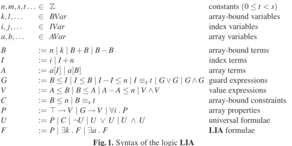
In order to build the constraint graph of a formula, one needs to pay attention to the following issue. Consider, e.g., the formula∀i, j.i − j ≤ 3 ∧ i ≡20∧ j ≡21→ a[i] −
b[ j] ≤ 5. The constraint graph of this formula needs to have a path of weight 5 between, e.g., a[0] and b[1], a[0] and b[3], a[0] and b[5], etc. As one can easily notice, the span of such paths is potentially unbounded. Since we would like this graph to represent a computation of a flat counter automaton, it is essential to define it as a sequence composed of (a possibly unbounded number of) repetitions of a finite number of (finite) sub-graphs (see, e.g., Fig. 2(a) or Fig. 2(b)). To this end, we introduce intermediary nodes which are connected between themselves with 0 arcs such that, for each non-local constraint of the form a[n] − b[m] ≤ w where |n − m| can be arbitrarily large, there exists exactly one path of weight w through these nodes. E.g., in Fig. 2(a), there is a path (a, 0)−→ (t5 ϕ, −3)→ . . .−0 −→ (t0 ϕ, 1)−→ (b, 1) for the constraint a[0]− b[1] ≤ 5, another path0
(a, 0)−→ (t5 ϕ, −3)→ . . .−0 −→ (t0 ϕ, 3)−→ (b, 3) for the constraint a[0] − b[3] ≤ 5, etc.0
Formally, the constraint graph ofϕ is Gι,ϕ= ,V, E- with the set of vertices V =
(
A
∪T
∪ {ζ}) × Z, whereA
= {a, b} are the array symbols in ϕ,T
= {tϕ} are theauxiliary symbols (tracks), andζ is a special symbol (zero track). The set of edges E is defined based on the type ofϕ, i.e. (F1)-(F3). For space reasons, we give here only the definitions for formulae of type (F3), which are the most interesting. Formulae (F1) and (F2) are treated in Appendix C. In general, for all types of formulae, we have:
E⊃ {(ζ, k)−→ (ζ, k + 1) | k ∈ Z} ∪ {(ζ, k + 1)0 −→ (ζ, k) | k ∈ Z}0 i.e., the value of the zero track stays constant.
Constraint graphs for (F3) formulae Letϕ be the formula below, where 0 ≤ s < t, 0≤ u < v, p ∈ Z∞, and q∈ Z : ∀i, j .^K1 k=1 f1 k≤ i ∧ L1 ^ l=1 i≤ g1 l ∧ i ≡st # $% & φ1 ∧ K2^ k=1 f2 k≤ j ∧ L2 ^ l=1 j≤ g2 l ∧ j ≡uv # $% & φ2 ∧ i − j ≤ p → a[i] − b[ j] ∼ q
Letφ1(i, k) and φ2( j, k) be the subformulae defining the ranges of i and j, respectively,
and
P
1the valuationι. Let T≤= {(tϕ, k)−→ (t0 ϕ, k + 1) | ∃n ∈
P
ι1∃m ∈P
ι2. n − m ≤ p} andT≤= {(tϕ, k)−→ (t0 ϕ, k − 1) | ∃n ∈
P
ι1∃m ∈P
ι2. n − m ≥ p}. Note that T≤and T≥areempty is the precondition ofϕ is not satisfiable. The set of edges E is defined by the following case split:
1. If p< ∞, we consider two cases, based on the direction of a[i] − b[ j] ∼ q: (a) for a[i] − b[ j] ≤ q, we have (Fig. 2(a)):
E⊃ {(a, k)−→ (tq ϕ, k − p) | k ∈
P
ι1} ∪ {(tϕ, k)−→ (b, k) | k ∈0P
ι2} ∪ T≤(b) for a[i] − b[ j] ≥ q, we have:
E⊃ {(b, k)−→ (t−q ϕ, k + p) | k ∈
P
ι2} ∪ {(tϕ, k)→ (a, k) | k ∈−0P
ι1} ∪ T≥2. If p= ∞, we consider again two cases, based on the direction of a[i] − b[ j] ∼ q: (a) for a[i] − b[ j] ≤ q, we have (Fig. 2(b)):
E⊃ {(a, k)−→ (tq ϕ, k) | k ∈
P
ι1} ∪ {(tϕ, k)−→ (b, k) | k ∈0P
ι2} ∪ T≤ ∪ T≥(b) for a[i] − b[ j] ≥ q, we have:
E⊃ {(b, k)−→ (t−q ϕ, k) | k ∈
P
ι2} ∪ {(tϕ, k)−→ (a, k) | k ∈0P
ι1} ∪ T≤ ∪ T≥ Nothing else is in E. ι(l1) ι(u1) a b tϕ 0 5 5 5 ι(u2) ι(l2) 0 0 0 0 0 0 0 0 0 0(a)∀i, j.l1≤ i ≤ u1∧l2≤ j ≤ u2∧i− j ≤ 3∧i ≡2
0∧ j ≡21→ a[i] − b[ j] ≤ 5 ι(l1) a 5 5 ι(u1) tϕ b 0 0 0 0 ι(l2) ι(u2) 0 0 0 0 (b)∀i, j.l1≤ i ≤ u1∧l2≤ j ≤ u2∧i ≡2 0∧ j ≡21→ a[i] − b[ j] ≤ 5
Fig. 2. Examples of constraint graphs for (F3) formulae
Relating constraint graphs and models of formulae Let us point out the correspon-dence between constraint graphs and models of formulae of the forms (F1)-(F3), i.e. if the vertices of a constraint graph for a formulaϕ can be labelled in a consistent way, then from the labelling one can extract a model forϕ and vice versa. This proves the correctness of the construction for constraint graphs, using the additional tracks.
Letϕ(k, a) be a formula of the forms (F1)-(F3), ι : k → Z a valuation of the array-bound variables inϕ, and Gι,ϕ= (V, E) its corresponding constraint graph. A labelling
Lab: V→ Z of Gι,ϕis called consistent if and only if (1) for all edges v1−→ vk 2∈ E, we
have Lab(v1) − Lab(v2) ≤ k and (2) Lab((ζ, n)) = 0 for all n ∈ Z.
Lemma 6. Letϕ(k, a) be a formula of the form (F1)-(F3). Then, for all valuations ι : k → Z and µ : a →ωZω, we have that ,ι, µ- |= ϕ if and only if there exists a
4.3 From Formulae to Counter Automata
In this section, we describe the construction of an FBCA Aϕcorresponding to a formula
ϕ such that (1) each run of Aϕcorresponds to a model ofϕ, and (2) for each model of ϕ,
Aϕhas at least one corresponding run. In this way, we effectively reduce the satisfiability
problem for LIA to the emptiness problem for FBCA.
The construction of FBCA is by induction on the structure of the formulae. For the rest of this section, letϕ be a formula, k the set of array-bound variables in ϕ, and a the set of array variables inϕ, i.e. FV (ϕ) = k ∪ a. Suppose that ϕ is the matrix of a formula in the normal form (NF), i.e. ϕ :W
i∈Iθi(k) ∧Vj∈Jψi j(k, a), where θi are
PA constraints andψi jare formulae of types (F1)-(F3). The automaton Aϕis defined as
U
i∈IAθi⊗ N
j∈JAψi j, where5 and ⊗ are the union and intersection operators on FBCA.
The construction of counter automata Aψi j for the formulaeψi jof type (F1)-(F3) relies
on the definition of the constraint graphs in Section 4.2. Namely, each accepting run of Aψi j gives a consistent valuation of the constraint graph ofψi j.
Counter Automata Templates. To simplify the definition of counter automata, we note that each constraint graph for the basic formulae of type (F1)-(F3) is composed of horizontal, vertical, and diagonal edges, which are defined in roughly the same way for all types of formulae (cf. Section 4.2). We take advantage of this fact, and we start by defining three types of counter automata templates, which are subsequently used to define the counter automata for the basic formulae.6More precisely, the automata for (F1)-(F3) formulae will be defined as⊗-products of particular instances of the automata templates for the horizontal, vertical, and diagonal edges of the appropriate constraint graphs. In the following definitions, we assume the existence of a special counter xτ
(tick), incremented by each transition rule, i.e. we suppose that the constraint x.τ= xτ+ 1
is implicitly in conjunction with each formula labelling a transition rule. Intuitively, the role of the xτcounter is to synchronism all automata composed by the⊗-product on a
common current position.
The template for the horizontal edges. Let a be an array symbol, dir∈ {left, right, bi} be a direction parameter, andφ be a formula on array-bound variables. Let xkbe the set
{xk| k ∈ FV (φ)}. We define the template H(a, dir, φ) = ,x, Q, L, R, −→-, where:
– x= {xa} ∪ xk. These counters will have the same names in all instances of H.
– Q= {qL, qR, pL, pR}. The control states are required to have fresh names in every
instance of H. L= {qL, pL} and R = {qR, pR}. – qL ξ − → qL, qR ξ − → qR, qL φ(xk) ∧ ξ −−−−−→ qR, pL ; −→ pL, pR ; −→ pR, and pL ¬φ(xk) −−−−→ pR.
In the above,φ(xk) is the formula obtained by replacing each occurrence of an
array-bound variable k∈ FV (φ) by its corresponding counter xk. The formulaξ(xa, x.a) is xa−
x.a≤ 0 if dir = right, x.a− xa≤ 0 if dir = left, and x.a= xaif dir= bi. Moreover, for
each transition rule, we assume the conjunctionV
k∈FV (φ)x.k= xkto be added implicitly
to the labelling formula, i.e. the value of an xkcounter stays constant throughout a run.
The xkparameters are used within guards of the form xτ∼ f (xk), where ∼∈ {≤, ≥} and
f is a linear combination of xk, in order to mark the position of the array boundaries,
during the run of the automata.
If, for a given valuation of the parameters xk, the formulaφ holds, then any
accept-ing run of (any instance of) H visits qLinfinitely often on the left, and qRinfinitely often
on the right. Otherwise, if for the given valuation of xk,φ does not hold, the instance
automata have a run that goes infinitely often through pLon the left, and through pRon
the right. In this case, the automata do not impose any constraints on xa.
The template for the diagonal edges. Let a, b be array symbols, q ∈ Z, p, s ∈ N+,
t∈ [0, s − 1], and dir ∈ {left, right} be a direction parameter. In the following, we refer to the sets L= {l1, . . . , lK} and U = {u1, . . . , uL} of lower, and respectively upper
bounds, where liand ujare linear combinations of array-bound variables, and let xk=
{xk| k ∈
SK
i=1FV(li) ∪
SL
j=1FV(uj)}. Further, we assume that L ∪ U 8= /0 – we deal
with the case of L∪ U = /0 later on. We define the template D(a, b, p, q, s,t, L, U, dir) = ,x, Q, L, R, −→-, where:
– x= {xa, xb} ∪ xk∪ {xi| 1 ≤ i < p}. The counters xa, xb, and xkwill have the same
names in all instances of D. On the other hand, the counters xi, 1≤ i < p, will
have fresh names in every instance of D. The xi counters are used for splitting
diagonal edges that span over more than one position, into series of diagonal edges connecting only adjacent positions.7
– Q= {qL, qR} ∪ {qi| 0 ≤ i < s} ∪ {qij| 0 ≤ j < s, j + 1 ≤ i < j + p}. The control
states are required to have fresh names in every instance of D. Let L= {qL} ∪
{qi| 0 ≤ i < s} and R = {qR} ∪ {qi| 0 ≤ i < s}.
– qL−→ q; L, qR−→ q; R, and qL ¬(∃i .V
l∈Li≥l(xk) ∧Vu∈Ui≤u(xk) ∧ i≡st)
−−−−−−−−−−−−−−−−−−−−−−−−−→ qR. – qL V l∈Lxτ≥l(xk)−1 ∧ (Wl∈Lxτ=l(xk)−1) ∧ xτ+1≡si −−−−−−−−−−−−−−−−−−−−−−−−−−−−−→ qi, for all 0≤ i < s. – qi V l∈Lxτ≥l(xk) ∧Vu∈Uxτ<u(xk) ∧ ξi[xa/x0,xb/xp]
−−−−−−−−−−−−−−−−−−−−−−−−−−−−→ q(i+1) mod s, for all 0≤ i < s.
– qi
W
u∈Uxτ=u(xk) ∧ xτ≡si∧ ξi[xa/x0,xb/xp]
−−−−−−−−−−−−−−−−−−−−−−−→ qi
i+1, for all 0≤ i < s.
– qi
W
u∈Uxτ=u(xk) ∧ xτ≡si∧ ξi[xa/x0,xb/xp]
−−−−−−−−−−−−−−−−−−−−−−−→ qR, for all 0≤ i < s, if p = 1.
– qij−−−−−−−−→ qξi[xa/x0,xb/xp] i+1j , for all 0≤ j < s, j < i < j + p − 1. – qj+p−1j −−−−−−−−→ qξi[xa/x0,xb/xp] R, for all 0≤ j < s, if p > 1.
In the above, l(xk) and u(xk) denote the expressions l and u in which each occurrence of
an array-bound variable k is replaced by its corresponding parameter xk. As before, for
each transition rule, we assume the conjunctionV
k∈FV (φ)x.k= xkto be added implicitly
to the labelling formula, i.e. we require that the value of an xk counter stays constant
throughout the run. The formulaeξiare defined as follows:
– if dir= right, ξi=Vk∈Kixk− x
.
k+1≤ αk, for Ki= {k | 0 ≤ k < p, i ≡sk+ t},
α0= q and αk= 0, k > 0,
7For instance, the constraint a[i] − b[i + 3] ≤ 5 can be split to a[i] − x
1[i + 1] ≤ 5, x1[i + 1] −
x2[i+2] ≤ 0, and x2[i+2]−b[i+3] ≤ 0. The constraints for array values of neighboring indices
can then be conveniently expressed by using the current and future values of the appropriate counters (e.g., for our example constraint, xa− x.1≤ 5, x1− x.2≤ 0, and x2− x.b≤ 0, which of
– if dir= left, ξi=Vk∈Kix
.
k−1− xk≤ αk, Ki= {k | 1 ≤ k ≤ p, k + i ≡st}, α1= q
andαk= 0, k > 1.
Finally, for the case L= U = /0, we define any instance of D(a, b, p, q, s,t, /0, /0, dir) to be A1⊗ A2, where A1is an instance of D(a, b, p, q, s,t, /0, {0}, dir) and A2is an instance
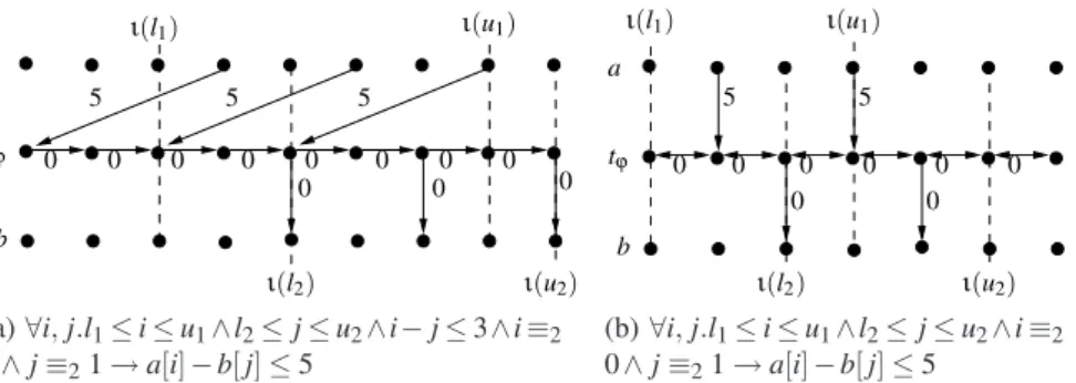
of D(a, b, p, q, s,t, {0}, /0, dir). qL qR q1 q1 2 q01 q02 q1 3 x.a− x1≤ 5 ; ; xτ≥ l1− 4 ∧ xτ= l1− 4 xτ ≥ l1− 4∧ xτ= l 1− 4 x.1− x2≤ 0 xτ≥ l1− 3 ∧ xτ< u1− 3 q0 ∧xτ≡20 xτ= u1− 3 x. a− x 1≤ 5 x.1− x2≤ 0 x.1− x2≤ 0 ∧ xτ≡21 xτ= u1− 3∧ ∧x. a− x1≤ 5 ∧x. 2− xtϕ≤ 0 ∧x. 1− x2≤ 0 xτ≥ l1− 3 ∧ xτ< u1− 3 ∧x. 2− xtϕ≤ 0 ∧x. 2− x tϕ≤ 0 ∧xτ + 1 ≡21 ∧xτ+ 1 ≡ 20 ∧x. a− x1≤ 5 ∧ x.2− xtϕ≤ 0 ¬(∃i . l1≤ i ≤ u1∧ i ≡20)
Fig. 3. The FBCA for the diagonal edges in the formulaϕ : ∀i, j.l1≤ i ≤ u1∧ l2≤ j ≤ u2∧ i − j ≤
3∧i ≡20∧ j ≡21→ a[i]−b[ j] ≤ 5 from Fig. 2(a) obtained as D(a,tϕ, 3, 5, 2, 0−3, {l1−3}, {u1−
3}, left). To understand the formula ξ0on the transition from q0to q1, note that the constraint
i≡sk+t in the definition of the set K0instantiates to 0≡2k− 3, and hence K0= {1, 3}. A similar
reasoning applies for the other transitions.
The construction can be understood by considering an accepting run of (any instance of) D. Let us consider the case in which there exists a value i in between the bounds that satisfies also the modulo constraint. If this is not the case, there will be an accepting run that takes the transition qL
¬(∃i .V
l∈Li≥l(xk) ∧Vu∈Ui≤u(xk) ∧ i≡st)
−−−−−−−−−−−−−−−−−−−−−−−−−→ qRexactly once.
Since the run is accepting, it must visit a state from L infinitely often on the left, and a state from R infinitely often on the right. There are three cases: (1) L8= /0 and U 8= /0, (2) L= /0 and U 8= /0, and (3) L 8= /0 and U = /0. In the case (1), a bi-infinite run will visit qL infinitely often on the left, and qR, infinitely often on the right. Notice that the run cannot
visit the loop q0−→ . . . −→ qs−1 infinitely often, due to the presence of both lower and
upper bounds on xτ. In the case (2), the run cannot take any of the transitions qL−→ qi,
0≤ i < s, due to the emptiness of L, which makes the guard unsatisfiable. Hence the only possibility for an accepting bi-infinite run is to visit the states q0−→ . . . −→ qs−1
infinitely often on the left. Due to the presence of the upper bound on xτ, the run cannot
stay forever inside this loop, and must exit via one of the qi−→ qii+1 (or qi−→ qRfor
p= 1) transitions, getting trapped into qRon the right. Case (3) is symmetric to (2).
Note that, in all cases, due to the modulo tests on xτin the entry and exit of the main
loop q0−→ . . . −→ qs−1on any accepting run, whenever a state qi, 0≤ i < s, is visited, the
value of the xτcounter must equal i modulo s. Note also that the role of the qijstates is
to describe constraints corresponding to edges that start inside the given interval bounds and lead above its upper bound (or vice versa). The number of such edges is bounded.
We do not use the same construction at the beginning of the interval, as the templates are applied such that none of the edges represented goes below the lower bounds. Template for the vertical edges. Let a, b be array symbols, q ∈ Z, p, s ∈ N+, and t∈ [0, s − 1]. We again refer to the sets L = {l1, . . . , lK} and U = {u1, . . . , uL} of lower,
and respectively upper bounds, where liand ujare linear combinations of array-bound
variables. Also, let xk= {xk| k ∈
SK
i=1FV(li) ∪ SLj=1FV(uj)}. Further, we assume
that L∪ U 8= /0 – we deal with the case of L ∪ U = /0 later on. We define the template V(a, b, p, q, s,t, L, U) = ,x, Q, L, R, −→-, where:
– x= {xa, xb} ∪ xk. The counters xa, xb, xkhave the same names in all instances of V .
– Q= {qL, qR} ∪ {qi| 0 ≤ i < s}. The control states are required to have fresh names
in every instance of V . L= {qL} ∪ {qi| 0 ≤ i < s} and R = {qR} ∪ {qi| 0 ≤ i ≤ s}.
– qL−→ q; L, qR−→ q; R, and qL ¬(∃i .V
l∈Li≥l(xk) ∧Vu∈Ui≤u(xk) ∧ i≡st)
−−−−−−−−−−−−−−−−−−−−−−−−−→ qR. – qL V l∈Lxτ≥l(xk)−1 ∧Wl∈Lxτ+1=l(xk) ∧ xτ+1≡si −−−−−−−−−−−−−−−−−−−−−−−−−−−−→ qi, 0≤ i < s. – qi V l∈Lxτ≥l(xk) ∧Vu∈Uxτ<u(xk) ∧ xa−xb≤q
−−−−−−−−−−−−−−−−−−−−−−−−−→ q(i+1) mod s, 0≤ i < s and i ≡st.
– qi
V
l∈Lxτ≥l(xk) ∧Vu∈Uxτ<u(xk)
−−−−−−−−−−−−−−−−−−→ q(i+1) mod s, 0≤ i < s and i 8≡st.
– qi W u∈Uxτ=u(xk) ∧ xτ≡si∧ xa−xb≤q −−−−−−−−−−−−−−−−−−−−→ qR, 0≤ i < s and i ≡st. – qi W u∈Uxτ=u(xk) ∧ xτ≡si −−−−−−−−−−−−−→ qR, 0≤ i < s and i 8≡st.
In the above, l(xk) and u(xk) denote the expressions l and u in which each occurrence of
an array-bound variable k is replaced by the parameter xk. As before, for each transition
rule, we assume the conjunctionV
k∈FV (φ)x.k= xkto be added implicitly to the labelling
formula, i.e. the value of an xk counter stays constant throughout the run. Finally, if
L= U = /0, we define any instance of V (a, b, p, q, s,t, /0, /0) as A1⊗ A2, where A1is an instance of V(a, b, p, q, s,t, /0, {0}) and A2is an instance of V(a, b, p, q, s,t, {0}, /0). The
intuition behind the construction of V is similar to the one of D.
4.4 Counter Automata for Basic Formulae
We are now ready to define the construction of FBCA for the basic formulae. This is done by composing instances of templates, using the⊗ operator for intersection (cf. Section 2). For space reasons, we only give here the construction of the FBCA for (F3) formulae. The formulae of type (F1), (F2), and PA constraints on array-bound variables are treated analogously in Appendix C. Letϕ be the (F3)-type formula:
∀i, j .^K1 k=1 fk1≤ i ∧ L1 ^ l=1 i≤ g1 l ∧ K2 ^ k=1 fk2≤ j ∧ L2 ^ l=1 j≤ g2 l ∧ i − j ≤ ∧ i ≡st∧ j ≡uv # $% & φ → a[i] − b[ j] ∼ q
where 0≤ s < t and 0 ≤ u < v. Let Li= { f1i, . . . , fKii} and Ui= {g
i
1, . . . , giLi}, for i = 1, 2,
respectively. By φ we denote the precondition of ϕ. The automaton Aϕ is defined as
p ∼ A1 A2 A3
∞ ≤ V (a,tϕ, q, s,t, L1, U1) H(tϕ, bi, ∃i, j.φ) V(tϕ, b, 0, u, v, L2, U2)
∞ ≥ V (b,tϕ, −q, u, v, L2, U2) H(tϕ, bi, ∃i, j.φ) V(tϕ, a, 0, s,t, L1, U1)
0 ≤ V (a,tϕ, q, s,t, L1, U1) H(tϕ, right, ∃i, j.φ) V (tϕ, b, 0, u, v, L2, U2)
0 ≥ V (b,tϕ, −q, u, v, L2, U2) H(tϕ, left, ∃i, j.φ) V(tϕ, a, 0, s,t, L1, U1)
> 0 ≤ D(a,tϕ, p, q, s,t − p, L1− p, U1− p, left) H(tϕ, right, ∃i, j.φ) V (tϕ, b, 0, u, v, L2, U2)
> 0 ≥ D(b,tϕ, p, −q, u, v, L2, U2, right) H(tϕ, left, ∃i, j.φ) V(tϕ, a, 0, s,t, L1, U1)
< 0 ≤ D(a,tϕ, −p, q, s,t, L1, U1, right) H(tϕ, right, ∃i, j.φ) V (tϕ, b, 0, u, v, L2, U2)
< 0 ≥ D(b,tϕ, −p, −q, u, v + p, L2+ p, U2+ p, left) H(tϕ, left, ∃i, j.φ) V(tϕ, a, 0, s,t, L1, U1)
Table 1. The instantiation table for (F3) formulae. Note that in some lines, we shift the original bounds appearing in the formula in order to be able to re-use the prepared templates that do not explicitly deal with edges leaving from within the given bounds and going below the lower bound. Due to the way the templates are constructed, the shifting preserves the semantics of the formula – instead of edges going below the lower bound of a certain interval, we obtain the same edges just going above the upper bound of the shifted interval, which our templates are prepared for. Given a set of integers S and an integer p, we use the notation S+ p for {s + p | s ∈ S}
4.5 From Formulae to Counter Automata
Given a formulaϕ(k, a) which is a positive boolean combination of formulae of types (F1)-(F3) and PA constraints on the array-bound variables k, let Aϕbe the automaton
defined inductively on the structure ofϕ as follows:
– ifϕ is of type (F1)-(F3), or a PA constraint on k, then Aϕis as in Section 4.4,
– ifϕ = ψ1∧ ψ2, then Aϕ= Aψ1⊗ Aψ2,
– ifϕ = ψ1∨ ψ2, then Aϕ= Aψ15 Aψ2.
Let r∈
R
(Aϕ) be an accepting run of Aϕandδ(r) = val(r(0))(xτ) be the value ofthe xτ (tick) counter at position 0 on r. We denote by η(r) = r ◦ σ−δ(r) the centered
runobtained from r by shifting it such that the value of xτ at position 0 is also 0. By
Lemma 1, r is an accepting run of Aϕif and only ifη(r) is. Notice that r induces the
following valuations on k and a, respectively:ιr(k) = val(η(r)(0))(xk), for all k ∈ k,
and µr(a, i) = val(η(r)(i))(xa), for all a ∈ a and i ∈ Z.
For an arbitrary valuationν ∈
V
(Aϕ), there exists r ∈R
(Aϕ) such that ν = val(r).Let Mϕ(ν) = ,ιr, µr- be the valuation of the free variables in ϕ that correspond to r. One
can see now that Mϕdefines a function Mϕ:
V
(Aϕ) → (k 4→ Z) × (a 4→ωZω).8Theorem 1. Letϕ(k, a) be a positive boolean combination of formulae of types (F1)-(F3) and PA constraints on the array-bound variables k, and Aϕ be the automaton
defined in the previous. Then, Mϕ(
V
(Aϕ)) = [[ϕ]].The proof is by induction on the structure ofϕ. For the base case, we use the cor-respondence between models and constraint graphs of formulae (F1)-(F3) (Lemma 6). The inductive step follows as a consequence of the fact that the class of FBCA is closed under union and intersection (Lemma 3). The main result of the paper is the following: Corollary 1. The logic LIA is decidable.
8By definition, for eachν ∈V(A
ϕ) there exist valuations ιr and µr, so Mϕ is defined for all
ν ∈V(Aϕ). Let r1, r2∈R(Aϕ) be two runs such that val(r1) = val(r2) = ν. We have δ(r1) =
The proof of Corollary 1 uses the normalization step (cf. Lemma 5) to rewrite any formula of LIA into the form (NF), and applies Theorem 1 to the matrix of the formula (i.e. the formula obtained by skipping the existential quantifier prefix).
5
Conclusions and Future Work
We present a new decidable logic for reasoning about properties of programs handling integer arrays. This logic allows to relate adjacent array values, as well as to express pe-riodic facts relating all values situated at equidistant positions. We establish decidability of this logic following the automata-theoretic approach. To this end, we define a new class of B¨uchi automata with counters, for which emptiness is decidable, and translate each formula into a corresponding automaton.
Future work will include the study of the complexity of our decision procedure and its implementation. We furthermore plan to develop invariant generation methods in order to give automatic correctness proofs for programs with integer arrays.
References
1. A. Armando, S. Ranise, and M. Rusinowitch. Uniform Derivation of Decision Procedures by Superposition. In Proc of CSL’01, LNCS 2142, 2001.
2. T. Arons, A. Pnueli, S. Ruah, J. Xu, and L.Zuck. Parameterized Verification with Automati-cally Computed Inductive Assertions. In CAV’01, LNCS 2102. Springer, 2001.
3. A. Bouajjani, Y. Jurski, and M. Sighireanu. A Generic Framework for Reasoning About Dynamic Networks of Infinite-State Processes. In TACAS’07, LNCS 4424. Springer, 2007. 4. M. Bozga, R. Iosif, and Y. Lakhnech. Flat Parametric Counter Automata. In Proc. of
ICALP’06, LNCS 4052. Springer, 2006.
5. A.R. Bradley, Z. Manna, and H.B. Sipma. What ’s Decidable About Arrays? In Proc. of VMCAI’06, LNCS 3855. Springer, 2006.
6. H. Comon and Y. Jurski. Multiple Counters Automata, Safety Analysis and Presburger Arith-metic. In Proc. of CAV’98, LNCS 1427. Springer, 1998.
7. S. Ghilardi, E. Nicolini, S. Ranise, and D. Zucchelli. Decision Procedures for Extensions of the Theory of Arrays. Annals of Mathematics and Artificial Intelligence, 50, 2007.
8. P. Habermehl, R. Iosif, and T. Vojnar. What else is decidable about integer arrays? Technical Report TR-2007-8, Verimag, 2007.
9. J. Jaffar. Presburger Arithmetic with Array Segments. Inform. Proc. Letters, 12, 1981. 10. J. King. A Program Verifier. PhD thesis, Carnegie Mellon University, 1969.
11. P. Mateti. A Decision Procedure for the Correctness of a Class of Programs. Journal of the ACM, 28(2), 1980.
12. J. McCarthy. Towards a Mathematical Science of Computation. In IFIP Congress, 1962. 13. M.L. Minsky. Computation: Finite and Infinite Machines. Prentice-Hall, Inc., 1967. 14. M. Nivat and D. Perrin. Ensembles reconnaissables de mots biinfinis. Canad. J. Math.,
38:513–537, 1986.
15. M. Presburger. Uber die Vollst¨andigkeit eines gewissen Systems der Arithmetik ganzer¨ Zahlen, in welchem die Addition als einzige Operation hervortritt. In Comptes Rendus du Premier Congr`es des Math´ematiciens des Pays Slaves, pages 92–101, Warsaw, Poland, 1929. 16. A. Stump, C.W. Barrett, D.L. Dill, and J.R. Levitt. A Decision Procedure for an Extensional
Theory of Arrays. In Proc. of LICS’01, 2001.
17. N. Suzuki and D. Jefferson. Verification Decidability of Presburger Array Programs. Journal of the ACM, 27(1), 1980.
18. W. Thomas. Automata on Infinite Objects. In Handbook of Theoretical Computer Science, volume B: Formal Models and Semantics. Elsevier, 1990.
A
Extensions of Flat Counter Automata
In [6, 4] it is shown that given a flat counter automaton A= ,x, Q, −→-, and a loop γ on a control state q∈ Q, labelled with DBM formulae only, one can effectively build a PA formulaΨq,γ(y, x, x.) which is satisfied by all triples ,n, v, v.-, where there exists an
execution corresponding to n loop iterations, in which the initial values of the counters are v and the final values are v.. Based on this, we prove two important lemmas whose proofs can be found in [8].
Lemma 7. If any control loop of A is labelled by a parametric DBM formula, then for any two control states q, q.∈ Q, one can effectively build a PA formula Rq,q.(x, x.) such
that, for any two configurations(q, ν) and (q., ν.), (q., ν.) is a successor of (q, ν) if and only if|= Rq,q.(ν(x), ν.(x.)).
Lemma 8. Given a control loopγ labelled by a parametric DBM formula, and a control state q onγ, one can effectively build a PA formula Iq,γ(x), such that, for any
configura-tion(q, ν), there exists an infinite computation along γ, starting with (q, ν) if and only if|= Iq,γ(ν(x)).
B
Verification Conditions for an Array Merging Example
Consider the following program that takes two arrays a and b, and merges their first n elements by alternating elements from a with elements from b. Suppose, moreover, that the first n elements of a are less than or equal to the first n elements of b. The resulting array will have all its first n elements on even positions less than or equal to the first n elements on odd positions.
{{ n > 0 ∧ ∀i, j . 0 ≤ i, j < n → a[i] ≤ b[j] }} for (k=0, l=0; k< n; k++, l+=2) {{ n > 0 ∧ k ≤ n ∧ l = 2k ∧ ∀i, j . 0 ≤ i, j < 2k ∧ i ≡20 ∧ j ≡21→ c[i] ≤ c[j] ∧ ∀i, j . 0 ≤ i, j < n → a[i] ≤ b[j] }} { c[l] = a[k]; c[l + 1] = b[k];} {{ n > 0 ∧ ∀i, j . 0 ≤ i, j < 2n ∧ i ≡20 ∧ j ≡21→ c[i] ≤ c[j] }}
The pre-, post-condition, and loop invariant needed for the proof of this program are annotated directly into the program text using double curly braces. We show in the following that the verification conditions to be checked to prove the correctness of the program fall into our logic, and so they are decidable.
We need to check three verification conditions corresponding to the initialisation of the loop, the loop body, and the finalisation of the loop.
The initialisation consists of the two unconditional assignment statements k=0 and l=0. We need to check that the following formula is logically valid (we use primed names of variables to distinguish the current and future values of the variables):
∀ a,a., b, b., c, c., n, n., k, k., l, l..
n> 0 ∧ (∀i, j . 0 ≤ i, j < n → a[i] ≤ b[ j]) ∧ k.= 0 ∧ l.= 0 ∧ n.= n ∧ (∀i . a.[i] = a[i]) ∧ (∀i . b.[i] = b[i]) ∧ (∀i . c.[i] = c[i])
−→
n.> 0 ∧ k.≤ n. ∧ l.= 2k.∧
(∀i, j . 0 ≤ i, j < 2k. ∧ i ≡20∧ j ≡21→ c.[i] ≤ c.[ j]) ∧
(∀i, j . 0 ≤ i, j < n → a.[i] ≤ b.[ j])
However, checking the validity of the above formula is equal to checking that its nega-tion, which clearly fits our logic, is unsatisfiable:
∃ a,a., b, b., c, c., n, n., k, k., l, l..
n> 0 ∧ (∀i, j . 0 ≤ i, j < n → a[i] ≤ b[ j]) ∧ k.= 0 ∧ l.= 0 ∧ n.= n ∧ (∀i . a.[i] = a[i]) ∧ (∀i . b.[i] = b[i]) ∧ (∀i . c.[i] = c[i])
∧
(n.≤ 0 ∨ k.> n. ∨ l.< 2k. ∨ l.> 2k.∨
(∃i, j . 0 ≤ i, j < 2k. ∧ i ≡20∧ j ≡21∧ c.[i] > c.[ j]) ∨
(∃i, j . 0 ≤ i, j < n ∧ a.[i] > b.[ j]))
To see this, note that the existentially quantified index variables in the last two lines of the above formula can be given unique names and the appropriate quantifiers moved to the prefix of the formula.
To check the effect of the loop body, i.e. the assignments c[l] = a[k], c[l+1] = b[k], k++, and l+=2 which are executed provided that k<n, we have to prove that the follow-ing holds: ∀ a,a., b, b., c, c., n, n., k, k., l, l.. n> 0 ∧ k ≤ n ∧ l = 2k ∧ (∀i, j . 0 ≤ i, j < 2k ∧ i ≡20∧ j ≡21→ c[i] ≤ c[ j]) ∧ (∀i, j . 0 ≤ i, j < n → a[i] ≤ b[ j]) ∧ k< n ∧ k.= k + 1 ∧ l.= l + 2 ∧ n.= n ∧ (∀i . a.[i] = a[i]) ∧ (∀i . b.[i] = b[i]) ∧
(∀i . i < l → c.[i] = c[i]) ∧ (∀i . i > l + 1 → c.[i] = c[i]) ∧
c.[l] = a[k] ∧ c.[l + 1] = b[k] −→ n.> 0 ∧ k.≤ n. ∧ l.= 2k.∧ (∀i, j . 0 ≤ i, j < 2k. ∧ i ≡ 20∧ j ≡21→ c.[i] ≤ c.[ j]) ∧ (∀i, j . 0 ≤ i, j < n → a.[i] ≤ b.[ j])
Again, checking the validity of the above formula is equal to checking that its negation, is unsatisfiable: ∃ a,a., b, b., c, c., n, n., k, k., l, l.. n> 0 ∧ k ≤ n ∧ l = 2k ∧ (∀i, j . 0 ≤ i, j < 2k ∧ i ≡20∧ j ≡21→ c[i] ≤ c[ j]) ∧ (∀i, j . 0 ≤ i, j < n → a[i] ≤ b[ j]) ∧ k< n ∧ k.= k + 1 ∧ l.= l + 2 ∧ n.= n ∧ (∀i . a.[i] = a[i]) ∧ (∀i . b.[i] = b[i]) ∧
(∀i . i < l → c.[i] = c[i]) ∧ (∀i . i > l + 1 → c.[i] = c[i]) ∧
c.[l] = a[k] ∧ c.[l + 1] = b[k] ∧
(n.≤ 0 ∨ k.> n. ∨ l.< 2k. ∨ l.> 2k.∨
(∃i, j . 0 ≤ i, j < 2k. ∧ i ≡20∧ j ≡21∧ c.[i] > c.[ j]) ∨
(∃i, j . 0 ≤ i, j < n ∧ a.[i] > b.[ j]))
Finally, in order to check the finalisation of the loop (i.e. the exit of the loop when k≥ n), one has to check the validity of the following formula:
∀ a,a., b, b., c, c., n, n., k, k., l, l.. n> 0 ∧ k ≤ n ∧ l = 2k ∧
(∀i, j . 0 ≤ i, j < 2k ∧ i ≡20∧ j ≡21→ c[i] ≤ c[ j]) ∧
(∀i, j . 0 ≤ i, j < n → a[i] ≤ b[ j]) ∧ k≥ n ∧ k.= k ∧ l.= l ∧ n.= n ∧
(∀i . a.[i] = a[i]) ∧ (∀i . b.[i] = b[i]) ∧ (∀i . c.[i] = c[i]) ∧
−→
n.> 0 ∧ (∀i, j . 0 ≤ i, j < 2n. ∧ i ≡20∧ j ≡21→ c.[i] ≤ c.[ j])
Like in the previous cases, checking the validity of the above formula is equal to check-ing that its negation is unsatisfiable:
∃ a,a., b, b., c, c., n, n., k, k., l, l.. n> 0 ∧ k ≤ n ∧ l = 2k ∧
(∀i, j . 0 ≤ i, j < 2k ∧ i ≡20∧ j ≡21→ c[i] ≤ c[ j]) ∧
(∀i, j . 0 ≤ i, j < n → a[i] ≤ b[ j]) ∧ k≥ n ∧ k.= k ∧ l.= l ∧ n.= n ∧
(∀i . a.[i] = a[i]) ∧ (∀i . b.[i] = b[i]) ∧ (∀i . c.[i] = c[i]) ∧ ∧
(n.≤ 0 ∨ (∃i, j . 0 ≤ i, j < 2n. ∧ i ≡20∧ j ≡21∧ c.[i] > c.[ j]))
C
Constraint Graphs and Counter Automata for (F1) and (F2)
Here we define the constraint graphs for formulae of type (F1) and (F2) and the cor-responding counter automata as well as the automaton for Presburger bound constraint formulae.
C.1 Constraint graphs
Formulae of type (F1) Letϕ be the formula ∀i .^K k=1 fk≤ i ∧ L ^ l=1 i≤ gl∧ i ≡st # $% & φ → a[i] ∼ h(k)
where 0≤ t < s. Let
P
ι= {n ∈ Z | |= φι[n/i]}.The set of edges E is defined by the following case split:
1. If the right hand side of the implication is a[i] ≤ h(k), we have (cf. Figure 4): E⊃ {(a, k)−−→ (ζ, k) | k ∈h(k)
P
ι}2. Otherwise, if the right hand side of the implication is a[i] ≥ h(k), we have: E⊃ {(ζ, k)−−−→ (a, k) | k ∈−h(k)
P
ι}0 0 0 0 0 0 a ζ h(k) h(k) h(k) Lι Uι
Fig. 4. Constraint graph for∀i . l ≤ i ≤ u ∧ i ≡20→ a[i] ≤ h(k)
Formulae of type (F2) Letϕ be the formula: ∀i .^K k=1 fk≤ i ∧ L ^ l=1 i≤ gl∧ i ≡st # $% & φ → a[i] − b[i + p] ∼ q
where 0≤ s < t, p ∈ N, and q ∈ Z. Let
P
ι= {n ∈ Z | |= φι[n/i]}.The set of edges E is defined by the following case split:
1. If the right hand side of the implication is a[i] − b[i + p] ≤ q, we have (cf. Fig. 5): E⊃ {(a, k)−→ (b, k + p) | k ∈q
P
ι}a
b
5 5 5
Lι Uι
Fig. 5. Constraint graph for∀i.l ≤ i ≤ u ∧ i ≡20→ a[i] − b[i + 3] ≤ 5
2. If the right hand side of the implication is a[i] − b[i + p] ≥ q, then E ⊃ {(b, k + p)−→ (a, k) | k ∈−q
P
ι}Nothing else is in E.
C.2 Counter Automata Formulae of type (F1) Letϕ be
∀i . K ^ k=1 fk≤ i ∧ L ^ l=1 i≤ gl ∧ i ≡st→ a[i] ∼ h(k)
where 0≤ t < s. Let L = { f1, . . . , fK} and U = {g1, . . . , gL}. Then we define Aϕ=
(a) ∼ A1 A2 ≤ V (a, ζ, h, s,t, L, U) H(ζ, bi, ;) ≥ V (a, ζ, −h, s,t, L, U) H(ζ, bi, ;) (b) p ∼ Aϕ 0 ≤ V (a, b, q, s,t, L, U) 0 ≥ V (b, a, −q, s,t, L, U) > 0 ≤ D(a, b, p, q, s,t, L, U, right) > 0 ≥ D(b, a, p, −q, s,t, L, U, left) < 0 ≤ D(a, b, −p, q, s,t + p, L + p, U + p, left) < 0 ≥ D(b, a, −p, −q, s,t + p, L + p, U + p, right) Table 2. The instantiation table for (F1) and (F2) formulae
Formulae of type (F2) Letϕ be the formula : ∀i . K ^ k=1 fk≤ i ∧ L ^ l=1 i≤ gl ∧ i ≡st→ a[i] − b[i + p] ∼ q
where 0≤ s < t. As previously, we denote L = { f1, . . . , fK} and U = {g1, . . . , gL}. The
instantiation of Aϕis done according to the value of p and∼ as described in Table 2(b).9
Given a set of integers S and an integer p we use the notation S+ p for {s + p | s ∈ S}. Counter Automata for Array-Bound Constraints. The FBCA Aθfor a Presburger
constraint θ on array-bound variables is Aθ= ,xk, Q, L, R, −→-, where xk is the set
{xk | k ∈ FV (θ)}, Q = {qL, qR}, L = {qL}, R = {qR}, and −→= {qL−→ q; L, qL θ(xk)
−−−→ qR, qR
;
−→ qR}, and θ(xk) denotes the formula θ in which each occurrence of an
array-bound variable k∈ FV (θ) is replaced by its corresponding parameter xk.
D
Proofs
Proof of Lemma 1 Let A= ,x, Q, L, R, −→-. “⇒” r is left-accepting iff there exists an infinite decreasing sequence. . . i3< i2< i1< 0 of positions in r, visiting a control state
from L. This implies that i3− 1 < i2− 1 < i1− 1 < 0 visits the same control state, hence
r◦ s is left-accepting. r is right-accepting iff there exists an infinite increasing sequence 0< j1< j2< j3< . . . of positions in r, which visits a control state from R. But this
implies that 0< j2− 1 < j3− 1 < . . . visits the same state from R, hence r ◦ s is
right-accepting. “⇐” This direction follows a similar argument. BC 9Note that in the last two lines of Table 2(b), we shift the original bounds appearing in the
formula in order to be able to re-use the prepared templates that do not explicitly deal with edges leaving from within the given bounds and going below the lower bound. Due to the way the templates are constructed, the shifting preserves the semantics of the formula – instead of edges going below the lower bound of a certain interval, we obtain the same edges just going above the upper bound of the shifted interval, which our templates are prepared for.
Proof of Lemma 2 The proof uses the results of Appendix A, namely Lemmas 7 and 8. Let A= ,x, Q, L, R, −→- be a FBCA. W.l.o.g. we can assume that any control state q ∈ L∪ R belongs to exactly one elementary cycle. For, if q does not belong to a cycle, it cannot occur infinitely often on a run. Moreover, if q belongs to two or more elementary cycles, then A is not flat, in contradiction with the definition of FBCA. Let l∈ L and r∈ R be fixed for the rest of this proof. We construct a Presburger formula Φl,rwhich is
satisfiable if and only if there exists a bi-infinite run that visits l infinitely often on the left and r infinitely often on the right.
Letγ be the elementary cycle to which l belongs, and←γ be the cycle obtained by reversing each transition q−→ qϕ . into q. ϕ
.
−→ q, where ϕ. is obtained fromϕ by inter-changing the occurrences of the counters in x with x., and vice versa. Let Il,←
γ(x) be
the Presburger formula defining the set of valuationsν for which there exists an infinite computation along←γ starting in (l, ν).
Letδ be the elementary cycle to which r belongs, and Ir,δ(x) be the Presburger
formula defining the set of valuationsν for which there exists an infinite computation alongδ starting in (r, ν). The formula encoding the existence of a bi-infinite run that visits l infinitely often on the left and r infinitely often on the right, is the following:
Φl,r:∃x∃x.. Il,←
γ(x) ∧ Rl,r(x, x .) ∧ I
r,δ(x.)
The proof thatΦl,ris satisfiable if and only if
R
(A) 8= /0 comes as an immediateconse-quence of the meaning of the Il,←
γ, Rl,rand Ir,δformulae. BC
Proof of Proposition 1 The direction
R
(A) ⊆R
(Ac) is trivial, since L ⊆ Lcand R⊆ Rc.To prove the fact that
R
(A) ⊇R
(Ac), let r be an accepting run of Ac. Then there existsa state q∈ Lcthat repeats infinitely often on the left in r. There are two situations: either
q∈ L, in which case r is directly left-accepting for A, or there exists a state q.∈ L which belongs to the same elementary cycle as q in A. By the flatness of A, this means that q. will be visited infinitely often on the left as well. Analogously, one proves that r is a
right-accepting run of A. BC
Proof of Lemma 3 The proof for closure under union is trivial. We will give the proof for closure under intersection in the following.
Let Ai = ,xi, Qi, Li, Ri, →i-, i = 1, 2 be two FBCA, and A = ,x, Q, L, R, −→- be their
product, i.e. A= A1⊗ A2.
1. We first prove that A belongs to the class FBCA. For this we need to show that each control state of A belongs to at most one elementary cycle. For an arbitrary state (q, q.) ∈ Q
1× Q2, let pr1((q, q.)) = q, pr2((q, q.)) = q.and for an arbitrary cycleγ in
A, let pri(γ) denote the corresponding cycles in Ai, obtained by projection of the i-th
control state, i= 1, 2. Suppose that there is a control state (q, q.) ∈ Q
1× Q2that belongs
to (at least) two different elementary cycles,γ and δ. Then q belongs to pr1(γ) and
and A2are flat, then pri(γ) and pri(δ) must be (possibly trivial) unfoldings of the same
elementary cycleεi in Ai, for i= 1, 2, respectively. In other words, pri(γ) = ki· εiand
pri(δ) = li· εi, for i= 1, 2 and ki, li∈ N.
Let m be the least common multiple of|ε1| and |ε2|, and ni=|εmi|, for i= 1, 2. Let
α be the cycle in A obtained by the composition of the two cycles obtained by iterating ε1 n1 times, and ε2 n2 times, respectively, i.e. pri(α) = ni· εi, i= 1, 2. Since εi are
elementary cycles of Ai, it follows thatα is the smallest cycle of A with the property
that pri(α) is an unfolding of εi. Henceγ and δ, must both be either α or unfoldings of
α, contradicting the assumption that they were different elementary cycles of A. To prove that the elementary cycles of A are labelled with (parametric) DBM for-mulae only, notice that any cycle of A is a composition of two (unfoldings of) cycles in A1and A2. Since both component cycles are labelled with DBM formulae, and the
label of the transitions of A is the conjunction of the labels of the transitions in A1, A2,
it follows that the resulting cycle is labelled with DBM formulae as well. 2. Second, we prove that
V
(A) =V
(A1) ↑x1∪x2 ∩V
(A2) ↑x1∪x2.Let s∈
V
(A1)↑x1∪x2 ∩V
(A2)↑x1∪x2be a bi-infinite sequence of counter valuations.From the definition of
V
(.), there exist r1∈R
(A1) and r2∈R
(A2) such that val(r1) =s↓x1and val(r2) = s ↓x2.
Let i∈ Z be an arbitrary position, and r1(i) = (q1, ν1), r1(i + 1) = (q.1, ν.1), r2(i) =
(q2, ν2), r.2(i + 1) = (q2., ν.2) be successive configurations of r1 and r2, respectively,
whereν1, ν.1 : x1→ Z and ν2, ν.2 : x2→ Z are valuations of x1, x2. Then there exist
transition rules q1
ϕ1(x1,x.1)
−−−−−→ q.1in A1, and q2
ϕ2(x2,x.2)
−−−−−→ q.2in A2, such thatϕ1(ν1(x1), ν.1(x.1))
andϕ2(ν2(x2), ν.2(x.2)) are both valid. Hence, by construction of A, there exists a
tran-sition rule (q1, q2) ϕ1∧ϕ2
−−−→ (q.
1, q.2), such that ϕ1∧ ϕ2 is satisfied by (ν1∪ ν.1) ↑x1∪x2
∩(ν2∪ ν.2)↑x1∪x2. In this way, one can build a bi-infinite run r of A, such that val(r) = s.
It remains to be proven that this run is an accepting run of A.
Since ri is an accepting run of Ai, then by Proposition 1, it is also an accepting
run of Aci, for i= 1, 2. By the flatness of A1, and, implicitly of Ac1, there exist a
se-quence σ1 of states from Lc1 that repeats infinitely often to the left of r1, i.e. there
exists a position k1∈ Z, such that the restriction of r1 to (−∞, k1] is of the form
. . . σ1σ1. Analogously, there exists a sequence σ2 of states from Lc2, and a position
k2∈ Z such that the restriction of r2 to(−∞, k2] is of the form . . . σ2σ2. Then, the
restriction of r to (−∞, min(k1, k2)] is of the form . . . σσ, where σ is a sequence of
pairs(q, q.) ∈ Lc
1× Lc2. Hence there exists such a pair repeating infinitely often to the
left in r, i.e. r is left-accepting. Analogously, one proves that r is right-accepting. We have proved that
V
(A) ⊇V
(A1) ↑x1∪x2 ∩V
(A2) ↑x1∪x2. The directionV
(A) ⊆V
(A1) ↑x1∪x2 ∩V
(A2) ↑x1∪x2is proved using a similar argument. BCProof of Lemma 4 This can be proven by a reduction from the halting problem for 2-counter automata [13]. A 2-counter machine with non-negative counters c1, c2is a
sequential program:
![Fig. 3. The FBCA for the diagonal edges in the formula ϕ : ∀i, j.l 1 ≤ i ≤ u 1 ∧ l 2 ≤ j ≤ u 2 ∧ i− j ≤ 3∧i ≡ 2 0∧ j ≡ 2 1 → a[i]− b[ j] ≤ 5 from Fig](https://thumb-eu.123doks.com/thumbv2/123doknet/14520145.531254/13.892.200.715.300.497/fig-fbca-diagonal-edges-formula-ϕ-i-fig.webp)
![Fig. 5. Constraint graph for ∀i.l ≤ i ≤ u∧ i ≡ 2 0 → a[i]− b[i + 3] ≤ 5](https://thumb-eu.123doks.com/thumbv2/123doknet/14520145.531254/20.892.290.640.571.661/fig-constraint-graph-i-l-i-u-i.webp)
