An Approximate integral method for calculating the diffracted component from multiple two-dimensional objects

Publisher’s version / Version de l'éditeur:

Journal of the Acoustical Society of America, 97, 1, pp. 51-61, 1995-01-01

READ THESE TERMS AND CONDITIONS CAREFULLY BEFORE USING THIS WEBSITE.

https://nrc-publications.canada.ca/eng/copyright

Vous avez des questions? Nous pouvons vous aider. Pour communiquer directement avec un auteur, consultez la première page de la revue dans laquelle son article a été publié afin de trouver ses coordonnées. Si vous n’arrivez pas à les repérer, communiquez avec nous à PublicationsArchive-ArchivesPublications@nrc-cnrc.gc.ca.

Questions? Contact the NRC Publications Archive team at

PublicationsArchive-ArchivesPublications@nrc-cnrc.gc.ca. If you wish to email the authors directly, please see the first page of the publication for their contact information.

NRC Publications Archive

Archives des publications du CNRC

This publication could be one of several versions: author’s original, accepted manuscript or the publisher’s version. / La version de cette publication peut être l’une des suivantes : la version prépublication de l’auteur, la version acceptée du manuscrit ou la version de l’éditeur.

Access and use of this website and the material on it are subject to the Terms and Conditions set forth at

An Approximate integral method for calculating the diffracted

component from multiple two-dimensional objects

Nightingale, T. R. T.

https://publications-cnrc.canada.ca/fra/droits

L’accès à ce site Web et l’utilisation de son contenu sont assujettis aux conditions présentées dans le site LISEZ CES CONDITIONS ATTENTIVEMENT AVANT D’UTILISER CE SITE WEB.

NRC Publications Record / Notice d'Archives des publications de CNRC:

https://nrc-publications.canada.ca/eng/view/object/?id=5c92a99f-77c5-4d78-a8bd-3ac22150a033 https://publications-cnrc.canada.ca/fra/voir/objet/?id=5c92a99f-77c5-4d78-a8bd-3ac22150a033

http://www.nrc-cnrc.gc.ca/irc

An Approx im a t e int e gra l m e t hod for c a lc ula t ing t he diffra c t e d

c om pone nt from m ult iple t w o-dim e nsiona l obje c t s

N R C C - 3 5 9 8 6

N i g h t i n g a l e , T . R . T .

J a n u a r y 1 9 9 5

A version of this document is published in / Une version de ce document se trouve dans:

Journal of the Acoustical Society of America,

97, (1), pp. 51-61, January 01,

1995

The material in this document is covered by the provisions of the Copyright Act, by Canadian laws, policies, regulations and international agreements. Such provisions serve to identify the information source and, in specific instances, to prohibit reproduction of materials without written permission. For more information visit http://laws.justice.gc.ca/en/showtdm/cs/C-42

Les renseignements dans ce document sont protégés par la Loi sur le droit d'auteur, par les lois, les politiques et les règlements du Canada et des accords internationaux. Ces dispositions permettent d'identifier la source de l'information et, dans certains cas, d'interdire la copie de documents sans permission écrite. Pour obtenir de plus amples renseignements : http://lois.justice.gc.ca/fr/showtdm/cs/C-42

·

lV',Rcc-

ＳＵＧＱｧｾ

An approximate integral method. for calculating the diffracted

component from multiple two-dimensional objects

T. R. T. Nightingale

Acoustics Laboratory, Institute for Research in Construction, National Researchｃｯｵｮ｣ｩｾ Ottawa K1AOR6, Canada

(Received 24 March 1993; accepted for publication 25 August 1994)

A method for determining the diffracted or scattered components due to the in.!et-actiollc"fｾ wave with multiple two-dimensional objects is given. The method presented uses approximate boundary conditions to simplify the numerically cumbersome set of integral equations associated with nonapproximate analytic solutions of the Helmholtz integral. The approximate boundary conditions, defined here, are shown to decouple the N by N set of simultaneous equations. The approximate boundary condilions are used to calculate the insertion loss for various sizes of two-dimensional objects. The predictions are compared to measured results and limitations are discussed.

PACS numbers: 43.20.Fn

gral methods usually give bounded results correct to within an order of maguitude, even when the boundary conditions are clearly not satisfied. Furthermore, the object can be a plane of any dimension. Figure 1 shows the source, screen, and receiver locations Used in the insertion loss measure-ments. Figure 2 shows the errors associated with the calcu-lation of the scattered field due to a screen of finite dimen-sioll using approximate methods. The geometric uniform theory of diffraction completely fails to predict the correct insertion loss for the low frequencies. In fact, due to its as-ymptotic formulation, the insertion loss is diverging to infin-ity as the frequency approaches zero. Clearly, applying the geometrical method to a multiple screen diffraction problem involving objects of this size would lead to a compounding of significant errors. For the cases when geometrical methods fail, a· multiple screen diffraction model based on the ap-proximate integral method would be most useful. However, the approximate integral methods are restricted to describing only single planar objects. The KBCs would have to be modified to make allowances for the description of the total field on more than one screen or aperture.

The analytic methods offer a more general solution to radiation problems as they solve the reduced wave equation over the object's surface without approximation (I.e., with an unapproximated set of boundary conditions). However, methods using this technique are not without limitations, as will be discussed briefly after the introduction of the Helm-holtz integrals upon which they are based.

Let the surface of the object be denoted by 8D,its inte-rior volume byD,and its exterior region byE, as shown in Fig. 3. Equation(1)5 defines the velocity potential<Pin terms of known boundary conditions,

INTRODUCTION I

The scattered field due to the presence of an object may be calculated by two groups of methods: approximate or ana-lytic. Each group is formed from the Helmholtz integral equation. The limitations of each method is manifest in its formulation. These will be briefly discussed to illustrate the need for an alternate method that is capable of describing the diffracted field

liue

to multiple two-dimensional objects, when the geometrical methods fail and when the computing time of the analytic methods becomes excessive.

The following is a list of acronyms that will be used throughout the discussions:

(1) KBC-Kirchhoff boundary conditions, (2) ill-Helmholtz integral,

(3) HKI-Helmholtz-Kirchhoff integral, (4) RKI-Rayleigh-Kirchhoff integral, and

(5) MKBC-modified Kirchhoff boundary conditions. In this paper screens are two-dimensional objects or "thin" three-dimensional objects that can be considered as behaving like two-dimensional objects for the wavelengths considered.

There are two types of approximate methods: the geo-metrical theories of diffraction, and approximate integral so-lutions using the Kirchhoff boundary conditions. Each re-quires that a specific set of conditions be satisfied. The geometrical theories of diffraction (Keller's geometrical theory of diffraction,l and Kouyoujian and Pathak's uniform theory of diffraction2) which invoke a high-frequency

ap-p'!:oximation are restricted to objects that can be constructed from one or more semi-infinite half-planes. Description of ｾ｣｡ｴｴ･ｲ･､ fields due to simple objects of finite extent using geometrical methods can lead to very substantial errors as the solution fails to converge if restrictions on object dimen-sion, source-object, and object-receiver distances are not' satisfied.3 Approximate integral methods, which include the HKIs and RKIs, are also based on a high-frequency approximation-the KBCs.4

Unlike the geometrical theories, the approximate

inte-f inte-f[

A. ( )0 G(p,q) G( )0 <P,(q)]d '1', q

on

p,q

on

Sq. q q 8D { <p,(p)- <Po(p), peE, = O<p,(p)- <Po(p), pe8D, -<po(p), peD, (la)

(2c)

Exterior E

FIG. 3. Solid object and its surfaces used in the discussion.

21Tf k =

-c '

Interior 0

Surface

ro

where

f

and c are the frequency and velocity of the wave in free space, respectively.

Typically, Eq. (1) is used ina two-pass process to deter-mine the field at an arbitrary point in space. First, the surface distribution is determined using Eq.(1)(pEaD) subject to a

set of boundary conditions. Once the surface distribution is known, then it is possible to compute the field for an arbi-trary point

in

free space (p EE), again using Eq. (1). Gen-erally, there is no closed-form solution for a body of arbitrary shape. Consequently, the surface distribution is computed over enough points so that the premise for numerical integra-tion remains valid, Le., magnitude and phase are approxi-mately constant over the area element. For high frequencies, where the magnitude and phase may vary significantly with small changes in distance, a very large nU!T'':-er of integration points may have to be L:.ed, resulting in excessive computa-tion times.

Solving

Eq.

(1) subject to a complete set of boundary conditions is known as the Helmholtz integral equation method (HIEM). For infinitely thin rigid planar objects, the method requires treatment of a very singular pole, third or-der, in the domain of integration. Terai3 has shown that this can be treated as the sum of three terms which do not require special attention. The HIEM applied to a noninfinitely thin object (Le., ｴｨｲ･･ｾ､ｩｭ･ｮｳｩｯｮ｡ｬＩ suffers from nonuniqueness that occurs at frequencies that correspond to the characteris-tic frequencies of the internal problem. Many methods have been developed for eliminating the spurious results at the characteristic frequencies.6-11

There is a need for a simple method capable of describ-ing the field at frequencies where the geometrical methods fail and where the computing time of the analytical methods applicable to two- and three-dimensional objects becomes too great. In this paper, an approximate integral method is developed to describe multiple two-dimensional object dif-fraction based on a set of approximate boundary conditions called the modified Kirchhoff boundary conditions. It is shown that they decouple the N by N set of simultaneous equations that define the surface potential of the analytic so-lution. The method suffers from neither spurious results nor the complexity of a highly singular integrand and is capable of describing thin planar objects of finite dimension. The

12 10 4>lq)] G(p,q)a

aD

q dSq 2 4 6 8 Frequency (kHz) , ,'-Geometrical Method

,

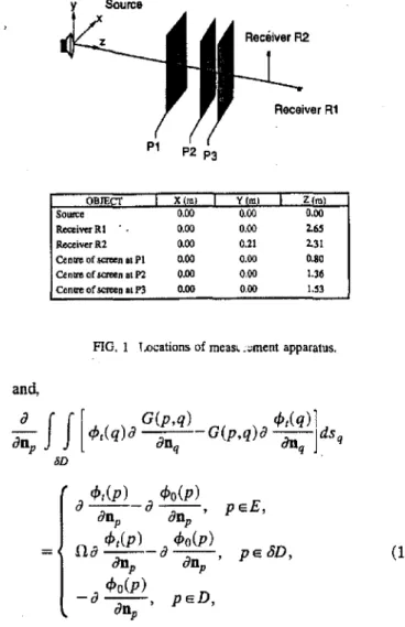
OBJEer X(m} I ytrn Zrn Source 0.00 0.00 a.GO R=1""rRI 0.00 a.oo 2.65 R=iverR2 0.00 0.21 2.31 CeOlre of saeenItPI 0,00 0.00 0.80 Centre or screen at P2 0.00 0,00 1.36 Cenn or screen8LP3 0.00 0,00 1.53 . iii'B :8-6

ｾ

4

ｾＲ

ｾｏｲＭＺ［ＭＺＮＬｾｾ］ＭＮＺＮＮＭＭＭＭＭＭＭＭＭＭＭｬ

51_2

c: --4 '---_-'---_-l..._--'_ _.l..-_..J-_-l...--J

o

FIG. 2. Comparison of approximate methods for determining the insertion loss of a singleO.4xOAm screen located atPI with the receiver atR1. The geometric calculation used the uniform theory of diffraction (Ref. 2).

FIG. 1 Locations of meas,Ｌｾｭ･ｮｴ apparatus.

10

r - - - ,

Souroe and, a

J

f[

G(p,q)

aD

p <Pr(q)

a aD

q 8D

a

eMp)

-a

4>o{p), pEE,

aD

_p

ao

p

=

oa

4>r(P)

-a

4>o(p) pE

aD,

(1b)

ao

_p

ao

_p ,

a

4>o(p) D

- --an-'

pE , p

where p is the point at which the velocity potential is to be solved,qthe point of integration, and

n

the ratio of the outer solid angle solid subtended at p to 4'IT. The total velocity potential <Pt is given by the sum of a scattered component <Ps and an unobstructed component ¢o;

The free-space Green's function is given by 1 eikjp-ql

G(p,q)=-4

-I-I'

(2b)

'IT p-q

where the wave number is defined as

52 J.Acoust. Soc. Am., Vol. 97. No.1, January 1995 T.R.T. Nightingale: Diffraction from two-dimensional objects 52

•

ｓｯｾｲ｣｡

•

RJaiver

(4b)

FIG. 4. Geometry for two-dimensional screensＨｳｵｲｦ｡｣･ｳｾＬ andｾｾ used in the discussion. .

method is used to predict the insertion loss due to multiple two-dimensional objects or screens of finite dimension. The predicted results are compared to the measured results and ｬＧｾ ｾ found to be in good agreement.

(4c)

I. EQUATION FORMULATION

For the purpose of development, we consider two per-fectly thin, flat and rigid screens as shown in' Fig. 4. The acoustic wave propagates from the point source located at

S

to the receiverR.The velocity potential on the rigid surface is given by

(4d)

(3a)

(4e)

where 8D

=

I

1+

I

_{2 •}The integration is performed over both

screen II and

I

2 , but each screen has two faces with

nor-mals differing in direction by7J'radians. Equation (3) repre·

sents a set of coupled simultaneous equations. Equation (3b) requires special treatment before it can be applied as it has a highly singular pole of the orderr-3in the domain of inte-gration. Terai3has shown that it can be replaced by the sum of three integrals. We focus our attention on Eq. (3a) as the introduction of approximate boundary conditions will allow us to use Eq.· (3a) alone to describe the surface potential, thereby removing the problems associated with the singular integrand of Eq. (3b).

Equation (3a) is expanded in terms of the surface poten-tials on each face (see Fig. 4):

where Pt is' the point at which velocity potential is to be determined on face Fl' and q1 the point of integration on

faceFIhaving normaln1 •Also, let the pointp lie inside the object and be the point to which the field points on opposite faces converge. The subscripts follow for the other faces. To decouple

Eq.

(4) which defines the surface potential, con-sider the following discussion.

Let the disturbance have a sufficiently small wavelength that the Kirchhoff boundary conditions are valid; that is, the disturbance on the "dark side" of each screen will be zero. This allows for the immediate simplification of

Eq.

(4) as now the surface potentials only need to be defined on a single face of each screen. Using the fact that the normal derivative of the free-space Green's function is zero when bothPandq are coplanar, we get

(Sa) (5b) 1

f

f

aG(p,q)

2'

tP,(p)-tPo(p)

=

q,t(q)

aO

q dsq , I, pe'!.2. ｱｅｾｬＧ 1

2'

q,/(p)-tPo(P) =0. (4a) (3b) pedD, which gives

Equation (6a) is simply twice the KBC for a point in an aperture (aperture 1) that is defined by a rigid screen. Equa-tion (6b) is the sum of an unobstructed component and a scattered component where the scattered component is the second RKl evaluated over the first screen. Using Babinet's principle (the unobstructed disturbance at a point p is the sum of the disturbances from the aperture. and a complemen-tary aperture that replaces the screen), Equation (6b) can be interpreted as beiog twice the field at a point in free space due to an aperture defined by screen1.The factors of 2 arise from the fact that we have constrained the point of observa-tion to lie on a screen surface. Due to the similarity to the KBC for an aperture and the RKls, Eq. (6) will be called the where we have dropped the subscripts for the integration and field points and the normals have heen taken to face away from the other screen.

Equations (5) represent a set of approximate coupled simultaneous equations. To decouple the set of simultaneous equations, consider the following geometrical discussion. Let the term "disturb;mce" mean velocity potential (<p); let

I,

define screen 1, and let

I,

define screen 2.As given by Eq. 2(a), the disturbance on

I,

will be the sum of components from the direct wave

cPo

and a scattered component<p, . Since

I,

is planar, there is no scattered component from points on

II [by Eqs. (3) and (Sa)]. However, II lloes e":,,,;ence a scattered componeot from

I,.

Employing geometrical con-cepts, the wave propagating from the source, as shown in Fig. 4, will have been diffracted 2n

+

1 times before it reaches

I"

where n is the multiple number (n=1...00).Again using an argument from the geometrical theories of diffrac-tion, the field is attenuated by approximately the wave num-ber (k)' after each diffraction by a large screen. Thus the scattered energy at the first screen which is due solely to a backscattered component from

I,

will be down by approxi-mately k(2n+l). Thus for moderate to high frequencies, the contribution due to multiples can be considered negligible, unless a low-order multiple facilitates a direct path to the receiver. By the same procedure, it can be argued that ifa scattered component on

Ii

is to be considered, it would be due solely to the component from

I,

and the effects of mul-tiple scattering should be ignored.

These arguments give the following boundary condi-tions and definicondi-tions of the surface potentials:

1

JJ

aG(p,q)

2

<p,(p) - <po(p)= <p,(q) an q ds q , I,

pE!",

qEI,.

(9) (8)

(7)

(lOa) a.G:...(:....a:.;.,b.:.,)d_A..::..b

2

-anb \<p,(a)\ 2aG(b,b )dA b <p,(b) 1----'--'-'-I anb aG(a,b) +2<p,(b) a dAb' nb

JJ

aG(a,b)

+

2 <p,(b) anb ds b, I, <p,(a)=2<po(a) . aG(b,a)

<p,(b)=2<Po(b) +2<p,(a)

an,

dA,

aG(b,b)

+2<p,(b) a dAb'

nb

JJ

aG(b,a)

<p,(b)=2<po(b)+2 <p,(a)

an,

ds,

I, =!2<Po(a)1 2<po(b) . 2_a:...:G:,..:(:.;.a,::.,a:.;.)d::.,A.:,'

1--an,

aG(b,a)dA, - 2

-'-'---'-=-an,

Thus far, no assumptions have been made about the ob-ject. However, if the object is planar then the second term of element (1,1) is zero, so too is that of element (2,2). Apply-ing the arguments used to formulate the MKBCs, the second term of element (1,2) is zero since we have assumed that

I

2

does not contribu.te to the field experienced atII'Expressing the remaining terms by their definite integrals gives

J J

.

aG(b,b)

+2 <p,(b) anb ds b.

I,

Equation (7) is discretized as if it were being numeri-cally integrated:

Collecting like terms and expressing them

in

a matrix form we get

J J

aG(a,a)

<p,(a)=2<Po(a)+2 <p,(a)

an,

ds,

II

aG(a,a)

<p,(a)=2<Po(a)+2<p,(a) a dA,

n,

modified Kirchhoff boundary conditions..

_,

An approximation of the total disturbance for an arbitrary point in space(pEE)

with an infinitely hard planar screen(s) present is given by applying the MKBCs to Eq. (la).

Itcan be shown that the method of MKBC decouples the

N byN set of equations of theｾｉ [Eq. (la)]. Let there be a single point of integration on each screen. There could be any number, but a single point is sufficient for illustration. Let point a be located on

It>

and point b on

I

2 . Equation (la) is therefore a set of 2 by 2 simultaneous equations as shown below: (6b) (6a) (5c)

[

PEI

_qEI;.

2 ,

JJ

aG(p,q) + <p,(q) an q dsq , I, and

(lOb)

or

(12a)

(l2b) The disturbance at a point in free space, given by

Eq.

(11), involves a quadruple integral (a surface integral of a surface integral) in addition to two surface integrals. Since there is generally no closed-form solution, numerical meth-ods must be employed, making the process very time con-suming. It would be highly desirable to reduce the surface integrals to a lower order, that is, a line integral around the rim of the aperture. Maggi and later Robinowitcz have stated that the

HKI

can be reduced to

a

line integral.I2 However, when a similar procedure is applied to the Rayleigh integrals, the method fails because a perfect differential can not be formed in the new coordinate system. Terai3used an image point source to construct a perfect differential. This has the effect of transforming the Rayleigh integral into the HKI.It has been shown13 that the HKIis just the mean of the first and second RKIs. Consequently, it can be shown that either of the RKIs can be replaced by the HKI without undue error when the two RKIs are approximately equal. This occurs when

III. EQUAnON SIMPUFICATION

(4)

It

_l and

I

₂coplanar: Since

II

and

I

2are coplanar, so too are the pointsp and q. Since the normal derivative of the

Green's function is zero for coplanar points, the last term in

Eq.

(6b) is zero. The remaining integrals can be expressed as a single surface integral over the screen.

(5)

II

and

I

₂ crossed: There exist a finite number of points along the line of intersection between

II

and

I

_{2 .} These points are contained in both

I

₁and

I

₂and are there-fore singular points in the domain of integration of Eq. (6b). The singularity only occurs whenp

=

qand can consequently be removed by using

Eq.

(6a) under these conditions.

(6) II_

oo:

The second term becomes minus the unob-structed and cancels with the first term. The expression

con-tained in the brackets of the last term becomes minus the unobstructed at the pointp on the second screen. The result

is no field at the observer.

(7)

I

2

-oo:

Invoking the reciprocity theorem of

Kirch-hoff, the last term becomes minus the second, thus canceling, while the first and third terms cancel. The result is no field at the observer.

The method of MKBC is based on the high-frequency approximation of the KBC. Consequently, we expect it to perform better in the high frequencies where the boundary conditions are more likely to be satisfied.As will be shown, the approximation is quite good, even whenthewavelength of the disturbance is similar to the object's dimension. For objects that are quite close together, the number of integra-tion points

will

have to be chosen such that the premise for numerical integration is valid (magnitude and phase approxi-mately constant across each integration area element). This might require a significant number of points for very small separations.

f

f

aG(b,a)

cP,(b)= 2cPo(b)

+

2 cP,(a) aDa dsb •

II

Thus the MKBCs decouple the Helmholtz integral equa-tions by using a high-frequency approximation based on the KBC for a single planar screen or aperture. Equation (lOa) is just twice the KBC. Equation (lOb) is twice the second RKI and can be thought of as being twice the disturbance that would have been.ｾｸｰ･ｲｩ･ｮ｣･､ in free spaceif a screen were placed between it and the source. The factors of 2 arise be-cause it is assumed that the pointp at which Eq. (10) is

evaluated lies on a surface and hence there is a mirror image present. The disturbance for a point in free space is given by applying the MKBCs to the HI. The expanded equation for an arbitraryｲ｣ｾｴ in space(R) exteriortothe objects(R eE)

is given by applying Eq. (6) to Eq. (ra), with the result:

ff

aG(s,q)

cPt(R)=</Jo(R)+2 cPo(q) aDI dSq

II

a.

nd

II. UMITlNG CONDITIONS

. aG(p,R) (11)

x

a

dsp '

D2

As expected from

Eq.

(2a), the total disturbance is the sum of an unobstructed component [the first term in Eq. (11)] and one or more scattered components (the remaining terms). The second and third terms of Eq. (11) are just the RKI describing the scattered components that would be experi-enced at the point of observation(R) if the screen(s) were apertures. The final term may be thought of

as

the scattered component from the second object due to a scattered com-ponent from the first (the term contained between the brack-ets).

+2

J

f

</Jo(P)

｡ｇ｡ｾｾｐＩ

dsp

12

Consider the result of

Eq.

(11) when the source and observer are on opposite sides of both

II

and

I

₂

as

shown in Fig. 2, under the following conditions:

(1) II-O: The effect of the first screen vanishes. The second term tends to zero so too does the fourth. The result-ing equation is just the RKI evaluated over

I

₂expressing the disturbance atR due to the presence of the screen

It

_{2 •}

(2)Ir-.O:The effect of the second screen vanishes. The third term tends to zero so too does the fourth. The resulting equation is just the RKI evaluated over II expressing the disturbance atR due to the presence of the

It!.

(3) II and

I

₂-O: It follows from the above that the second, third and fourth terms will tend to zero leaving just the unobstructed component.

where

Isqj

is approximately equal to the source-object

dis-ｴｾ｣･

and IqRI is approximately equal to the object-receiver distance for small objects. Thus when either Eqs. (12a) or 12(b) are satisfied for the appropriate boundary condition, the RKI can be replaced by the HKI and consequently the Maggi transform of the HKI. The Maggi transformation is given by

and where t is the tangent to the rim

r.

The boolean €is 1

when the line connecting the source and the point of obser-vation intersects the radiating surface; otherwise, it is zero. By comparing the results of the HKI and RKI shown in Fig. 2, it can be seen that for the objects and orientations consid-ered here, Eq.(12)is a good approximation. Substituting Eq.

(13) into Eq. (11) gives

cP(R)=lf.!o(R)O-€l+E2-€3)+-41

f

_al·tl

dl

'IT r₁

ep(p)

=

€cPo(p) -

Ｔｾ

Ir

a·t

dl,

where where

ro=qs,

rl

=qp, (13a) (13b) (13c)

IV. LIMITATIONS AND APPLICATIONS

The method presented provides a simple method for de-termining the disturbance due to multiple screens. While we have expressed the parameters of the problem in terms of multiple screens, it can also be interpreted in a more conven-tional way as being a problem involving multiple apertures-the aperture being defined as the screen's tended plane. The only limit of integration explicitly ex-pressed in terms of the screen is the last term of

Eq.

(14) as the others are expressed as contour integrals around the screen/aperture boundary.

The method presented is constrained by several limita-tions. First, the objects to be described must be constructed from finite two-dimensional planes as it was assumed that the normal derivative of the Green's function G(p,q) was zero. Second, the KBCs must be satisfied. This restricts the method to describe disturbances whose wavelength is much less than the object's dimension. Despite these limitations, the method is less restrictive than the geometrical methods. Even if the approximate boundary conditions are not satis-fied, the method still gives results that indicate the correct trend and in most cases the correct order of magnitude. This is quite unlike the geometrical method (UTD) of Fig. 2 which diverged rapidly when similar conditions were not met.

The application of the Maggi transformation to Eq. (11) introduces an additional constraint other than those given by Eq. (12). The transform fails if the point of observation lies on the edge of the geometrical shadow.!2 In that case, Eq.

(11)should be used rather than the simplified method.

I

V. RESULTS

Substituting the values given in Eq. (15) into Eq. (14) gives the following simple description for the cases consid-ered here:

For the screens and geometries considered here, the line be-tween the source and observation points always intersects the radiating surface, so

This section is broken into two parts. The first addresses the measurement systemand the physical properties it must have if the measurements and theoretical predictions are to be compared. In the final part, measured and predicted inser-tion losses are directly compared and the results discussed. A. Measurement system and basic requirements

The measurement system must reflect any explicit or implicit assumptions that were made during the formation of the MKBCs. These assumptions become requirements for the measurement system. They are

(1) source used must be a point source (Le., omnidirec-tional),

(2) KBCs must be satisfied for the screen(s) considered (this also implies that the transmission loss through the screen must be sufficiently high), and

(3) screens used must behave as if they were infinitely thin. Possible errors associated with these will be investigated in the sections following a description of the general mea-surement system.

1. General system

A convenient method for examining the accuracy of the theory is to compare the measured and predicted insertion loss due to a pair of screens. The measured insertion loss can be obtained by taking the ratio of the transfer functions (be-(15)

(14)

aG(R,p) (16)

a

.

dsp•

up

Having only two terms, a single and triple integral, Eq. (16) is much more compact. If the integration time ｶ｡ｲｩｾｳ directly with the number of integration points and there are

N points on each edge for line integrals and N2are used for the surface integrals, then Eq. (16) is 2N times faster to evaluate than Eq. (11).

i

45

1

ｾ

9

f

4 6 8 10 12 Frequency (kHz) Omni-Dlrectlonal Source •ｾ -ｾ • - - , 15

r---,

al10

:s.

ｾ

5 ﾧｏｾＧＢ］ＺＺＺ＾ＧＢＢ｡ｾｲ｟ＭＭＭＭＭＭＭＭＭＭｬ

:e

ｾ

-5 -10_'----l----l.-...J..-....l--..L---..t...J

o

2

FIG. 5. The effect on single screen insertion loss due to a directional source. OAXOAm screen located at PI with the receiver at R 1.

I + - - 60 ｾ

Ie 78

112

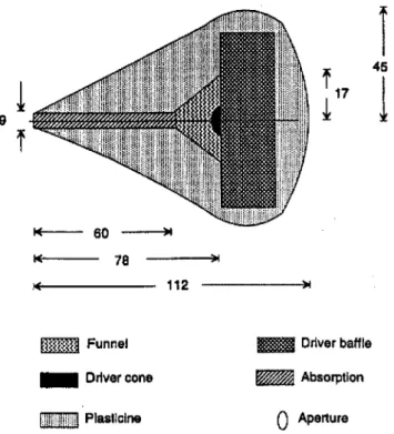
FIG. 6. Cross section of the constructed point source. Dimensions are in millimeters and are approximate.

tween the source excitation impulse and the microphone sig-nal) with and without It; ｾ｣ｲ･･ｮＨｳＩ in place. The predicted insertion loss is the ratio between the predicted sound-pressure level at the receiver with and without the screen(s) in place. The measurements were conducted in an anechoic chamber to minimize the effects of room reflections. Since no anechoic room is perfectly absorptive, time gating tech-niques were used to remove unwanted reflections. A high-pass filter set at

200

Hzwas used to remove low-frequency building noise.

mmm

Funnel _ Driver cone

HHi!!!!,!!!!!!1 Plasticine

l1li

Driver baffle

ｾ Absorption

o

Aperture

2. Source

In order to compare the measured results with the theo-retical predictions, which assume an ideal point source, it is necessary to construct a source that radiates energy equally in all radial directions. To illustrate this, the insertion loss for a OAXO.4 m screen at position PI and receiver position RI was measured using two different sources. The results are shown in Fig.5.The first, a highly directional source, was a Philips ADOI63 high-frequency driver having a cone diam-eter of about

2.5

em

mounted in

a

O.14XO.14XO.25 m ply-wood enclosure with sharp comers. The other, a much less directional source, used the same driver but the baffle effects were reduced by locating the O.75-cm-diameter radiating sur-face at the end of a long cylinder. Krishnappa14used a simi-lar method.

As shown in Fig. 6, the point source was constructed from a simple hard plastic funnel cut so its mouth was just wider than the driver's radiating surface. Steel wool was placed in the mouth in an effort to offer additional damping to the "driver's cone. Mineral wool was inserted in the throat to damp the standing waves that formed due to the mis-matched impedance between the funnel's throat and the air outside. The driver and funnel were then encased in a thick layer of plasticine to add mass in an effort to increase the transmission loss so the energy radiated by the sides was negligible relative to that from the aperture. The shape of the encasement was smooth and slowly varying, to remove any surface discontinuities. A sharp gradient in either the surface normal or its impedance becomes a line or point source as stated by Keller's geometrical theory of diffraction. Extend-ing the encasement to the back of the driver also improved its performance by creating a surface of homogeneous im-pedance. The amount of absorption in the funnel's throat was

chosen to attenuate the standing waves so that a sharp pulse could be emitted without undue smearing while maximizing the usable signal. If time gating techniques are to be used, then it. is very important to have a source that has a very short-tune constant so that the source does not continue to ring and emit energy after the pulse has arrived at the re-ceiver. Several different types of driving elements were tested. The type of element that had the longest ring was a piezoelement, followed by a voice coil of a hom driver as used by Krishnappa. Of the voice coil drivers, the KEF 1'27 had a shorter ring than the Phillips high-frequency driver but also had lower efficiency. Since there was a small path-length difference between the chamber floor and the bottom of the screen(s), the pulse duration had to be minimized. Thus the KEF driver was chosen. Alternatively, an inverse filter could have been used to create an excitation signal that, when emitted by the driver, would produce a near-delta func-tion.

A point source was created which radiated energy uni-formly to within ±O.75 dB over a solid angle of 11'/2 sr for an effective frequency range of 0.2-12.8 kHz. Comparing the results shown in Fig. 5 (with the object close to the source) to those shown in Fig. 7 (with the object further away), it can be seen that the effect of source directionality is reduced as the solid angle subtended from the source by the object is diminished.

3. Objects

The two-dimensional square screens were constructed from 19-mm plywood with square edges. Three different sizes were used: OAXO.4, O.5xO.5, and O.6xO.6 m, and could be located at the three positions shown in Fig. 1. The

12

r---,

-10

_m

Ｎｾ

:; 8

ＧＷＮＬＬＬＬＬＬｾＺｲ

.9 :

.'

l:

.2 2 19 mmSquare Edge Plywood -t:: Measurements 1 and 2 ｾｏｴＭＭＣＺＺＩ［ＺＺＺＺＺＭＭＭＭＧ［Ｇ［Ｇ［［［［Ｂ［［［ｾｾ［［［Ｂ［ＧＧＧＺＺＺＧＧＺＧ［ＺＧＧＺＺＧ｟ＭＭＭｪ .5 .2 -4Ｇ］ＢｏＭＭＺＲｾｾＴ ＭＭＺＶＭＭＸＺＭＭＭＱｾＰＭＭＭｊＱＲｾ Frequency (kHz) Omnl·Dlrectlonal Source \ I

.

,,,---

DIrectional Source

"

1 2 , - - - ,

....:10

a::I

_a

:E.

:ge

.94

52

1: (1)0ｲＭＭＭ［ＭＺ］ＭＭｾＧＭＭＭＭＭＭＭＭＭＭＭｬ I/) .£:-2 -4 0 l....>,.,l...2...&...,L-'-...l-....J...&.-.o....J,....,....L...>....J.".,.,..J...,...J-,...J 4

e

8 10 12 Frequency (kHz)

FIG. 7. The effect on single screen insertion loss due to a directional source. O.4XO.4 m screen located at P3 with the receiver at RI.

FIG. 9. Single screen insertion loss for O.SXO.5 m screens of various thick-nesses located at P3 with the receiver on axis at Rl. The two measurements of the 19·mm screen were made with different lime gates after the screen was removed and replaced toindicatemeasurement repeatability.

FIG. 8. Estimation of the field on the dark side of a single O.6xO.6 m screen at P3. The microphone positions are located very close to the screen's surface(10mm) to measure the sound pressure radiatedbythe dark side of the screen at the positions. This will provide insight to the validity of the KBCs for objects of this size.

not entirely satisfied in the region defined by the extended plane of the screen (Le., system's aperture) since the inser-tion loss is nonzero.

Figure 2 which compared measured and predicted inser-tion losses for a single screen shows that formulainser-tion based on the KBCs overestimated the insertion loss in the low fre-quencies but the agreement does improve with increasing frequency. This suggests that for source, object, and receiver positions considered here, theories that use the KBCs will

underestimate the sound-pressure level in the low frequen-cies. This may be explained by considering the KBC and MKBC assumption that there is no disturbance on the dark side of the screen(s).In reality, for wavelengths similar to the screen dimension there will most likely be a significant dis-turbance. Terai,3 when he performed an analytic determina· tion of the field on the dark side of a screen, found that even when the wavelength was about twice the object's dimension the disturbance on the

dark

side was comparable to that on the front. He also found that for source, object, and receiver configurations similar to those used here, the approximate KBC based method underestimated the receiver sound pres-sure.Itis possible that when the disturbance on the dark side is summed itwilltend to add in phase at the receiver, thereby reducing the insertion loss. Despite the fact the KBCs are not entirely satisfied

in

the low frequencies, the trend of the in· sertion loss curve is correctly predicted and the magnitude is usually accurate to within a few decibels for a single screen. The other assumption of the theoretical formulation is that the screen(s) can be considered as "thin" (i.e., one whose dimension approaches zero relative to the wave-length). The insertion loss of a 19-mm plywood screen was compared to that of a

3.2-mm

steel plate to determineif the plywood screens can be considered thin. The measured in-senion loss for 0.5 X0.5 m screen of various thicknesses is shown in Fig. 9. The results suggest that for frequencies up to about 8500 Hz the 19-mm-thick screen is behaving simi-larly to the much thinner 3.2·mm screen. For frequencies greater than 8500 Hz, the two screens exhibit different inser-tion losses with the difference apparently increasing with fre-quency. The plywood SCreen was removed and replaced and the measurement repeated with slightly different time gates to detennine if the observed difference was due to

measure-•

•

•

CI&p-Ia'Ctlment \Omm

--

•

.360rnm Offset .24D mmOff..t .12D mmOff",. ··li··· [0 mmOtlsal

f

300mm

1

60

r---,

$50 :2. 40 I/)

ＮＮｊ

ｾ 30 ,', c:20 " , . . A ... _ · ' ... •...v·

ｾ

10 ; . /...

·7·/· '-'

)60 mm Offset I/) ; ' 0) 240 mm Offset .E ｏｍｴＮＺＭＭＭＮＬＮＮ［ＮＮＮＮ［ＮＮ［ＮＬＮｾＺＮＮ［［ＮＮ［［［ＮＮＺＭＮＮＮＮＭＡＭ［［ＭＮＭＭＭＭＭｬ

., a

'="0ＭＭＺＲｾＭＭＢＧＭＭＮＮＮＮＮＮＮ｟ ...__.l...----'--.J 4 6 8 10 12 Frequency (kHz)

screens T""JISt satisfy several conditions if the predictions are to be accurately compared to the measured results.

The most basic requirement is that the screens should satisfy the KBCs upon which the MKBCs are built. This means that the disturbance on the dark side of the screen (Le., the side not facing the source) is negligible with respect to the disturbance on the side facing the sourCe. A further requirement is that the presence of the screen does not affect the field experienced in the extended plane of the screen (Le., the aperture). For wavelengths that are similar to the dimen-sions of the screen, the disturbance on the dark side of the screen does not satisfy the KBCs as shown by Fig. 8. If the KBCs were truly satisfied, then the insertion loss for all points immediately behind the screen but displaced a very small distance would be infinite for all frequencies. The fact that the insertion loss is not infinite will be due in part to the finite transmission ｬｯｾｳ of the plywood screen especially in the low frequencies. Also, Fig. 8 shows that the KBCs are

Calculated ----"",

.

\

,

\

I

Measured 4 6 8 10 12 Frequency (kHz) 40 - - - , mSO :2-ｾＲＰ

.9

510 1: Ql , ｾｏｪＮＮＺＮＮ［ＮＮＺＺＺＺ］ＺＮＭＭＭＭＭＭＭＭＭＭＭＮＮＮＮＮＬ .10 0 2 Difference 6 mm Square Edge PIY\'l'ood

ｾＬＧ｜

•

,.mm...

ｅｾＯＯ

4 0 , . . - . . . . - - - , al30

:2-ｾ

20

.9

510 t: Q)

.s

0

-10ＱＮＮＱＰＭＭＲＢＧＭＭＭＭＭＭＢＧＴＭＭＶＢＧＭＭｾＸＭＭＺＱＮＮＡＺＺＭｏＭＢＧＺＧＢＺＱＲｾ Frequency (kHz)

.

y- \

FIG. 10. Single screen insertion loss for O.SXO.S m screens of various tbicknesses located atP3 witb tbe receiver moved off-axis to R2. The

results indicate that effect of screen thickness on measured insertion loss is a function of source, screen, and receiver location.

FIG. 12, Insertion loss due to two screens O.6XO.6 m located at position Pi; O.6XO.6 m located at positionP2,with tbe receiver at Ri,N=12.

FIG. 11. Insertion loss due to two screens 0.4XO.4 m located at positionPl;

OAXO.4m located at positionP2.witb tbe receiver at Rl. The number of integration points on each edge,N, is varied to sbow tbe effect of under

sampling.

B. Comparison of measured and predicted results

Equation (16) waS used to compute the insertion loss for various systems. For the purposes of numerical integration, each edge was divided into 12 segments (N::::;12), giving a total of 48 segments for line integrals and 144· for surface integrals. The location. and the weighting of the integration points were determiited by Gauss-Legendre quadratures. The insertion loss was computed on a 386-based 25-MHz personal computer at discrete frequencies every 200 Hz over the measurement range 200-12800 Hz and took approxi-mately 90 s. Screen size, location, and point of observation are changed. The predictions are compared to measured re-sults and a method for determining the ninnber of integration points will be given. . .

Figure 11 shows the measured and predicted level change due to the system of screens (O,4XOA m at position

PI; 0.4XOA m at position

P2;

receiver position R 1). The

predicted results show ｴｾ･ correct trends in the frequency response of t.he inSertion loss, but the predicted results con-sistently overestimate the insertion loss. The overestimation can be as q1Uch as 3 dB. The predictions computed using three different numbers of integration points show that it is necessary to correctly choose the number of points as under-sampling will affect the high-frequency results. Figure 12 shows that increasing both screens' size to O.6XO.6 m does not affect the agreement. Inboth cases the model tends to overestimate

the

insertion loss in the low frequencies (i.e., when the wavelength is comparable to the object's dimen-sion). This is due to the higb·frequency approximation of the KBCs upon which the MKBCs are based.Aswas shownin

Fig. 2 (for a single screen), the KBCs and hence the MKBCs become a better approximation to the true field potential. on the dark side of a screen as the frequency increases. The fact that there are now two screens is likely to compound this error. Differences between measured and predicted results for frequencies greater than 8000 Hz may be due to the finite thickness of the screens. The thickness effects for a single screen, shown in Figs. 9 and 10, will be compounded since the system consists of two screens.

The method presented does not suffer from spurious re-sults at the eigenfrequencies of the space between the two objects as shown by the smooth continuous curves. For the

4 6 8 10 12 Frequency (kHz) 2 30 , . - - - , , Calculated

iil

25 J ' I

Ｌｾｎ］ＱＲ

a\"d 15 ｾＲＰ Ｌｾ l ...J

815

:\

ｾＧＮ｟ＧＭ

A ' ...

5

10 "...-- Calculated""";ｾ

i

5 " N = 6 (/) Measured

..501-==--1=---1

-5 0

ment repeatability. From the figure it can be seen that the difference due to thickness is greater than the uncertainty due to measurement repeatability. Thus the observed differences are due to the finite tbickness of the screens.

Figure 10 compares the measured insertion losses of a 19-mm and a 6-mm screen when the receiving point is moved off-axis. It can be seen that a significant difference between the two measured insertion 10ssg§ starts near 9500 Hz and the maximum difference is nearly 7 dB. This sug· gests that the effect of screen thickness on the measured insertion loss is both a function of frequency and the relative positions of the object and receiver. Despite this apparent uncertainty for very high frequencies, the 19-mm plywood screen exhibits similar insertion loss trends to screens of much lesser thickness. Thus 19-mm screens prove to behave like thin screens for most frequencies of interest, andin the very high frequencies they exhibit similar insertion loss trends to screens having much less thickness.

In the formulation of the MKBCs, and consequently Eqs. (11) and (16), it was assumed that the scattered compo-nent at

I

_{z was due solely to a component which had} under-gone a single diffraction (i.e., multiple diffractions between

I

1 and

I

z did not occur). Consequently, absorption was placed on the dark side of the screen nearest the source.

Calculated,',

\,'

I I I

,

20

r---....----,

iiJ 15

S

m

₁₀

oS

ｾ

5 Q.l

.s0h:-.I---l

-5 '-- t..--.-J_---'_--"_...J.._----'---l

o

2 4 6 8 10 12 Frequency (kHz) 5 0 , - - - , iiJ40 :5!. III30 III

..9

20 c:

ｾＱｏ

_Q.l

.s0l+---I

"10 , " - _ L - - _ L . - - _ " - - _ L . - - _ L . - - _ . J . . - . J

o

2 4 6 8 10 12 Frequency (kHz)

FIG. 13. Insertion loss due to two screens O.SXO.S m located at position

P1;O.SXO.S m located at positionP3,with the receiver atR2, N=12.

FIG.15. Insertion loss due to two screens O.6XO.6 m located at position

P1;0.4XO.4 m located at position P2, with the receiver atRl, N=12.

(17)

i

O.4m

1

ｾｾＭＭＭＭ .56m - - - l I t l l l

C.

Determining the number of Integration points

Selecting an adequate number of numerical integration points is critical to attaining a prediction that is not contami-nated in the high frequencies. Figure 11 has already shown the significant effect that using insufficient integration points can have on results. The number of points required will be a function of the frequency, the size of the screens, and the geometry between the source (either the point source or a field point on a screen) and the receptor points. Figure 16 shows two adjacent receptor points P1and P2 having

dis-tancesr1andr2to the field point$.Ingeneral, the follOWing

must hold:

ence, for the range

6-12.8

kHz, while for frequencies less than 6 kHz, the trend and details of the insertion loss are correctly represented by· the prediction which is within 3 dB of the measured.InFig. 15, the screens are interchanged and the degree of agreement remains similar. That is, the predic-tion tends to overestimate the inserpredic-tion loss. The differenceis typically less than 3 dB for frequencies below 6 kHz. For frequencies above 6 kHz both the trend and magnitude are correctly predicted. It is interesting to note that the level change during the first

4.

kHz is very similar.

12 10 2 4 6 8 Frequency (kHz) -. 30 , . . . - - - . . , iiJ25 '0 ";;'20 <Il

.s

15 Calculated,

ｾＱＰ

\ / Q) 5 Ｎｾｊ

..5

°

r:.:+---...:..---I

-50

case when SCreens are located at positions PI and P2, the fundamental ｦｲ･Ｌ｜ｵｾ｣ｹ is approximately 310

Hz.

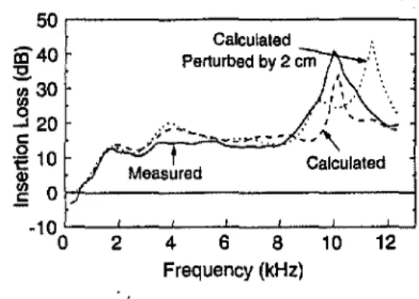
Figure 13 shows that the measured and predicted inser-tion losses for an off-axis point of observainser-tion (Le., receiver positionR2). For frequencies up to 9 kHz, the measured and predicted results agree within about 4 dB (with the prediction showing a higher insertion loss). After 9 kHz, the prediction only follows the general trend of the measured insertion loss. The difference between measured and computed may be due to the screens' finite thickness and also the uncertainty in the true relative positions of the source, screens, and receiver. Uncertainties in the object's position can significantly alter both the phase and magnitude of the predicted disturbance on the objects and ultimately the sound-pressure level at the receiver. To illustrate the sensitivity of the insertion loss on the screens' position, the computer model was run with the screens' position shifted by 2 cm in the positive

Y

direction. Figure 13 shows a significant insertion loss change for fre-quencies greater than 9000

Hz.

This effect should not be unexpected since shifting the screens by 2 em represents a change in position by more than X/2 at 9000

Hz.

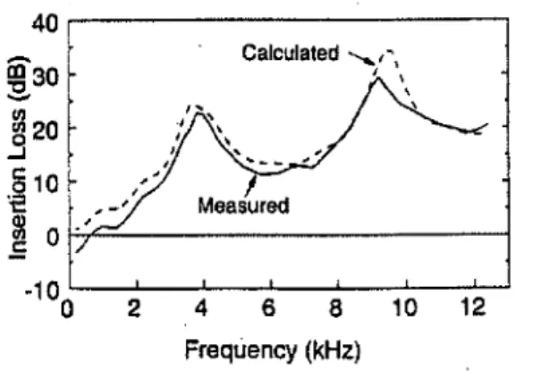
Ideally, detailed measurements made as a function of small pertUrba-tions would be used to evaluate this effect. However, such data are not available at the present time.

Thus far, only two screens of uniform size have been used. Now the case when the screens are of unequal size is considered. Figure 14 shows the result when there is a 0.4 XO.4 m screen at position PI and a O.6xO.6 m screen at positionP3.Agreement is very good, less than 2 dB

differ-FIG. 14. Insertion loss due to two screens OAXO.4 m located at position PI; O.6XO.6 m located at position P2, with the receiver at R I,N=12,

FIG. 16. Sketch showing integration points and the screen geometries used in determining the number of integration points for the O,4XOA m screens located at positions PI andP2 of Fig. 11.

t

t

i

_•

where 8 is some fraction of a wavelength. Ifthe Nyquist sampling theorem is applied, then

8= 'A/2.

If the angle be-tween the line'1and plane is 0,then Eq. (17)

can

be

rewrit-ten as

(ri+d 2sin2 O)1I2+d cos

O-'t=8=

Al2. (18)

Ideally, this would hold for all angles of 0 that are applicable to the system. For the geometry of the two screen system of Fig. 11, the range of angles is quite limited. The largest range occurring with the source on the first screen and the receptor points on theｳｾ｣ｯｮ､ screen is shown in Fig. 16. In this case, the range is approximately53°-90°. Figure 11 showed that with 6 points used for the line integrals and36 for the sur-face integrals, the error due to under sampling begins at about 6200

Hz.

Using the wavelength at 6200

Hz

(0.0553

m), Eq.. (18) suggests that there should be less than nine points on each edge (0=53") but more than ｴｨｲ･ｾ points (0

=90°). Using nine points on each edge would satisfy the condition [Eq. (18)] for the range of angles53°:S;;(}:!i;;90°but appears to be too conservative when the observed results of Fig. 11 indicated that only six points were required. How-ever, the mean of the two extremes (three points and nine points) represents a number which is in good 'agreement with the observed requirement of six points on each edge. This method requires further work to determine its applicability to more general geometries.

VI. CONCLUSIONS

The method of MKBC based on the KBCs has proved to be effective in predicting the surface potential on multiple two-dimensional objects. The MKBCs, when applied to the HIEM, decouple the N by N set of simultaneous equations. The resulting expressions for the surface potential can easily be integrated as there are no poles in the domain.

Experimentally the method was shown to offer a reason-able prediction of the disturbance at a pointinspace when there were two intervening screens. However, the method did suffer from the limitations associated with the KBCs upon whieh it is based. This was characterized by the method un" derestimating the sound-pressure level at the receiver in the low frequencies (hence an overestimation of the screens' in-sertion loss). Despite this, the correct inin-sertion loss trends were exhibited and the agreement tended to improve with frequency. Experimental work revealed that the 19-mm square edge screens used could not be considered "infinitely thin" for frequencies greater than about 8500

Hz

as the

thickness began to affect insertion loss. The effect of screen thickness was most pronounced for receiver positions off-. axis. The screens' finite thickness may have contributed to the deviation between measured and predicted results in the high frequencies. The insertion loss was shown to be greatly effected by shifts in position when distance Al2 or greater.

The MKBCs provide a convenient alternative, especially for objects and frequencies that are not well suited to either the geometrical theories of diffraction or the analytic meth-ods. The method of MKBC forms the basis for describing a special class of diffraction problems.

ACKNOWLEDGMENTS

The efforts of Professor Robert Craik, Heriot Watt Uni-versity, Scotland and the members of the Institute for Re-search in Construction, National ReRe-search Council Canada, especially those of Dr. John Bradley, are ｡｣ｫｮｯｷｬ･､ｧ･ｾＮＬ

IJ. Keller, "Geometrical theory of diffraction" J. Opl. Soc. Am. 52(2), 116-130 (1962).

2R. G. Kouyoumjian, and P. H. Pathak, "A uniform geometrical theory of diffraction for an edge in a perfectly conducting surface," Proc. IEEE 62, 1458-1461 (1974). .

3T. Terai, 1980, "On the calculation of sound fields around three dlmen-sional ,objects using integral equation methods," J. Sound. Vib. 69(1),

71-100 (1980). ..

4C. J. Bouwkamp, "Diffraction theory," Rep. Prog. Phys. 17, 35-72 (1954).

SA. Burton, "The solution of Helmholtz' equation in exterior domains

us-ing integral methods," National Physical Laboratory, NPL Rep. NAC 30 (1973).

6H. Schenck, "Improved integral formulation for acoustic radiation

prob-lems," J. Acoust. Soc. Am. 44(1), 41-58 (1968). .

7A. Seybert and T.Rengarajan, "The use of CHIEF10obtain solutions for

acoustic radiation using boundary integral equations," J. Acoust. Soc. Am. 81(5),1299-1306 (1987).

8A.Burton and G. Miller, "The application of internal equation methods to

the numerical solution of some exterior boundary value problems," Proc. R. Soc. London Ser A 323, 201-210 (1971).

9W. L. Meyer, W.A. Bell, and B. T. Zinn, "Boundary integral solutions of three dimensional acoustic radiation problems," J. Sound Vib. 59(2), 245-262 (1978).

10Z. Reut, "On the boundary integral methods for the exterior acoustic

problem," J. Sound Vib. 103, 297-298 (1985).

11K. Cunefare and G. Koopman, "A boundary element method for acoustic

radiation valid for all wave numbers," J.Accust. Soc. Am. 85(1), 39-48

(1989). .

12B. Baker and B. Copson, Huyge7lS' Principle (Clarendon, Oxford, 1950), pp.74.

13E. Wolf and E. Marchand, "Comparison of the Kirchhoff and the Rayleigh-Sommerfeld theories of diffraction at an aperture," J. Opt. Soc. AID. 54(5), 587-594 (1964).

14A.Krishnappa,USound intensity in the lIear field of a point source over a

hard reflecting plane," J. Acousl. Soc. Am. 81(2), 667-678 (1987).