Global glacier mass changes and their contributions
to sea-level rise from 1961 to 2016
M. Zemp1*, M. Huss2,3, E. Thibert4, N. Eckert4, R. McNabb5, J. Huber1, M. Barandun3, H. Machguth1,3, S. U. Nussbaumer1,3,
I. Gärtner-Roer1, L. Thomson6, F. Paul1, F. Maussion7, S. Kutuzov8 & J. G. Cogley9,10
Glaciers distinct from the Greenland and Antarctic ice sheets cover an area of approximately 706,000 square kilometres globally1, with
an estimated total volume of 170,000 cubic kilometres, or 0.4 metres of potential sea-level-rise equivalent2. Retreating and thinning
glaciers are icons of climate change3 and affect regional runoff4 as
well as global sea level5,6. In past reports from the Intergovernmental
Panel on Climate Change, estimates of changes in glacier mass were based on the multiplication of averaged or interpolated results from available observations of a few hundred glaciers by defined regional glacier areas7–10. For data-scarce regions, these results had
to be complemented with estimates based on satellite altimetry and gravimetry11. These past approaches were challenged by the small
number and heterogeneous spatiotemporal distribution of in situ measurement series and their often unknown ability to represent their respective mountain ranges, as well as by the spatial limitations of satellite altimetry (for which only point data are available) and gravimetry (with its coarse resolution). Here we use an extrapolation of glaciological and geodetic observations to show that glaciers contributed 27 ± 22 millimetres to global mean sea-level rise from 1961 to 2016. Regional specific-mass-change rates for 2006–2016 range from −0.1 metres to −1.2 metres of water equivalent per year, resulting in a global sea-level contribution of 335 ± 144 gigatonnes, or 0.92 ± 0.39 millimetres, per year. Although statistical uncertainty ranges overlap, our conclusions suggest that glacier mass loss may be larger than previously reported11. The present glacier mass loss is
equivalent to the sea-level contribution of the Greenland Ice Sheet12,
clearly exceeds the loss from the Antarctic Ice Sheet13, and accounts
for 25 to 30 per cent of the total observed sea-level rise14. Present
mass-loss rates indicate that glaciers could almost disappear in some mountain ranges in this century, while heavily glacierized regions will continue to contribute to sea-level rise beyond 2100.
Changes in glacier volume and mass are observed by geodetic and glaciological methods15. The glaciological method provides glacier-wide mass changes by using point measurements from seasonal or annual in situ campaigns, extrapolated to unmeasured regions of the glacier. The geodetic method determines glacier-wide volume changes by repeated mapping and differencing of glacier surface elevations from in situ, air-borne and spaceair-borne surveys, usually over multiyear to decadal periods. In this study, we used glaciological and geodetic data from the World Glacier Monitoring Service (WGMS)16, complemented by new and as-yet-unpublished geodetic assessments for glaciers in Africa, Alaska, the Caucasus, Central Asia, the Greenland periphery, Iceland, New Zealand, Scandinavia, Svalbard and the Russian Arctic. At present, this data set includes observations from 450 and 19,130 glaciers for the glaciological and the geodetic samples, respectively, which corre-spond to sample sizes of, respectively, less than 1% and 9% of the total number of glaciers1. We estimated regional mass changes for the 19 first-order regions of the Randolph Glacier Inventory (RGI)1 (Fig. 1).
The observational coverage ranges from less than 1% to 54% of the total glacier area per region for the glaciological sample, and from less than 1% to 79% for the geodetic sample (Extended Data Fig. 1). In each region, we combined the temporal variability from the glaciological sample—obtained using a spatiotemporal variance decomposition— with the glacier-specific values of the geodetic sample (see Methods). We then extrapolated the calibrated annual time series from the obser-vational to the full glacier sample to assess regional mass changes, taking into account regional rates of area change (see Methods). Uncertainties originate from four independent error sources. These relate to the temporal changes assessed from the glaciological sample, to the long-term geodetic values, to the extrapolation to unmeasured glaciers, and to estimates of regional glacier area. To estimate regional mass changes, we spatially interpolated the specific mass changes from the observational sample to all glaciers in the region. We estimated the related error from the deviations of this approach to regional (specific) mass changes, calculated as arithmetic averages or as area-weighted averages of the observational sample (see Methods).
Over the full observation period from 1961 to 2016, global glacier mass changes cumulated to −9,625 ± 7,975 Gt (1 Gt = 1012 kg). This
corresponds to a contribution of 27 ± 22 mm to global sea level, or a contribution of 0.5 ± 0.4 mm yr−1 when a linear rate is assumed. The total mass change excluding peripheral glaciers in Greenland and Antarctica sums to −8,305 ± 5,115 Gt, corresponding to a contribu-tion to sea level of 0.4 ± 0.3 mm yr−1. Cumulative mass changes and
corresponding contributions to global sea level were largest from the heavily glacierized regions, with approximately one third originating from Alaska (Fig. 1). Additionally, large contributions originate from regions with less glacierization but strongly negative specific mass changes, such as Western Canada and the USA (Extended Data Fig. 2). South Asia West was the only region that exhibited mass gain over the full observation period. Cumulative specific mass changes over this period, from 1961 to 2016, were most negative in the Southern Andes, followed by Alaska, the Low Latitudes, Western Canada and the USA, New Zealand, the Russian Arctic and Central Europe (Extended Data Fig. 2a). When annual rates are averaged over pentads (that is, periods of five years; Fig. 2), sea-level contributions ranged between 0.2 ± 0.5 mm yr−1 and 0.3 ± 0.4 mm yr−1 until the 1980s, and then increased continuously to reach 1.0 ± 0.4 mm in the lat-est pentad (2011–2016). Over corresponding periods, our lat-estimates show that global glacier mass loss is approximately equivalent to vari-ous mass-loss estimates from the Greenland Ice Sheet (between 2003 and 2012)12, and it exceeds present contributions to sea-level rise from the Antarctic Ice Sheet (2012–2017: 219 ± 43 Gt yr−1, including the Antarctic Peninsula)13 by 62%. Hence, glaciers contributed between 25% and 30% of the observed global mean sea-level rise, which ranged between 2.6 mm yr−1 and 2.9 ± 0.4 mm yr−1 over the satellite altimetry era (1993 to mid-2014)14.
1Department of Geography, University of Zurich, Zurich, Switzerland. 2Laboratory of Hydraulics, Hydrology and Glaciology (VAW), ETH Zurich, Zurich, Switzerland. 3Department of Geosciences,
University of Fribourg, Fribourg, Switzerland. 4Université Grenoble Alpes, Irstea, UR ETGR, Grenoble, France. 5Department of Geosciences, University of Oslo, Oslo, Norway. 6Department of
Geography and Planning, Queen’s University, Kingston, Ontario, Canada. 7Department of Atmospheric and Cryospheric Sciences, University of Innsbruck, Innsbruck, Austria. 8Department of
Glaciology, Institute of Geography, Russian Academy of Sciences, Moscow, Russia. 9Department of Geography, Trent University, Peterborough, Ontario, Canada. 10Deceased: J. G. Cogley.
*e-mail: [email protected]
http://doc.rero.ch
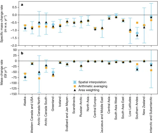
Glacier mass changes were negative in all regions over the latest observational decade, from 2006 to 2016 (Table 1)—that is, cov-ering the hydrological years15 from 2006/07 to 2015/16. Glaciers in South America had the most negative specific mass changes, with rates exceeding −1.0 m water equivalent (w.e.) per year, followed by glaciers in the Caucasus, Central Europe, Alaska, and Western Canada and the USA, with rates of less than −0.8 m w.e. yr−1 (Fig. 3a; 1 m w.e. = 1,000 kg m−2). The least negative specific mass changes were
found for glaciers in the Antarctic periphery (−0.1 m w.e. yr−1) and in South Asia West, with glaciers close to balanced-budget conditions17,18. Again, regions with large ice cover and negative specific mass changes showed the largest total losses (Fig. 3b). Record mass losses are thus found in Alaska, with rates of −73 Gt yr−1, followed by other heavily glacierized regions (that is, with glacier areas of more than 29,000 km2)
such as Arctic Canada North (−60 Gt yr−1), the Greenland periph-ery (−51 Gt yr−1), and the Southern Andes (−34 Gt yr−1; Table 1).
Exceptions are Central Asia and South Asia West, with limited mass losses (−7 Gt yr−1 and −1 Gt yr−1) despite their large glacier areas. Of the regions with smaller glacierization, Western Canada and the USA and Iceland lost the most mass, at rates of −12 Gt yr−1 and −8 Gt yr−1,
respectively.
We calculated the relative annual ice loss (Extended Data Fig. 3) by comparing present mass-change rates (2006–2016) with total esti-mated ice volumes for each region2. Nine out of nineteen regions lost between 0.5% and 3% of their total ice volume per year. The other regions featured smaller loss rates. Under present ice-loss rates, most of today’s glacier volume would thus vanish in the Caucasus, Central Europe, the Low Latitudes, Western Canada and the USA, and New Zealand in the second half of this century. However, the heavily gla-cierized regions would continue contributing to sea-level rise beyond this century, as glaciers in these regions would persist but continue to lose mass. It is worthwhile noting that a substantial part of the future ice loss is already committed owing to the imbalance of most glaciers with the present climate19,20, and that numerical models are required
to fully assess future glacier changes in view of climate-change scenarios20,21.
The total error bars related to regional mass changes (Fig. 3b) reflect a composite of different error sources. In most regions, the geodetic error accounts for the largest contribution, followed by the error related to temporal changes assessed from the glaciological sample (Extended Data Fig. 4). The extrapolation to unmeasured glaciers contributes substantially to the overall error only in regions with large differences between interpolation methods. The reasons for these differences are region specific and depend on various factors, such as the observational sample, the glacier size distribution, or a bias towards large tidewater or surge-type glaciers. Uncertainties related to glacier areas and their changes contribute only minimally to the overall error. However, con-sidering area changes is important despite their small contribution to random errors, as a constant glacier area over time would result in a systematic error that increases with the length of the time series and the rate of the area change22,23.
Our new approach, in combination with major advances in obser-vational evidence, allows for a sound assessment of global glacier mass changes independently of satellite altimetry and gravimetry. This is a basic requirement for the comparison of regional results and the detection of potential biases over the satellite era. By comparison with the Intergovernmental Panel on Climate Change’s Fifth Assessment Report (IPCC AR5)11,24, the greatest improvement herein is in the geodetic sample: it has been boosted from a few hundred glaciers7 to more than 19,000 globally, with an observational coverage exceeding 45% of the glacier area in 11 out of 19 regions (Extended Data Fig. 1). Our approach, combining the temporal variability from the glaciolog-ical sample with large-scale observations from the geodetic sample, facilitates the inference of mass changes at annual resolution for all regions, back to the hydrological year 1961/62. This represents a major development compared with IPCC AR511,24, which had to focus on the satellite altimetry and gravimetry era (2003–2009) and relied on estimates modelled using climate data or on interpolated values from
ACS WNA –416 Gt –428 Gt GRL –1,237 Gt TRP ISL SCA SAN –1,208 Gt ACN –1,069 Gt ASN CAU ASC NZL ASW ASE ANT CEU SJM RUA –687 Gt Global –1,044 Gt ALA –9,625 Gt –3,019 Gt
Cumulative mass change since 1961 (Gt) (362.5 Gt ≡ 1 mm s.l.e.) Specific mass-change rate (m w.e. yr–1)
> 0 0 to –0.25 –0.25 to –0.5 < –0.5 Glaciological sample Geodetic sample RGI glacier area
Fig. 1 | Regional glacier contributions to sea-level rise from 1961 to 2016. The cumulative regional and global mass changes (in Gt,
represented by the volume of the bubbles) are shown for the 19 first-order regions1 (outlined with bold black lines). Specific mass-change rates
(m w.e. yr−1) are indicated by the colours of the bubbles. In the background, the locations of glaciological and geodetic data samples are plotted over the glacier polygons from RGI 6.0. The grey plus signs mark latitudes and longitudes. As an example, glaciers in Alaska (ALA) show the largest contribution to sea-level rise, with a total mass change of approximately −3,000 Gt or 8 mm sea-level equivalent (s.l.e.) from 1961 to 2016, because
of a strongly negative specific mass-change rate (−0.6 m w.e. yr−1)
combined with a large regional glacier area. Note that South Asia West (ASW, blue bubble) is the only region in which glaciers slightly gained mass. ACN, Arctic Canada North; ACS, Arctic Canada South; ANT, Antarctic and Subantarctic; ASC, Central Asia; ASE, South Asia East; ASN, North Asia; CAU, Caucasus and Middle East; CEU, Central Europe; GRL, Greenland; ISL, Iceland; NZL, New Zealand; RUA, Russian Arctic; SAN, Southern Andes; SCA, Scandinavia; SJM, Svalbard and Jan Mayen; TRP, Low Latitudes; WNA, Western Canada and USA (see Table 1).
scarce and mostly uncalibrated observational samples for earlier time periods (see Methods).
Our central estimate for the global rate of glacier mass loss is 47 Gt yr−1 (or 18%) larger than that reported in IPCC AR5 (section 4.3.3.3, table 4.4)11,24 for the period 2003 to 2009 (Extended Data Fig. 5). A direct comparison of our results is possible for the seven regions (all with less than 15,000 km2 of ice cover) with estimates based on
glaci-ological and geodetic samples in IPCC AR511,24. In these regions, our mass-change estimates are systematically less negative (Extended Data Fig. 5a). This suggests that our new approach of calibrating regional glaciological mass-change time series with geodetic observations has overcome an earlier reported negative bias in the glaciological sample11. Regions with estimates based on satellite altimetry and gravimetry in IPCC AR511,24 featured absolute differences of the same order of mag-nitude but with varying signs. The more negative global mass changes result mainly from heavily glacierized regions where we estimate larger mass losses (for example, Alaska, peripheral Greenland and Antarctic, the Russian Arctic and Arctic Canada North), and are partly offset by smaller mass-loss estimates for a few other regions with abundant ice cover (for example, Arctic Canada South, Iceland, South Asia West, and Central Asia; Extended Data Fig. 5b) and by the above-mentioned bias in regions with less glacierization. Our error bars are considerably larger than and overlap with those reported in IPCC AR5 (section 4.3.3.3, table 4.4)11,24. However, a direct comparison is challenging, because the uncer-tainties in the earlier study11 were based on a combination of regionally different methods and data sources. A detailed comparison will require a regional assessment of glacier changes and related uncertainties, includ-ing scalinclud-ing issues from glacier-wide observations (this study) and results from satellite altimetry (regional averages of repeat-path measurements) and gravimetry (coarse resolution of sensor and hydrological models). However, our error estimates are methodologically consistent and con-sider all known relevant sources of potential errors. We concon-sider the relative differences of our error bars between the regions to be plausible and their absolute values to be upper bounds.
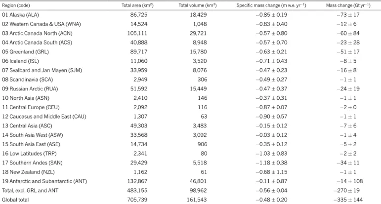
Improvements in global glacier mass-change assessments are still possible and necessary. First, the observational database needs to be extended in both space and time. We currently see the most urgent need for closing observational gaps being in regions where glaciers dominate runoff during warm/dry seasons, such as in the tropical Andes and in Table 1 | Annual rates of glacier change by region from 2006 to 2016
Region (code) Total area (km2) Total volume (km3) Specific mass change (m w.e. yr−1) Mass change (Gt yr−1)
01 Alaska (ALA) 86,725 18,429 −0.85 ± 0.19 −73 ± 17
02 Western Canada & USA (WNA) 14,524 1,048 −0.83 ± 0.40 −12 ± 6
03 Arctic Canada North (ACN) 105,111 29,721 −0.57 ± 0.80 −60 ± 84
04 Arctic Canada South (ACS) 40,888 8,948 −0.57 ± 0.70 −23 ± 28
05 Greenland (GRL) 89,717 15,780 −0.63 ± 0.21 −51 ± 17
06 Iceland (ISL) 11,060 3,520 −0.71 ± 0.43 −8 ± 5
07 Svalbard and Jan Mayen (SJM) 33,959 8,076 −0.47 ± 0.23 −16 ± 8
08 Scandinavia (SCA) 2,949 306 −0.49 ± 0.27 −1 ± 1
09 Russian Arctic (RUA) 51,592 15,449 −0.47 ± 0.37 −24 ± 19
10 North Asia (ASN) 2,410 146 −0.37 ± 0.31 −1 ± 1
11 Central Europe (CEU) 2,092 116 −0.87 ± 0.07 −2 ± 0
12 Caucasus and Middle East (CAU) 1,307 63 −0.90 ± 0.57 −1 ± 1
13 Central Asia (ASC) 49,303 3,483 −0.15 ± 0.12 −7 ± 6
14 South Asia West (ASW) 33,568 3,092 −0.03 ± 0.12 −1 ± 4
15 South Asia East (ASE) 14,734 906 −0.35 ± 0.12 −5 ± 2
16 Low Latitudes (TRP) 2,341 80 −1.03 ± 0.83 −2 ± 2
17 Southern Andes (SAN) 29,429 5,518 −1.18 ± 0.38 −34 ± 11
18 New Zealand (NZL) 1,162 61 −0.68 ± 1.15 −1 ± 1
19 Antarctic and Subantarctic (ANT) 132,867 46,801 −0.11 ± 0.87 −14 ± 108
Total, excl. GRL and ANT 483,155 98,962 −0.56 ± 0.04 −270 ± 19
Global total 705,739 161,543 −0.48 ± 0.20 −335 ± 144
The table shows present-day regional and global glacier areas and volumes, with specific mass changes (in m w.e. yr−1) and mass-change rates from spatial interpolation (in Gt yr−1) for the period from 2006 to 2016. Regional glacier areas are from RGI 6.0 and refer to the first decade of the twenty-first century1. Regional estimates for glacier volumes are based on ref. 2, updated to the glacier outlines
of RGI 6.0. Global totals are calculated as sums of regions for area, volume and mass change. Global specific mass changes are calculated by dividing the global mass-change rate by the global glacier area. Uncertainties correspond to 95% confidence intervals and originate from independent sources: glaciological sample, geodetic sample, spatial interpolation and glacier area (see Methods section ‘Uncertainty estimates’).
Fig. 2 | Global glacier contributions to sea-level rise from 1961 to 2016.
Annual and pentadal mass-change rates (left vertical axis) and equivalents of mean global sea-level rise (right vertical axis) are shown with related error bars (indicated by shading) corresponding to 95% confidence intervals. Annual errors originate from independent sources: glaciological sample, geodetic sample, spatial interpolation and glacier area. Over the five-year periods, the individual error terms are cumulated separately and then the multiyear terms are combined according to the law of random error propagations, and divided by the number of years (see Methods).
1960 1970 1980 1990 2000 2010 Year −600 −400 −200 0 200 400
Annual mass change
Annual change rate over 5 years
−1.0 −0.5 0.0 0.5 1.0 1.5 Sea-level equivalent (mm yr –1) Mass-change rate (Gt yr –1)
http://doc.rero.ch
Central Asia4, and in regions that dominate the glacier contribution to future sea-level rise, that is, Alaska, Arctic Canada, the Russian Arctic, and peripheral glaciers in Greenland and Antarctica. Second, a sys-tematic assessment of regional area-change rates25 will improve the estimate of corresponding impacts on regional mass changes. Finally, more research is required to better constrain the observational uncer-tainties at individual glaciers26 and for regional mass-change assess-ments. Despite these remaining challenges, our assessment of global glacier mass changes provides a new observational baseline for a sound comparison with estimates based on other methods27, as well as for future modelling studies of glacier contributions to regional runoff and global sea-level rise.
1. RGI Consortium Randolph Glacier Inventory (v.6.0): A Dataset of Global Glacier Outlines. Global Land Ice Measurements from Space, Boulder, Colorado USA
(RGI Technical Report, 2017) https://doi.org/10.7265/N5-RGI-60. 2. Huss, M. & Farinotti, D. Distributed ice thickness and volume of all glaciers
around the globe. J. Geophys. Res. 117, F04010 (2012).
3. Bojinski, S. et al. The concept of essential climate variables in support of climate research, applications, and policy. Bull. Am. Meteorol. Soc. 95, 1431–1443 (2014).
4. Huss, M. & Hock, R. Global-scale hydrological response to future glacier mass loss. Nat. Clim. Chang. 8, 135–140 (2018).
5. Marzeion, B., Cogley, J. G., Richter, K. & Parkes, D. Attribution of global glacier mass loss to anthropogenic and natural causes. Science 345, 919–921 (2014). 6. Radić, V. et al. Regional and global projections of twenty-first century glacier
mass changes in response to climate scenarios from global climate models.
Clim. Dyn. 42, 37–58 (2014).
7. Cogley, J. G. Geodetic and direct mass-balance measurements: comparison and joint analysis. Ann. Glaciol. 50, 96–100 (2009).
8. Kaser, G., Cogley, J. G., Dyurgerov, M. B., Meier, M. F. & Ohmura, A. Mass balance of glaciers and ice caps: consensus estimates for 1961–2004. Geophys. Res.
Lett. 33, L19501 (2006).
9. Dyurgerov, M. B. & Meier, M. F. Glaciers and the Changing Earth System: A 2004
Snapshot. Report INSTAAR/OP-58 (Instaar, 2005).
10. Ohmura, A. in The State of the Planet: Frontiers and Challenges in Geophysics Vol. 150 (eds Sparks, R. S. J. & Hawkesworth, C. J.) 239–257 (American Geophysical Union, 2004).
11. Gardner, A. S. et al. A reconciled estimate of glacier contributions to sea level rise: 2003 to 2009. Science 340, 852–857 (2013).
12. Khan, S. A. et al. Greenland ice sheet mass balance: a review. Rep. Prog. Phys.
78, 046801 (2015).
13. IMBIE. Mass balance of the Antarctic Ice Sheet from 1992 to 2017. Nature 558, 219–222 (2018).
14. Watson, C. S. et al. Unabated global mean sea-level rise over the satellite altimeter era. Nat. Clim. Chang. 5, 565–568 (2015).
15. Working Group on Mass-Balance Terminology and Methods of the International Association of Cryosphere Glossary of Glacier Mass Balance and Related Terms (UNESCO Digital Library, 2011) https://unesdoc.unesco.org/ark:/48223/ pf0000192525.
16. World Glacier Monitoring Service (WGMS) Global Glacier Change Bulletin No. 2
(2014–2015) (WGMS, 2017) https://doi.org/10.5904/wgms-fog-2017-10.
17. Brun, F., Berthier, E., Wagnon, P., Kääb, A. & Treichler, D. A spatially resolved estimate of High Mountain Asia glacier mass balances from 2000 to 2016.
Nat. Geosci. 10, 668–673 (2017); correction 11, 543 (2018).
18. Kääb, A., Treichler, D., Nuth, C. & Berthier, E. Contending estimates of 2003–2008 glacier mass balance over the Pamir–Karakoram–Himalaya.
Cryosphere 9, 557–564 (2015).
19. Mernild, S. H., Lipscomb, W. H., Bahr, D. B., Radić, V. & Zemp, M. Global glacier changes: a revised assessment of committed mass losses and sampling uncertainties. Cryosphere 7, 1565–1577 (2013).
20. Marzeion, B., Kaser, G., Maussion, F. & Champollion, N. Limited influence of climate change mitigation on short-term glacier mass loss. Nat. Clim. Chang. 8, 305–308 (2018).
21. Huss, M. & Hock, R. A new model for global glacier change and sea-level rise.
Front. Earth Sci. 3, https://doi.org/10.3389/feart.2015.00054 (2015).
22. Huss, M., Hock, R., Bauder, A. & Funk, M. Conventional versus reference-surface mass balance. J. Glaciol. 58, 278–286 (2012).
23. Paul, F. The influence of changes in glacier extent and surface elevation on modeled mass balance. Cryosphere 4, 569–581 (2010).
Fig. 3 | Regional estimates of glacier mass change for the period 2006–2016. a, b, Annual mass-change rates in metres of water equivalent
per year (a) and in gigatonnes per year (b) as estimated from spatial interpolation (blue circles), area-weighting (black triangles) and arithmetic averaging (orange squares). The spatial-interpolation approach is the reference, with results provided in Table 1. Error bars correspond
to 95% confidence intervals, and consider uncertainties related to the temporal variability of the glaciological sample, the geodetic value, the regional interpolation, the regional glacier area, and a second-order crossed term. We estimate the error related to the regional interpolation from the differences between the three interpolation approaches (see Methods section ‘Uncertainty estimates’).
–2.0 –1.5 –1.0 –0.5 0.0 0.5 a Alaska
Western Canada and USA
Arctic Canada North Arctic Canada South
Greenland
Iceland
Svalbard and Jan Mayen
Scandinavia
Russian Arctic
North Asia
Central Europe
Caucasus and Middle East
Central Asia
South Asia West South Asia East
Low Latitudes
Southern Andes
New Zealand
Antarctic and Subantarctic
–150 –125 –100 –75 –50 –25 0 25 50 b Spatial interpolation Arithmetic averaging Area weighting Mass-change rate (Gt yr –1)
Specific mass-change rate
(m w.e. yr
–1
)
24. Vaughan, D. G. et al. in Climate Change 2013: The Physical Science Basis.
Contribution of Working Group I to the Fifth Assessment Report of the Intergovernmental Panel on Climate Change (IPCC) (eds Stocker, T. F. et al.)
317–382 (Cambridge Univ. Press, Cambridge, 2013).
25. Cogley, J. G. Glacier shrinkage across High Mountain Asia. Ann. Glaciol. 57, 41–49 (2016).
26. Zemp, M. et al. Reanalysing glacier mass balance measurement series.
Cryosphere 7, 1227–1245 (2013).
27. Marzeion, B., Leclercq, P. W., Cogley, J. G. & Jarosch, A. H. Global reconstructions of glacier mass change during the 20th century are consistent. Cryosphere 9, 2399–2404 (2015).
Acknowledgements We thank the national correspondents and principal
investigators of the WGMS network as well as the Global Land Ice
Measurements from Space (GLIMS) and RGI communities for free and open access to their data sets. We thank B. Armstrong for polishing the language. Arctic digital elevation model (DEM) strips were provided by the Polar Geospatial Center under National Science Foundation (NSF) Office of Polar Programs (OPP) awards 1043681, 1559691 and 1542736. This study was enabled by support from the Federal Office of Meteorology and Climatology MeteoSwiss within the framework of the Global Climate Observing System (GCOS) Switzerland, the Cryospheric Commission of the Swiss Academy of Science, the Copernicus Climate Change Service (C3S) implemented by the European Centre for Medium-range Weather Forecasts (ECMWF) on behalf of the European Commission, the European Space Agency (ESA) projects Glaciers_cci (4000109873/14/I-NB) and Sea-Level Budget Closure CCI (4000119910/17/I-NB), and Irstea Grenoble as part of LabEx OSUG@2020.
Reviewer information Nature thanks A. Rowan and the other anonymous
reviewer(s) for their contribution to the peer review of this work.
Author contributions M.Z. initiated and coordinated the study and wrote
the manuscript; the basic concept was jointly developed during a workshop in the Swiss pre-Alps. J.G.C. compiled extensive data from the research community and the literature, and was a dedicated glaciologist and pioneer in glacier mass-balance studies. M.Z., S.U.N., H.M., I.G.-R., J.H., F.P., L.T. and S.K. compiled data from the research community and the literature. R.M., J.H. and M.B. computed additional geodetic results. M.H., M.B. and F.M. defined clusters and regions used in the analysis. E.T. and N.E. ran the variance decomposition model. M.H. performed the calibration of the glaciological signal to the geodetic series and the extrapolation to regional changes. M.Z., I.G.-R., S.U.N., E.T. and J.H. produced the figures. All authors commented on the manuscript.
Competing interests The authors declare no competing interests.
Additional information
Extended data is available for this paper at https://doi.org/10.1038/s41586-019-1071-0.
Reprints and permissions information is available at http://www.nature.com/ reprints.
Correspondence and requests for materials should be addressed to M.Z. Publisher’s note: Springer Nature remains neutral with regard to jurisdictional
claims in published maps and institutional affiliations.
© The Author(s), under exclusive licence to Springer Nature Limited 2019
METHODS
Glaciological and geodetic mass changes. The glaciological method usually
provides glacier-wide surface mass balance (Bsfc) over an annual period related
to the hydrological year. In line with ref. 15, we use the unit m w.e. for the
spe-cific mass change (1 m w.e. = 1,000 kg m−2) and the unit Gt for the mass change
(1 Gt = 1012 kg), with mass balance and mass change as synonymous terms. Results
are reported as cumulative values over a period of record or as annual change rates (yr−1). The geodetic balance is the result of surface (sfc), internal (int) and basal (bas) mass changes and—in the case of marine-terminating or lacustrine glaciers—of calving (D) in the unit m w.e.:
= Δ = + + +
Bgeod M Bsfc Bint Bbas D
In practice, the geodetic (specific) mass change is calculated as the volume change, ΔV, over a survey period between t0 and t1, from differencing of DEMs, over the
glacier area multiplied by a volume-to-mass conversion factor:
ρ ρ = Δ × − × B V S t t 1 ( ) geod 1 0 water
where S is the average glacier area of the two survey times (t0, t1) assuming a linear
change through time26, and ρ is the average density of ΔV with a commonly
applied value28 of 850 ± 60 kg m−3. The glaciological method is able to
satisfacto-rily capture the temporal variability of the glacier mass change even with only a small observational sample29,30. However, its cumulative amount over a given time
span is sensitive to systematic errors, which accumulate with the number of annual measurements31,32. The geodetic method provides mass changes covering the entire
glacier area and large glacier samples. However, the method requires a density conversion and surveys are typically carried out at multi-annual to decadal inter-vals only. For both measurements, we use the latest version (wgms-fog-2018-06) of the Fluctuations of Glaciers (FoG) database from the WGMS16. The
glaciolog-ical sample was recently updated with observations from latest years, consolidated by adding results from approximately 100 additional glaciers7, and the entire
mass-balance series was replaced after reanalysis33–37. The geodetic sample was
increased recently by the inclusion of large-scale assessments from several moun-tain regions17,38–42.
For the present study, we complemented the dataset from the WGMS with an additional 70,873 geodetic volume change observations computed for 6,551 glaciers in Africa, Alaska, the Caucasus, Central Asia, Greenland’s periphery, Iceland, New Zealand, the Russian Arctic, Scandinavia and Svalbard (Extended Data Table 1). This was achieved by calculating geodetic mass changes from ASTER DEMs processed using MMASTER43 which were co-registered using
off-glacier elevations from the Ice, Cloud, and land Elevation Satellite (ICESat) as common frame following ref. 44. Where available, we used ArcticDEM 2-m
strips, SPOT5-based DEMs from IPY-SPIRIT or the High Mountain Asia 8-m DEMs45 to increase spatial and temporal coverage, after resampling to 30-m
res-olution to match the resres-olution of the ASTER DEMs. Pairs of DEMs (for example, ASTER/ASTER or ASTER/ArcticDEM) were automatically chosen on the basis of at least 40% overlap and a time separation of at least eight years. This time separation, together with the selection of DEMs towards the end of the ablation period (Extended Data Table 1), aimed to reduce the effect of seasonal variations in the surface elevation and minimizes differences to glaciological survey dates. On the basis of the selected DEM pairs, glacier elevation changes were computed for various time periods between 2000 and 2018. We used the local hypsometric method46 to fill voids in the DEMs. For each glacier outline with an area of at
least 0.6 km2 from RGI 6.0, we calculated the glacier hypsometry using 100-m
elevation bins. For each DEM pair, we calculated the mean elevation difference per elevation bin, and multiplied this by the glacier hypsometry to obtain a volume change. The longest available differences with at least 70% data coverage were then used for each glacier to obtain the geodetic mass change. For the peripheral glaciers in Western Greenland, geodetic mass changes were calculated using the Aero DEM47 from 1985 and a prerelease of the 2010–14 TanDEM-X Global DEM.
Before differencing, all DEMs were co-registered to each other44. We estimated
the glacier volume change with the local hypsometric method46, using elevations
derived from TanDEM-X and the RGI 6.0 outlines. Again, only glaciers with at least 70% data coverage were used. We estimated uncertainties in geodetic mass changes on the basis of off-glacier differences between the two DEMs after co-registration, following the approach of ref. 17.
Glacier inventory. We derived the global distribution of glaciers from the
RGI1,48, which is a snapshot glacier inventory derived from the Global Land Ice
Measurements from Space (GLIMS) database49 and a large compilation of national
and regional sources compiled by the RGI consortium1. We used glacier area and
its distribution with elevation (that is, glacier hypsometry) for the 215,547 glaciers in RGI 6.0, covering a total area of 705,739 km2, mainly for survey years between
2000 and 2010. Improvements with respect to earlier RGI versions as used in IPCC
AR511,24 (168,331 glaciers, 726,258 km2) include the separation of glacier
com-plexes (for example, ice fields or ice caps) into individual glaciers, replacement of nominal glaciers (that is, size-equivalent circles) by real glacier outlines, assignment of glacier-specific survey dates, and the introduction of glacier-specific hypso-metries (Extended Data Fig. 1). The latter come as a list of elevation-band areas (at a resolution of 50 m in height) in the form of integer thousands of the glacier’s total area1. Note that at present the RGI includes peripheral glaciers surrounding the
Greenland Ice Sheet50 but not the peripheral glaciers on the Antarctic Peninsula51
and in the McMurdo Dry Valleys52. For future versions of the RGI, the inclusion
of these peripheral glaciers in Antarctica should be considered in order to reach global completeness and consistency with the classification of peripheral glaciers in Greenland50.
Changes in glacier area. For hydrological and sea-level applications, it is the
con-ventional mass balance that is relevant—that is, the mass change calculated over a constantly changing area and hypsometry of a glacier15. While the changes in
hypsometry are implicitly captured, the changes in glacier area need to be explicitly accounted for by both the glaciological and the geodetic methods26. In contrast
with earlier approaches, we considered the impact of changes in glacier area over time on regional mass-change estimates. Therefore, we used a collection of relative area changes from IPCC AR5 (chapter 4, figure 4.10 and table 4.SM.1 of ref. 24),
extended with additional literature53–55 to obtain area change rates for all first-order
glacier regions.
Glacier volume estimates. Regional estimates for glacier volumes are based on
ref. 2, updated to the glacier outlines of RGI 6.0.
Spatial regionalization. For regional analysis, it is convenient to group glaciers
by proximity. We achieved this by using the latest version of glacier regions as available from the Global Terrestrial Network for Glaciers56. These 19 first-order
and more than 90 second-order regions derive ultimately from glacier regions proposed by the GLIMS project around the year 2000 and from studies dealing with global glacier distribution57,58, and are implemented in both the RGI and the
FoG databases. For mass-balance studies, the 19 first-order regions seem to be appropriate because of their manageable number and their geographical extent, which is close to the spatial correlation distance of glacier mass-balance variability (that is, several hundred kilometres)59,60. We further divided these regions for areas
that are known to feature large diversities in mass-balance gradients and where sufficient data coverage allowed (Extended Data Table 2).
Extraction of temporal variability from the glaciological sample. In a first step,
we subdivided the sample of glaciological series into spatial clusters. We started from the smallest possible units (second-order glacier regions) and then extended them until the number and completeness of the time series was acceptable to ensure a proper variance decomposition based on visual and quantitative criteria, such as a common mass-balance temporal variability (that is, a high correlation between annual mass-balance series) and spatial consistency (that is, a cluster cannot be geographically too wide). The resulting 20 regional clusters correspond to first- and second-order glacier regions or a combination thereof (Extended Data Table 2). For half of these clusters, the available mass-balance series cover the full survey period with only minor data gaps of a few years. For the other half of the clusters, we com-plemented the glaciological sample with a few long-term series from neighbouring regions that feature a similar mass-balance variability (Extended Data Table 2). For the few clusters without glaciological data before the mid-1970s, we used the mean value of the geodetic sample (that is, neglecting interannual variability) for these years and set the related uncertainty to twice the average value of the first decade with glaciological observations.
In the second step, we extracted the temporal mass-balance variability for each cluster using a variance decomposition model61, which is a further development of
the approach of ref. 30, based on Bayesian techniques62,63 and applied to a regional
sample of glacier-wide mass balances instead of to a series of point measurements. For this model, we defined the specific mass change for a given glacier i and year
t as:
α α ε
= + + + +
Bglac, ,i t 0 i g t( ) z t( ) i t, (1)
where α0 is the cluster’s annual average and αi is the glacier-specific site devia-tion of the (specific) mass change from the cluster’s average. The variables g(t) and z(t) are the long-term trend and annual fluctuations, respectively, of the time deviation from the average, and εi,t are residuals. The variable g(t) was taken as a smooth nonparametric trend and z(t) as a white-noise term. Their sum is the annual deviation of the glaciological sample from the average α0, which is further used in the analysis:
= +
Bglac,cluster g t( ) z t( ) (2)
Model inference was performed using Bayesian simulation techniques, giving access, for any parameter or combination of parameters, to a point estimate and to a credibility interval quantifying the related uncertainty. This especially applies to
cumulated temporal deviations ∑tt t=2 1( ( )g t +z t( )) over any time interval [t1,t2],
such as the full period from 1961 to 2016 (Extended Data Fig. 6)
Calibration to mass-change values from the geodetic sample. For each cluster
(Extended Data Table 2), we calibrated the temporal mass-balance variability as derived from the glaciological sample Bglac,cluster to the values from the geodetic
methods26. Owing to the differences in length of the geodetic survey periods, we
carried out the calibration individually for all glaciers with available geodetic bal-ances. If more than one geodetic survey was available per glacier, we combined those with the longest survey periods by arithmetic averaging of annual change rates. For each glacier i, we calculated the mean annual deviation βt between the glaciological balance of the cluster Bglac,cluster and the glacier-specific geodetic
bal-ance Bgeod,i over a common time period of N years between t0 and t1:
β =t Bgeod,i− ∑NtBglac,cluster (3)
t
o
1
The annual calibrated specific mass change for every glacier i and year t was then calculated as:
β
ΔMcal, ,i t=Bglac,cluster,t+ t (4)
As a result, for each glacier with available geodetic data we obtained a calibrated specific mass-change series that features the temporal variability of the glaciological cluster but is adjusted to the glacier-specific geodetic value (Extended Data Fig. 7).
Regional mass changes and contributions to sea level. To estimate the total mass
change, we need to scale the results from the sample with available (geodetic) data to all glaciers of a region (from RGI 6.0). We followed three different approaches to calculate the regional specific mass change ΔMregion (in units of m w.e. yr−1):
arith-metic averaging ΔMregion,AVG, area-weighting ΔMregion,AW, and spatial interpolation
ΔMregion,INT. For the approaches ΔMregion,AVG and ΔMregion,AW, we assigned the
arithmetic and glacier area-weighted average, respectively, of the annual specific mass change of the observational sample to all unobserved glaciers in the region. For our reference approach ΔMregion,INT, we spatially interpolated the individual
specific mass-changes to all glacier locations in the region using an inverse distance weighting function. For all approaches, we calculated the regional mass change ΔMregion (in units of Gt yr−1) as the product of the specific mass change multiplied
by the regional glacier area from RGI 6.0, applying the relative area change rates of the corresponding region. Global mass changes, ΔMglobal, were calculated as
the sum of all regional mass changes. For conversion to sea-level equivalent, we assumed a total area of the ocean of 362.5 × 10⁶ km2 (ref. 64).
Uncertainty estimates. The random error of the regional mass change, σregional, is composed of the errors related to: first, the temporal changes in the regional glaciological sample σglac; second, the geodetic values of the individual glaciers
σgeod; third, the extrapolation from the observational to the full sample σextrapolation; fourth, the glacierized area σarea of the region; and fifth, a second-order crossed term related to the calculation of the regional mass change (as the product of specific mass change multiplied by the glacierized area):
σregional= σglac+σ +σ +σ +σ (5) 2 geod 2 extrapolation 2 area 2 crossed 2
The variable σglac can be rigorously estimated from the variance decomposi-tion (Extended Data Fig. 6). However, we used a less computadecomposi-tionally intensive approach to estimate it for any subperiod (pentad, decade) from the full study period. Specifically, the annual standard deviations of the temporal deviation (g(t) + z(t)) as obtained from the variance decomposition model were summed up according to the law of random error propagation. Hence, the standard deviation of any subperiod was evaluated as if annual deviations would be independent. The variable σglac implicitly accounts for errors related to differences in the glaciological survey period, because the sample contains results from various time systems (for example, fixed-date, floating-date and stratigraphic)15.
The variable σgeod is the uncertainty from the geodetic method. We calculated the annual values as rates—that is, dividing the reported (multiyear) uncertain-ties by the number of years between the two surveys. It includes the observation uncertainty σgeod.observation as reported with the geodetic results. In addition, we considered the uncertainty introduced by calibrating annual mass-balance varia-bility with geodetic values, σcalibration (Equation (4)), which was inferred for each glacier individually on the basis of randomly superimposing σglac and extracting the standard deviation of average balances over the reference period. The uncertainties related to density conversion factor σdensity were set to ± 60 kg m−3 according to
ref. 28. The overall geodetic uncertainty was calculated from these terms, assuming
them to be uncorrelated, and was divided by the square root of the number of independent items n of information in the sample:
σgeod= σ . +σn +σ
geod observation2 calibration2 density2
In the ideal case, n would be equal to the number of geodetic series in the regional sample. For spaceborne surveys, however, the geodetic uncertainty is usually derived from the stable terrain in between a group of glaciers. We thus assumed geodetic uncertainties uncorrelated for samples larger than 50 glaciers, and esti-mated n by dividing the regional geodetic sample size by 50. Note that, for the geodetic sample, we do not explicitly formulate uncertainties related to differences in the survey date. For individual glaciers, a corresponding rigorous estimate would be possible using seasonal mass-balance information, meteorological data, and numerical modelling7,26,33. These studies show that the corresponding
uncertain-ties can be relevant for individual years but tend towards zero for longer periods of records and larger samples.
To estimate σextrapolation, we used the regional mass change from spatial interpo-lation (ΔMregion,INT) as a best guess and calculated the extrapolation uncertainty
as 1.96 standard deviations of the results from the three approaches (ΔMregion,INT,
ΔMregion,AVG and ΔMregion,AW). As for σglac, we evaluated σextrapolation over any
sub-period by the square root of the number of survey years, assuming that annual values are uncorrelated.
For the regional glacier area, we assumed a general uncertainty of ± 5% for the total area derived from RGI 6.0, given earlier single-glacier and basin-scale uncer-tainty estimates48 and in line with the latest GCOS product requirements (table 25
of ref. 65; terrestrial essential climate variable (ECV) product requirements). This
uncertainty was combined with an error related to the regional area changes
σarea.change, which was estimated as 1.96 standard deviations of the different approaches used to calculate regional change rates. For a given region, the first approach, used as reference, weights multiple published change rates by the total ice cover of the corresponding glacier samples. The second approach weights multiple results by the length of the survey periods. The uncertainties related to the total area and to area changes were assumed to be uncorrelated and, hence, cumulated according to the law of random error propagation.
Over multiyear periods, in contrast with σglac, σextrapolation and σcrossed, the errors related to the geodetic values and glacier areas (σgeod and σarea) cumulate linearly. Consequently, the individual terms need to be cumulated separately, followed by a combination of the multiyear terms according to the law of random error prop-agation (see equation (5)). For global sums, the overall error was calculated by cumulating the regional errors according to the law of random error propagation.
Data availability
The temporal variabilities for the glaciological clusters as well as the regional and global mass-change results have been deposited in the Zenodo repository (https:// doi.org/10.5281/zenodo.1492141). The full sample of glaciological and geodetic observations for individual glaciers is publicly available from the WGMS (https:// doi.org/10.5904/wgms-fog-2018-11).
Code availability
The analytical scripts are available from the authors on request.
28. Huss, M. Density assumptions for converting geodetic glacier volume change to mass change. Cryosphere 7, 877–887 (2013).
29. Fountain, A. G. & Vecchia, A. How many stakes are required to measure the mass balance of a glacier? Geogr. Ann. Ser. A 81, 563–573 (1999).
30. Lliboutry, L. Multivariate statistical analysis of glacier annual balances. J. Glaciol.
13, 371–392 (1974).
31. Cox, L. H. & March, R. S. Comparison of geodetic and glaciological mass-balance techniques, Gulkana Glacier, Alaska, U.S.A. J. Glaciol. 50, 363–370 (2004). 32. Thibert, E., Blanc, R., Vincent, C. & Eckert, N. Glaciological and volumetric mass-balance measurements: error analysis over 51 years for Glacier de Sarennes, French Alps. J. Glaciol. 54, 522–532 (2008).
33. Huss, M., Bauder, A. & Funk, M. Homogenization of long-term mass-balance time series. Ann. Glaciol. 50, 198–206 (2009).
34. Andreassen, L. M., Elvehøy, H., Kjøllmoen, B. & Engeset, R. V. Reanalysis of long-term series of glaciological and geodetic mass balance for 10 Norwegian glaciers. Cryosphere 10, 535–552 (2016).
35. Thomson, L. I., Zemp, M., Copland, L., Cogley, J. G. & Ecclestone, M. A. Comparison of geodetic and glaciological mass budgets for White Glacier, Axel Heiberg Island, Canada. J. Glaciol. 63, 55–66 (2016).
36. Wang, P., Li, Z., Li, H., Wang, W. & Yao, H. Comparison of glaciological and geodetic mass balance at Urumqi Glacier No. 1, Tian Shan, Central Asia. Global
Planet. Change 114, 14–22 (2014).
37. Basantes-Serrano, R. et al. Slight mass loss revealed by reanalyzing glacier mass-balance observations on Glaciar Antisana 15α (inner tropics) during the 1995–2012 period. J. Glaciol. 62, 124–136 (2016).
38. Fischer, M., Huss, M. & Hoelzle, M. Surface elevation and mass changes of all Swiss glaciers 1980–2010. Cryosphere 9, 525–540 (2015).
39. Vijay, S. & Braun, M. Elevation change rates of glaciers in the Lahaul-Spiti (Western Himalaya, India) during 2000–2012 and 2012–2013. Remote Sens. 8, 1038 (2016).
40. Le Bris, R. & Paul, F. Glacier-specific elevation changes in parts of western Alaska. Ann. Glaciol. 56, 184–192 (2015).
41. Falaschi, D., Bravo, C., Masiokas, M., Villalba, R. & Rivera, A. First glacier inventory and recent changes in glacier area in the Monte San Lorenzo region (47°S), Southern Patagonian Andes, South America. Arct. Antarct. Alp. Res. 45, 19–28 (2013).
42. Larsen, C. F., Motyka, R. J., Arendt, A. A., Echelmeyer, K. A. & Geissler, P. E. Glacier changes in southeast Alaska and northwest British Columbia and contribution to sea level rise. J. Geophys. Res. 112, F01007 (2007).
43. Girod, L., Nuth, C., Kääb, A., McNabb, R. W. & Galland, O. MMASTER: improved ASTER DEMs for elevation change monitoring. Remote Sens. 9, 704 (2017). 44. Nuth, C. & Kääb, A. Co-registration and bias corrections of satellite elevation
data sets for quantifying glacier thickness change. Cryosphere 5, 271–290 (2011).
45. Shean, D. High Mountain Asia 8-meter DEMs Derived from Cross-track Optical
Imagery (v.1.0) (NASA National Snow and Ice Data Center Distributed Active
Archive Center (NSIDS DAAC), 2017) https://doi.org/10.5067/ GSACB044M4PK.
46. McNabb, R., Nuth, C., Kääb, A. & Girod, L. Sensitivity of geodetic glacier mass balance estimation to DEM void interpolation. Cryosphere 13, 895–910
https://doi.org/10.5194/tc-13-895-2019 (2019).
47. Korsgaard, N. J. et al. Digital elevation model and orthophotographs of Greenland based on aerial photographs from 1978–1987. Sci. Data 3, 160032 (2016).
48. Pfeffer, W. T. et al. The Randolph Glacier Inventory: a globally complete inventory of glaciers. J. Glaciol. 60, 537–552 (2014).
49. GLIMS Glacier Database (GLIMS and National Snow and Ice Data Center (NSIDC), 2005) https://doi.org/10.7265/N5V98602.
50. Rastner, P. et al. The first complete inventory of the local glaciers and ice caps on Greenland. Cryosphere 6, 1483–1495 (2012).
51. Huber, J., Cook, A. J., Paul, F. & Zemp, M. A complete glacier inventory of the Antarctic Peninsula based on Landsat 7 images from 2000 to 2002 and other preexisting data sets. Earth Syst. Sci. Data 9, 115–131 (2017).
52. Fountain, A. G., Basagic, H. J., IV & Niebuhr, S. Glaciers in equilibrium, McMurdo Dry Valleys, Antarctica. J. Glaciol. 62, 976–989 (2016).
53. Mernild, S. H. et al. Glacier changes in the circumpolar Arctic and sub-Arctic, mid-1980s to late-2000s/2011. Geogr. Tidsskr. J. Geogr. 115, 39–56 (2015). 54. Hannesdóttir, H., Björnsson, H., Pálsson, F., Aðalgeirsdóttir, G. & Guðmundsson,
S. Changes in the southeast Vatnajökull ice cap, Iceland, between ~1890 and 2010. Cryosphere 9, 565–585 (2015).
55. Khromova, T. et al. Impacts of climate change on the mountain glaciers of Russia. Reg. Environ. Change 18, 1–19 (2019).
56. Global Terrestrial Network for Glaciers GTN-G Glacier Regions (GTN-G, 2017)
https://doi.org/10.5904/gtng-glacreg-2017-07.
57. Radić, V. & Hock, R. Regional and global volumes of glaciers derived from statistical upscaling of glacier inventory data. J. Geophys. Res. 115, F001373 (2010).
58. Dyurgerov, M. B. Glacier Mass Balance and Regime: Data of Measurements and
Analysis. Occasional Paper No. 55 (Institute of Arctic and Alpine Research, Univ.
Colorado, 2002).
59. Letréguilly, A. & Reynaud, L. Space and time distribution of glacier mass-balance in the Northern Hemisphere. Arct. Alp. Res. 22, 43–50 (1990). 60. Cogley, J. G. & Adams, W. P. Mass balance of glaciers other than the ice sheets.
J. Glaciol. 44, 315–325 (1998).
61. Krzywinski, M. & Altman, N. Analysis of variance and blocking. Nat. Methods 11, 699–700 (2014).
62. Eckert, N., Baya, H., Thibert, E. & Vincent, C. Extracting the temporal signal from a winter and summer mass-balance series: application to a six-decade record at Glacier de Sarennes, French Alps. J. Glaciol. 57, 134–150 (2011). 63. Puga, J. L., Krzywinski, M. & Altman, N. Bayesian statistics. Nat. Methods 12,
377–378 (2015); corrigendum 12, 1098 (2015).
64. Cogley, J. G. Area of the ocean. Mar. Geod. 35, 379–388 (2012).
65. GCOS The Global Observing System for Climate: Implementation Needs (World Meteorological Organization, 2016).
Extended Data Fig. 1 | Regional glacier hypsometry and observational coverage. a–s, For each of the 19 first-order regions, glacier hypsometry
from RGI 6.0 (blue)1 is overlaid with glacier hypsometry of both the
geodetic (grey) and the glaciological (black) samples used here. Values
for the total number (N) and total area (S) of glaciers are given for each region, together with the relative coverage of both the glaciological and the geodetic samples. Plots are ordered according to the region numbers in RGI 6.0 (see Table 1); m a.s.l., metres above sea level.
Extended Data Fig. 2 | Cumulative regional glacier changes since the 1960s. a, b, Cumulative mass changes in m w.e. (a) and Gt (b) are
shown for the 19 regions. Specific mass changes (a) indicate the observed glacier thickness changes. Total glacier mass changes (b, left vertical axis) correspond to the regional contributions to global mean sea-level rise (b, right vertical axis). As an example, cumulative specific mass changes
were most negative in the Southern Andes with an average regional glacier thickness change of approximately −40 m w.e. (a), resulting in a cumulative mass change of −1,200 Gt (b). Glaciers in Alaska experience less negative specific mass changes (a) but contribute much more to global sea-level rise (b) because of the larger regional glacier area.
Extended Data Fig. 3 | Relative annual ice loss for the period from 2006 to 2016. Annual mass change rates (see Fig. 3b) relative to estimated total ice volumes2 are plotted as vertical bars (% yr−1).
Extended Data Fig. 4 | Relative error contributions for the period 2006–2016. Shown are relative contributions (%) of the different sources
to the overall regional error bars (Fig. 3b). Taking Alaska as an example, the overall error estimate is dominated by the glaciological and the geodetic errors with contributions of 47% and 37%, respectively, whereas the errors for extrapolation (10%), glacier area (5%), and second-order crossed uncertainties (less than 1%) are of less importance. A special case is Central Europe: the large number of high-quality observations from
airborne surveys comes with reported geodetic uncertainties that are one order of magnitude smaller than the spaceborne estimates in other regions. As a result, the overall error bars are much smaller (Fig. 3) and the relative contributions from other error sources become larger. In the Southern Andes, the relative contribution of the geodetic error is reduced by the large sample size, while glaciological and interpolation errors feature large absolute values.
Extended Data Fig. 5 | Comparison of regional mass changes with results from IPCC AR5. a, b, Annual specific mass-change rates in
m w.e. yr−1 (a) and in Gt yr−1 (b), as shown in Fig. 3 but for the period 2003–2009. The estimates and related error bars (corresponding to 95% confidence intervals) found here are shown in blue. The results from IPCC AR511,24 are shown in red, differentiating between those based on
glaciological and geodetic observations (crosses) and those based on ICESat and/or the Gravity Recovery and Climate Experiment (GRACE; diamonds). Global mass change rates are −260 ± 28 Gt yr−1 and
−307 ± 148 Gt yr−1, as estimated by IPCC AR511,24 and this study,
respectively.
Extended Data Fig. 6 | Temporal variability in the glaciological mass balance for Alaska and British Columbia, 1961–2016. a, b, Annual
(a; m w.e. yr−1) and cumulative (b; m w.e.) values for the cluster’s smooth trend (g(t); blue lines) and annual deviations (g(t) + z(t); orange lines),
as reconstructed from the variance decomposition (see Methods, equations (1) and (2)) on the basis of glaciological measurements from 19 glaciers (Extended Data Table 2, cluster C01).
2010
2020
t
t
t
t
Glaciological observation period (1961-2016)
Regional cluster, temporal mass balance variability
Glacier 1, calibrated mass balance
Glacier 1, geodetic survey period (t0 - t1)
Glacier 2, geodetic survey period (t0 - t1)
Glacier 2, calibrated mass balance
Cumulative specific mass change (m w
.e.)
Year
Geodetic survey period Glacier 1
Geodetic survey period Glacier 2
2000
1990
1980
1970
1960
0
-5
5
-10
-15
-20
-25
-30
-35
Extended Data Fig. 7 | Calibration of temporal variability from glaciological sample to geodetic values of individual glaciers. Schematic
representation of the approach to calibrate the cumulative temporal variability (black line; m w.e.), as derived from the variance decomposition (see Extended Data Fig. 6), to geodetic values of individual glaciers
(blue and purple lines; m w.e.). For Glacier 1 and Glacier 2, the mean annual deviations between the glaciological balance of the cluster and the glacier-individual geodetic balances were 0.1 m w.e. yr−1 and −0.2 m w.e. yr−1, respectively, over corresponding survey periods between t0 and t1 (see
Methods, equation (3)).
Extended Data Table 1 | Overview of new geodetic volume changes
For each first-order region56 with new geodetic surveys, the numbers of glaciers and observations are given together with the DEMs used, the range of survey periods (SP), the average length of the
survey period (N), and the day of the year (doy) of the average survey date (SD) and of the average reference date (RD). The averages of N, SDdoy and RDdoy are given together with the corresponding standard deviations. The TanDEM-X as used for Greenland is a merged product from surveys between 2010 and 2014 from any month of the year.
Extended Data Table 2 | Spatial clusters used to analyse temporal variability from glaciological samples
Spatial clusters and corresponding first- and second-order regions56 as used for extracting the temporal variability of the glaciological sample. N indicates the number of available glaciological time
series per cluster. We complemented clusters with limited time coverage with long-term mass-balance series from neighbouring regions. For region codes, see Table 1.