HAL Id: hal-02386942
https://hal.inria.fr/hal-02386942
Submitted on 29 Nov 2019
HAL is a multi-disciplinary open access
archive for the deposit and dissemination of
sci-entific research documents, whether they are
pub-lished or not. The documents may come from
teaching and research institutions in France or
abroad, or from public or private research centers.
L’archive ouverte pluridisciplinaire HAL, est
destinée au dépôt et à la diffusion de documents
scientifiques de niveau recherche, publiés ou non,
émanant des établissements d’enseignement et de
recherche français ou étrangers, des laboratoires
publics ou privés.
Willem Heijltjes, Dominic Hughes, Lutz Straßburger
To cite this version:
Willem Heijltjes, Dominic Hughes, Lutz Straßburger. Proof Nets for First-Order Additive Linear
Logic. FSCD 2019 - 4th International Conference on Formal Structures for Computation and
Deduc-tion, Jun 2019, Dortmund, Germany. pp.22:1-22:22, �10.4230/LIPIcs.FSCD.2019.22�. �hal-02386942�
Willem B. Heijltjes
University of Bath, United Kingdom http://willem.heijltj.es
Dominic J. D. Hughes
Logic Group, UC Berkeley, USA http://boole.stanford.edu/~dominic
Lutz Straßburger
Inria Saclay, Palaiseau, France
LIX, École Polytechnique, Palaiseau, France
http://www.lix.polytechnique.fr/Labo/Lutz.Strassburger Abstract
We present canonical proof nets for first-order additive linear logic, the fragment of linear logic with sum, product, and first-order universal and existential quantification. We present two versions of our proof nets. One, witness nets, retains explicit witnessing information to existential quantification. For the other, unification nets, this information is absent but can be reconstructed through unification. Unification nets embody a central contribution of the paper: first-order witness information can be left implicit, and reconstructed as needed. Witness nets are canonical for first-order additive sequent calculus. Unification nets in addition factor out any inessential choice for existential witnesses. Both notions of proof net are defined through coalescence, an additive counterpart to multiplicative contractibility, and for witness nets an additional geometric correctness criterion is provided. Both capture sequent calculus cut-elimination as a one-step global composition operation.
2012 ACM Subject Classification Theory of computation → Proof theory; Theory of computation →Linear logic
Keywords and phrases linear logic, first-order logic, proof nets, Herbrand’s theorem
Digital Object Identifier 10.4230/LIPIcs.FSCD.2019.22
Related Version A full version [13] is available at http://hal.inria.fr/hal-01867625/.
Funding Willem B. Heijltjes: was supported by EPSRC Project EP/R029121/1 Typed Lambda-Calculi with Sharing and Unsharing.
Lutz Straßburger : was supported by the ANR-FWF international grant ANR-5-CE25-0014 The Fine Structure of Formal Proof Systems and their Computational Interpretations (FISP).
Acknowledgements We would like to thank the anonymous referees for their constructive feedback. Dominic Hughes thanks his hosts, Wes Holliday and Dana Scott, at the UC Berkeley Logic Group.
1
Introduction
Additive linear logic (all) is the logic of sum, product, and their canonical morphisms: pro-jections, inpro-jections, and diagonals. Semantically, the logic represents parallel communication between two parties, with sum and product as respectively the sending and receiving of a binary choice [22, 3]. As such it is a core part of session types for process calculi [16, 2, 28].
A microcosm of parallellism, all already demonstrates the Blass problem of game semantics [1], that sequential strategies do not in general have associative composition. This is resolved by proof nets [7, 21], which are a canonical, true-concurrency presentation of all.
Here, we extend proof nets to first-order additive linear logic (all1). Beyond the solution to the proof-net problem, a main contribution is the (further) development of the two techniques we consider: explicit substitutions for witness assignment, and reconstruction of
© Willem B. Heijltjes, Dominic J. D. Hughes, and Lutz Straßburger; licensed under Creative Commons License CC-BY
4th International Conference on Formal Structures for Computation and Deduction (FSCD 2019). Editor: Herman Geuvers; Article No. 22; pp. 22:1–22:22
witness information through unification, as pioneered for MLL by the second author [18]. We expect to apply these to first-order logics more generally.
Proofs have been relegated to the appendix – for a full version see the report [13].
Additive proof nets
all proof nets [21, Section 4.10] represent a morphism A→ B by a sequent ⊢A, B plus a
linking, a relation between the propositional atoms of A (the dual of A) and those of B.
They are canonical: they factor out the permutations of sequent calculus, and correspond 1–1 to morphisms of the free category with binary sums and products. Composition, of proof nets over⊢A, B and ⊢B, C to one over ⊢A, C, is by the relational composition of their linkings along the dual formulas B and B and captures sequent-calculus cut-elimination. Below are examples of proof nets and their composition.
diagonal: a a× a injection: a a+ b symmetry: a+ b b× a associativity: a +(b + c) (a × b)× c composition: b+ a a× (b + b) a+ (b × b) b× b ⇒ b+ a b× b
We extend additive proof nets with first-order quantification. Our central challenge is to incorporate the essential content of first-order proof, the witness assignment to existential quantifiers. Commonly, as in the sequent calculus rule below left, a witness to∃x.B is given by an immediate substitution B[t/x]. To assign different witnesses in different branches of a proof, the subformula is duplicated first, giving B[s/x] and B[t/x], as below right.
⊢A, B[t/x] ⊢A, ∃x.B ∃R,t ⊢P(s), P(s) ⊢∃x.P(x), P(s)∃R,s ⊢P(t), P(t) ⊢∃x.P(x), P(t)∃R,t ⊢∃x.P(x), P(s) × P(t) ×R
This is incompatible with a sequent + links proof net design, where the conclusion sequent remains intact, and a subformula B cannot be the subject of substitution or duplication. Instead, we propose two alternative treatments of witnessing terms, embodied in two notions of proof net: witness nets and unification nets. Our solutions are based on the second author’s recent unification nets for first-order multiplicative linear logic [18]. Their main feature is to omit existential witnesses altogether, and reconstruct them by unification.
Witness nets record witness assignment in substitution maps attached to each link.
The example below left shows the proof net for the sequent proof earlier. (We will assume a different variable for each quantifier, and we attach links to predicate letters, as the root connective of an atomic proposition.) Witness nets are canonical for all1 sequent calculus permutations. Composition is direct, where the witness assignments of links are composed through a simple process of interaction + hiding similar to that of game semantics [26].
Unification nets omit any witness information, as illustrated below right. In addition
to canonicity, they embody a notion of generality: where more than one witness could be assigned, unification nets do not require a definite choice, while witness nets do. Composition is direct, by relational composition. We compare further properties in Figure 11 in the conclusion, where we also discuss related work and Lambek’s notion of generality [23].
a witness net: ∃x.P(x) P(s) × P(t) [s/x] [t/x] a unification net: ∃x.P(x) P(s) × P(t) Background
Additive linear logic is combinatorially rich, yet well-behaved and tractable: proof search [6] and proof net correctness [12] for a net over⊢A, B are linear in ∣A∣ × ∣B∣ (with ∣A∣ the size of the syntax tree of A). Proof nets remain canonical and equally tractable when extended with the two units [11, 12], and the first-order case is merely NP-complete [12].
all is of course part of mall (multiplicative-additive linear logic), and its lessons are clearly visible in the second author’s canonical mall proof nets [21], as well as the first and second author’s locally canonical conflict nets [20]. Its proof nets also appear in the third author’s study of the medial rule for classical logic [27], and as the skew fibrations in the second author’s combinatorial proofs for classical logic [17]. To prepare the ground for cut elimination in first-order combinatorial proofs [19] is further motivation for the present work.
Proof identity
At the heart of a theory of proof nets is the question of proof identity: when are two proofs equivalent? The answer determines which proofs should map onto the same proof net. The introduction of quantifiers creates an interesting issue: if two proofs differ by an immaterial choice of existential witness, should they be equivalent? For example, to prove the sequent ⊢∃x.P(x), ∃y.P(y) both quantifiers must receive the same witness, as in the following two proofs, but any witness will do.
⊢P(s), P(s) ⊢∃x.P(x), ∃y.P(y)
?
≡ ⊢P(t), P(t) ⊢∃x.P(x), ∃y.P(y)
The issue is more pronounced where quantifiers are vacuous,∃x.A with x not free in A. The proofs below left can only be distinguished even syntactically because the∃R rule makes the instantiating witness explicit. Below right is an interesting intermediate variant: the witness
s or t can be observed without explicit annotation in the∃R rule, but the choice is equally
immaterial to the content of the proof as when the quantifier were vacuous.
⊢P, P ⊢∃x.P, P ∃R,s ? ≡ ⊢P, P ⊢∃x.P, P∃R,t ⊢P, P ⊢P + Q(s), P+R,1 ⊢∃x.P + Q(x), P∃R,s ? ≡ ⊢P + Q(t), P⊢P, P +R,1 ⊢∃x.P + Q(x), P ∃R,t In this paper we will not attempt to settle the question of proof identity. Rather, our two notions of proof net each represent a natural and coherent perspective, at either end of the spectrum. Witness nets make all existential witnesses explicit, including those to vacuous quantifiers, rejecting all three equivalences above. Unification nets leave all witnesses implicit, thus identifying all proofs modulo witness assignment, and validating all three equivalences.
Correctness: coalescence and slicing
Additive proof nets have two natural correctness criteria. Coalescence [12, 20], a counterpart to multiplicative contractibility [4, 9], provides efficient correctness and sequentialization via local rewriting: it asks that the steps below left result in a single link, connecting both formulas. Slicing [21] is a global, geometric criterion: it asks that each slice, a choice to remove one subformula of each product along with all connected links, retains a single link.
A B× C → A B× C A B+ C → A B+ C A B× C B A B× CC coalescence slicing
We extend coalescence to both witness nets and unification nets, and slicing to witness nets. Here, we illustrate the former, and leave a discussion of slicing to the conclusion of the paper. We will distinguish strict coalescence (→) for witness nets and unifying coalescence ( ) for unification nets. We first give an example of the former (abbreviating P(x, y) to
P xy). In the initial witness net, below left, each link corresponds to a sequent calculus axiom
between both linked subformulas, with the substitutions applied. ∀x.∃y.Pxy ∃z.Pzs × Pzt [x/z,s/y] [x/z,t/y] → ∀x.∃y.Pxy ∃z.Pzs × Pzt [x/z] [x/z,t/y] → ∀x.∃y.Pxy ∃z.Pzs × Pzt [x/z] [x/z] → ⋯ ⊢P xs, P xs ⊢P xt, P xt ⊢P xs, P xs ⊢∃y.P xy, P xs ∃R,s ⊢P xt, P xt ⊢P xs, P xs ⊢∃y.P xy, P xs ∃R,s ⊢P xt, P xt ⊢∃y.P xy, P xt ∃R,t
The first two steps (above middle and right) move both links from the subformula P xy to ∃y.Pxy, removing the substitutions [s/y] and [t/y] on y, and corresponding to sequent rules ∃R, s and ∃R, t. Observe that we maintain the domain of the substitutions on a link as the variables of those existential quantifiers that either linked subformula is (strictly) in scope of.
The next step, from above right to below left, combines both links, and corresponds to an additive conjunction rule. We require that both substitutions agree (their domains are the same by the above observation); hence this step could not have been performed before the previous two, corresponding to the non-permutability of the generated inference rules.
⋯ → ∀x.∃y.Pxy ∃z.Pzs × Pzt [x/z] → ∀x.∃y.Pxy ∃z.Pzs × Pzt → ∀x.∃y.Pxy ∃z.Pzs × Pzt ⊢P xs, P xs ⊢∃y.P xy, P xs ⊢P xt, P xt ⊢∃y.P xy, P xt ⊢∃y.P xy, P xs × P xt ×R P P ⊢P xs, P xs ⊢∃y.P xy, P xs ⊢P xt, P xt ⊢∃y.P xy, P xt ⊢∃y.P xy, P xs × P xt ⊢∃y.P xy, ∃z.P zs × P zt ∃R,x P ⊢P xs, P xs ⊢∃y.P xy, P xs ⊢P xt, P xt ⊢∃y.P xy, P xt ⊢∃y.P xy, P xs × P xt ⊢∃y.P xy, ∃z.P zs × P zt ⊢∀x.∃y.P xy, ∃z.P zs × P zt ∀R
The final steps introduce an inference∃R, x and one ∀R. For the latter, we require that the
eigenvariable x of the universal quantification does not occur in the range of the substitution
of the link, as in[x/z] in the net above left – hence the two steps could not be interchanged. It corresponds to the eigenvariable condition on the∀R rule that x is not free in the context.
Unifying coalescence, for unification nets, is similar to strict coalescence; two differences allow it to reconstruct witnesses by unification, which we illustrate. To initialize coalescence, the links in the net below left are given, as a substitution map, the most general unifier of the two propositions connected by the link. Both links now correspond to sequent axioms.
P xx P ys× Ptz P xx P ys× Ptz [s/y,s/x] [t/z,t/x] P xx P ys× Ptz [u/z,u/y,u/x] ⊢P ss, P ss ⊢P tt, P tt ⊢P uu, P uu ⊢P uu, P uu ⊢P uu, P uu × P uu ×R
The second difference is the coalescence step for additive conjunction, above right. Where strict coalescence requires both links to carry identical substitution maps, here we require both maps to be unifyable, in the sense that both must have a common, more special (less general) substitution map. This is then applied to the new link. In the example, the terms s and t are unified to u, i.e. u is a most general term that specializes both s and t. Note that in the sequentialization, both subproofs also need to be specialized, from s and t to u.
2
Proof nets for first-order additive linear logic
First-order terms and the formulas of first-order all are generated by the following grammars.
t ⋅⋅⋅⋅= x ∣ f(t1, . . . , tn)
a⋅⋅⋅⋅= P(t1, . . . , tn) ∣ P(t1, . . . , tn)
A⋅⋅⋅⋅= a ∣ A + A ∣ A × A ∣ ∃x.A ∣ ∀x.A
Negation( ⋅ ) is applied to predicate symbols, P as a matter of convenience. The dual A of an arbitrary formula A is given by De Morgan. We use the following notational conventions:
x, y, z ∈var first-order variables
f, g, h ∈Σf n-ary (n ≥ 0) function symbols from a fixed alphabet Σf P, Q, R ∈Σp n-ary (n ≥ 0) predicate symbols from a fixed alphabet Σp s, t, u ∈term first-order terms over var and Σf
a, b, c ∈atom atomic propositions A, B, C ∈form all1 formulas
A sequent ⊢A, B is a pair of formulas A and B. A sequent calculus for all1 is given in Figure 1, where each rule has a symmetric counterpart for the first formula in the sequent. We write π⊢A, B for a proof π with conclusion sequent ⊢A, B. Two proofs are equivalent
π∼ π′if one is obtained from the other by rule permutations, given in Figure 2.
By a subformula we will mean a subformula occurrence. For instance, a formula A×A has two subformulas A, one on the left and one on the right. The subformulas sub(A) of a formula are defined as follows; we write B≤ A if B is a subformula of A, i.e. if B ∈ sub(A).
sub(A) = {A} ∪⎧⎪⎪⎨⎪⎪ ⎩
sub(B) ⊎ sub(C) if A = B + C or A = B × C
⊢a, aax ⊢A, B i ⊢A, B1+ B2
+R,i ⊢A, B ⊢A, C
⊢A, B × C ×R ⊢A, B[t/x]
⊢A, ∃x.B ∃R,t ⊢A, ∀x.B⊢A, B ∀R (x ∉ fv(A))
Figure 1 A sequent calculus for all1.
⊢A, B ⊢A, ∀y.B∀R ⊢∀x.A, ∀y.B∀R ⊢A, B[t/y] ⊢A, ∃y.B ∃R,t ⊢∀x.A, ∃y.B∀R ⊢A, Bi ⊢A, B1+B2 +R,i ⊢∀x.A, B1+B2 ∀R ⊢A, B ⊢A, C ⊢A, B×C ×R ⊢∀x.A, B×C∀R ∼ ∼ ∼ ∼ ⊢A, B ⊢∀x.A, B∀R ⊢∀x.A, ∀y.B∀R ⊢A, B[t/y] ⊢∀x.A, B[t/y]∀R ⊢∀x.A, ∃y.B ∃R,t ⊢A, Bi ⊢∀x.A, Bi ∀R ⊢∀x.A, B1+B2 +R,i ⊢A, B
⊢∀x.A, B∀R ⊢∀x.A, C⊢A, C ∀R ⊢∀x.A, B×C ×R ⊢A[s/x], B[t/y] ⊢A[s/x], ∃y.B ∃R,t ⊢∃x.A, ∃y.B ∃R,s ⊢A[t/x], Bi ⊢A[t/x], B1+B2 +R,i ⊢∃x.A, B1+B2 ∃R,t ⊢A[t/x], B ⊢A[t/x], C ⊢A[t/x], B×C ×R ⊢∃x.A, B×C ∃R,t ∼ ∼ ∼ ⊢A[s/x], B[t/y] ⊢∃x.A, B[t/y] ∃R,s ⊢∃x.A, ∃y.B ∃R,t ⊢A[t/x], Bi ⊢∃x.A, Bi ∃R,t ⊢∃x.A, B1+B2 +R,i ⊢A[t/x], B
⊢∃x.A, B ∃R,t ⊢A[t/x], C⊢∃x.A, C ∃R,t ⊢∃x.A, B×C ×R ⊢Ai, Bj ⊢Ai, B1+B2 +R,j ⊢A1+A2, B1+B2 +R,i ⊢Ai, B ⊢Ai, C ⊢Ai, B×C ×R ⊢A1+A2, B×C +R,i ∼ ∼ ⊢Ai, Bj ⊢A1+A2, Bj +R,i ⊢A1+A2, B1+B2 +R,j ⊢Ai, B ⊢A1+A2, B +R,i ⊢Ai, C ⊢A1+A2, C +R,i ⊢A1+A2, B×C ×R ⊢A, C ⊢A, D ⊢A, C×D ×R ⊢B, C ⊢B, D ⊢B, C×D ×R ⊢A×B, C×D ×R ∼ ⊢A, C ⊢B, C
⊢A×B, C ×R ⊢A, D ⊢B, D⊢A×B, D ×R ⊢A×B, C×D ×R
Since we will be working with a graphical representation, we will adopt Barendregt’s
convention, that bound variable names are globally unique identifiers, in the following
form. In a sequent⊢A, B we assume all quantifiers have a unique binding variable, distinct from any free variable. In a proof π over⊢A, B, a variable x that is universally quantified as∀x.C in ⊢A, B is an eigenvariable. A ∀R rule on ∀x.C is considered to bind all free occurrences of the eigenvariable x in its direct subproof. Accordingly, we assume that x does not occur free outside these subproofs (which can be guaranteed by globally renaming x). We take variable names to be persistent throughout a proof, in the sense that we don’t admit alpha-conversion (renaming of bound variables) between proof rules. We thus have unique bound variable names in ⊢A, B, but in π all ∀R rules on the subformula ∀x.C share the same eigenvariable x.
A link (C, D) on a sequent ⊢A, B is a pair of subformulas C ≤ A and D ≤ B. A linking
λ on the sequent⊢A, B is a set of links on ⊢A, B.
IDefinition 1. A pre-net λ▷ A, B is a sequent ⊢A, B with a linking λ on it.
Witness maps
We will record the witnessing terms to existential quantifiers as (explicit) substitutions at each link. A witness map σ∶ var ⇀ term is a substitution map which assigns terms to variables, given as a (finite) partial function σ= [t1/x1, . . . , tn/xn]. Its domain dom(σ) is {x1, . . . , xn}. We abbreviate by y ∈ σ that a variable y occurs free in the range of σ (y∈ fv(ti) for some i ≤ n). The map σ − x is undefined on x and as σ otherwise; σ∣V is the restriction of σ to a set of variables V , and ∅ is the empty witness map. We write Aσ for the application of the substitutions in σ to the formula A, and στ is the composition of two maps, where A(στ) = (Aσ)τ. We apply σ to a proof π, written πσ, by applying it to each formula in the proof and to each existential witness t recorded with a rule∃R, t.
A witness linking λΣis a linking λ with a witness labelling Σ∶ λ → var ⇀ term that assigns each link(C, D) a witness map. We may use and define λΣas a set of witness links (C, D)σ where (C, D) ∈ λ and Σ(C, D) = σ. A witness link (a, b)σ on atomic formulas is an
axiom link if aσ= bσ. An axiom witness linking is one comprising axiom links.
IDefinition 2. A witness pre-net λΣ▷ A, B is a sequent ⊢A, B with a witness linking
λΣ.
IDefinition 3. The de-sequentialization [π] of a sequent proof π ⊢A, B is the witness
pre-net[π]A,B
∅ ▷A, B where the function [−] A,B
σ is defined inductively in Figure 3 (symmetric
cases are omitted).
A function call [π ⊢ A, B]A′,B′
σ expects that A = A
′σ and B = B′σ: the translation separates a sequent⊢A, B into subformulas A′, B′of the ultimate conclusion of the proof, and the accumulated existential witnesses σ. For an example, we refer to the introduction.
Correctness and sequentialization by coalescence
For sequentialization, the links in a pre-net will be labelled with a sequent proof. An axiom link will carry an axiom, and each coalescence step will introduce one proof rule. Formalizing this, a proof linking λΠ
Σ is a witness linking λΣ with a proof labelling Π∶ λ → proof assigning a sequent proof to each link. We will use and define λΠΣ as a set of proof links (C, D)π
σ, where we require that π⊢Cσ, Dσ, i.e. that π proves the conclusion ⊢Cσ, Dσ. A
[ ⊢a,aax]b , c σ = {(b, c)σ} ⎡⎢ ⎢⎢ ⎢⎢ ⎣ π ⊢A, Bi ⊢A, B1+ B2 +R,i ⎤⎥ ⎥⎥ ⎥⎥ ⎦ A′, B′ 1+B2′ σ = [⊢A, Bπ i] A′, B′ i σ ⎡⎢ ⎢⎢ ⎢⎢ ⎣ π ⊢A, B π ′ ⊢A, C ⊢A, B × C ×R ⎤⎥ ⎥⎥ ⎥⎥ ⎦ A′, B′ ×C′ σ = [⊢A, B]π A ′, B′ σ ∪ [ π′ ⊢A, C] A′, C′ σ ⎡⎢ ⎢⎢ ⎢⎢ ⎣ π ⊢A, B[t/x] ⊢A, ∃x.B ∃R,t ⎤⎥ ⎥⎥ ⎥⎥ ⎦ A′, ∃x.B′ σ = [⊢A, B[t/x]]π A ′, B′ σ[t/x] ⎡⎢ ⎢⎢ ⎢⎢ ⎣ π ⊢A, B ⊢A, ∀x.B∀R ⎤⎥ ⎥⎥ ⎥⎥ ⎦ A′, ∀x.B′ σ = [⊢A, B]π A ′, B′ σ Figure 3 De-sequentialization.
If λΣis an axiom linking, we assign an initial proof labelling λ⋆Σ as follows.
λ⋆
Σ= { (a, b) π
σ ∣ (a, b)σ∈ λΣ, π= ⊢aσ, bσ }
For correctness we may coalesce a pre-net directly, without constructing a proof. So far we have accumulated the following notational conventions:
π, φ, ψ ∈ proof all1 sequent proofs
κ, λ ⊂ form × form linkings (sets of pairs of formulas) ρ, σ, τ ∶ var ⇀ term witness maps
Σ, Θ ∶ λ → var ⇀ term witness labellings on a linking λ Π, Φ, Ψ ∶ λ → proof proof labellings on a linking λ
IDefinition 4. Strict sequentialization (→) is the rewrite relation on labelled pre-nets
generated by the rules in Figure 4, which replace one or two links by another in a pre-net λΠΣ▷ A, B where B has a subformula D1+D2, D1×D2, ∃x.D, and ∀x.D respectively.
Symmetric cases are omitted. Strict coalescence is the same relation on witness pre-nets, ignoring proof labels, illustrated in Figure 5. A witness pre-net λΣ▷A, B strict-coalesces if
it reduces to{(A, B)∅}▷A, B. It strongly strict-coalesces if any coalescence path terminates at{(A, B)∅} ▷ A, B.
For an example of coalescence, see the introduction.
IDefinition 5. An all1 witness proof net or witness net is a witness pre-net λΣ▷A, B
with λΣ an axiom linking, that strict-coalesces. It sequentializes to a proof π if its initial
labelling λ⋆
Σ▷ A, B reduces in (→) to {(A, B) π
(C, Di)πσ→ (C, D1+D2)ψσ ψ= π ⊢Cσ, Diσ ⊢Cσ, D1σ+ D2σ +R,i (+S, i) (C, D1)πσ (C, D2)φσ} → (C, D 1×D2)ψσ ψ= π ⊢Cσ, D1σ φ ⊢Cσ, D2σ ⊢Cσ, D1σ× D2σ ×R (×S) (C, D)π σ→ (C, ∃x.D) ψ σ−x (x ∈ dom(σ)) ψ= π ⊢Cσ, Dσ ⊢C(σ − x), ∃x.D(σ − x)∃R,σ(x) (∃S) (C, D)π σ→ (C, ∀x.D) ψ σ (x ∉ σ) ψ= π ⊢Cσ, Dσ ⊢Cσ, ∀x.Dσ∀R (∀S)
Figure 4 Strict coalescence.
C D1+D2 σ → C D1+D2 σ C ∃x.D σ x ∈ dom(σ)→ C ∃x.D σ−x C D1×D2 σ σ → C D1×D2 σ C ∀x.D σ x ∉ σ→ C ∀x.D σ
Figure 5 Coalescence rules.
We conclude this section by establishing that sequentialization and de-sequentialization for witness nets are inverses, and that witness nets are canonical.
ITheorem 6. For any all1 proof π, the witness net[π] sequentializes to π.
ITheorem 7. If λΣ▷ A, B sequentializes to π, then [π] is λΣ▷ A, B.
ITheorem 8. Witness nets are canonical: [π] = [φ] if and only if π ∼ φ.
3
Geometric correctness
We will first identify two aspects of sequent proofs, arising from the local nature of the rules, which need to be enforced explicitly in a geometric correctness condition.
Local eigenvariables. The side-condition on the∀R-rule, that the eigenvariable is not free in the context, means that eigenvariables are local to the subproof of the ∀R-rule. Correspondingly, a link(C, D)σ on⊢A, B has local eigenvariables if for any variable
x∈ σ, if x is an eigenvariable quantified as ∀x.X in ⊢A, B, then C ≤ X or D ≤ X. A
Exact coverage. The local witness substitution[t/x] in a rule instance ∃R, t will have been applied exactly to the axioms⊢a, a in the subproof of that rule. Correspondingly, for a link(C, D)σ on⊢A, B we expect the domain of σ to be exactly the existential variables in A and B that (could) occur free in C and D. For a subformula C of A, let the free
existential variables of C in A be the set evA(C) = { x ∣ C < ∃x.X ≤ A }. A link (C, D)σ on⊢A, B then has exact coverage if dom(σ) = evA(C) ∪ evB(D). If it does,
σ consists of two components, σ∣evA(C) and σ∣evB(D), which we abbreviate as σC and σD respectively. A witness linking or pre-net has exact coverage if all its links do. Both conditions are captured naturally by coalescence, as can be observed from the rules.
Slices
A slice is the fraction of a proof that depends on a given choice of one branch (or projection) on each product formula A× B. Important to additive proof theory is that many operations can be performed on a per-slice basis, such as normalization, or proof net correctness. We will here use slices for the latter purpose. As in the propositional case [21], we define a slice of a sequent⊢A, B as a set of potential links, of which exactly one must be realized in a proof net λΣ▷ A, B. We extend the propositional criterion in two ways:
Expansion. When defining slices, we interpret an existential quantification∃x.A as a sum over all witnesses ti to x that occur in the pre-net, A[t1/x] + . . . + A[tn/x]. This captures the non-permutability of a product rule over distinct instantiations, as below left. (Technically, a slice of∃x.A will correspond to an infinite sum over A[t/x] for every term t, but only the actually occurring terms ti will ever be relevant.)
Dependency. We define a dependency relation between a universal quantification∀x.A and an instantiation B[t/y] of ∃y.B where the eigenvariable x occurs free in t (a standard approach to first-order quantification [25, 8, 10, 26]). For each link, we will require this dependency relation to be acyclic, which amounts to slice-wise first-order correctness. It captures the non-permutability of universal and existential sequent rules due to the
eigenvariable condition of the former, as below right.
⊢A[s/x], B ⊢∃x.A, B ∃R,s ⊢A[t/x], C ⊢∃x.A, C ∃R,t ⊢∃x.A, B × C ×R ⊢A, B[t/y] ⊢A, ∃y.B ∃R,t ⊢∀x.A, ∃y.B∀R where x∈ fv(t)
Expansion covers the interaction between existential quantifiers and products, and dependency
that between existential and universal quantifiers. Note that in proof nets that include the multiplicatives (e.g. [8, 18]), instead of a dependency as a partial order it is common to consider the underlying graph, created by adding a jump or leap edge when an existential instantiation B[t/y] of ∃y.B contains the eigenvariable x of ∀x.A. These edges participate in the switching condition [5], to capture the interaction between quantifiers and tensors. Without the tensor, here, the dependency as a partial order suffices.
IDefinition 9 (Slice). A slice S of a formula A and a witness map σ is a set of pairs
(A′, σ′), where A′≤ A and σ′⊇ σ, given by S = {(A, σ)} ∪ S′ where:
If A= a then S′= ∅.
If A= B + C then S′= S
B⊎ SC with SB a slice of B and σ, and SC one of C and σ.
If A= B × C then S′is a slice of B and σ or a slice of C and σ.
If A= ∃x.B then S′= ⊎t ∈ termS
twhere each St is a slice of B and σ[t/x].
A slice of a sequent⊢A, B is a set of links
{ (C, D)σ∪τ ∣ (C, σ) ∈ SA , (D, τ) ∈ SB }
where SA is a slice of A and ∅, and SB a slice of B and ∅. A slice of a witness pre-net
λΣ▷ A, B is the intersection λΣ∩ S of λΣ with a slice S of⊢A, B.
As in the propositional case, for correctness we will require that each slice is a singleton. We will further define a dependency condition to ensure that the order in which quantifiers are instantiated is sound, corresponding to the eigenvariable condition on the ∀R-rule of sequent calculus. For simplicity, we define the condition on individual links rather than slices.
IDefinition 10. In a pre-net λΣ▷A, B, let the column of a link (C, D)σ be the set of pairs { (X, σ∣evA(X)) ∣ C ≤ X ≤ A } ∪ { (Y, σ∣evB(Y )) ∣ D ≤ Y ≤ B } ,
with a dependency relation(4): (X, ρ) 4 (Y, τ) if X ≤ Y or Y occurs as ∀x.Y and x ∈ ρ. IDefinition 11. A witness pre-net is correct if:
it has local eigenvariables and exact coverage, it is slice-correct: every slice is a singleton, and
it is dependency-correct: every column is a partial order (i.e. is acyclic/antisymmetric).
To conclude this section we will establish that both correctness conditions, by coalescence and by slicing, are equivalent. Moreover, both are equivalent to strong coalescence.
I Theorem 12. A witness pre-net that strict-coalesces is correct, and a correct witness
pre-net strongly strict-coalesces.
ICorollary 13. A correct witness pre-net with axiom linking is a witness proof net.
4
Composition
We will describe the composition of two witness nets by a global operation. It consists of the relational composition of both linkings, as in the propositional case, where for each pair of links that are being connected, their witness maps are composed. As links correspond to slices, the operation is effectively first-order composition [26] applied slice-wise.
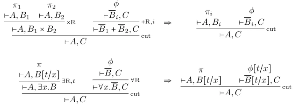
Cut-elimination rules for all1 are given in Figure 6; the requisite permutations are in Figure 7. ∃v.P ∀x.∃y.∀z. P [f (x)/y,z/v] ∃x.∀y.∃z. P P [t/x,g(y)/z] ∃v.P P ⇒ [g(f (t))/v]
We use the example above to illustrate the composition of links. To eliminate the central cut, on∀x.∃y.∀z.P and ∃x.∀y.∃z.P, the explicit substitutions for both formulas must be effectuated. An inductive procedure, as in sequent calculus, could apply them from outside in: first[t/x], then [f(t)/y] (previously [f(x)/y]), then [g(f(t))/z] (previously [g(y)/z]).
For a direct definition, to compose two links (a, b)σ and(b, c)τ, the substitutions into the cut-formula σb and τb must be applied as often as needed, up to the depth of quantifiers
π1 ⊢A, B1 π2 ⊢A, B2 ⊢A, B1× B2 ×R φ ⊢Bi, C ⊢B1+ B2, C +R,i ⊢A, C cut ⇒ πi ⊢A, Bi φ ⊢Bi, C ⊢A, C cut π ⊢A, B[t/x] ⊢A, ∃x.B ∃R,t φ ⊢B, C ⊢∀x.B, C∀R ⊢A, C cut ⇒ π ⊢A, B[t/x] φ[t/x] ⊢B[t/x], C ⊢A, C cut
Figure 6 all1 cut-elimination steps.
⊢A, B ⊢∀x.A, B∀R ⊢B, C ⊢∀x.A, C cut ⊢A[t/x], B ⊢∃x.A, B ∃R,t ⊢B, C ⊢∃x.A, C cut ∼ ∼ ⊢A, B ⊢B, C ⊢A, C cut ⊢∀x.A, C∀R ⊢A[t/x], B ⊢B, C ⊢A[t/x], C cut ⊢∃x.A, C ∃R,t ⊢Ai, B ⊢A1+A2, B +R,i ⊢B, C ⊢A1+A2, C cut ⊢A1, B ⊢A2, B ⊢A1×A2, B ×R ⊢B, C ⊢A1×A2, C cut ∼ ∼ ⊢Ai, B ⊢B, C ⊢Ai, C cut ⊢A1+A2, C +R,i ⊢A1, B ⊢B, C ⊢A1, C cut ⊢A2 , B ⊢B, C ⊢A2, C cut ⊢A1×A2, C ×R ⊢A, B ⊢B, C ⊢A, C cut ⊢C, D ⊢A, D cut ∼ ⊢A, B ⊢B, C ⊢C, D ⊢B, D cut ⊢A, D cut Figure 7 Cut-permutations.
above b, to the terms in the range of the remaining substitutions, σa and τc. To formalize this, we will use the following notions:
The domain-preserving composition of two witness maps σ⋅τ is the map (στ)∣dom(σ). The least fixed point σ of a witness map σ is the least map ρ satisfying ρ= ρσ. The latter is the shortest sequence σ= σσ . . . σ such that no variable is both in the domain and range of σ. This is not necessarily finite; in our composition operations, finiteness is ensured by the correctness conditions on proof nets (see Theorem 15).
IDefinition 14. The composition (A, B)πσ;(B, C)φτ of two proof links is(A, C)ψρ where
ρ= σAτC⋅ σBτB and ψ= ( π ⊢Aσ, Bσ)σBτB ( φ ⊢Bτ, Cτ)σBτB ⊢Aρ, Cρ cut .
The composition λΠΣ; κΦΘ of two linkings is the linking { (X, Y )π σ;(Y , Z) φ τ ∣ (X, Y ) π σ∈ λ Π Σ , (Y , Z) φ τ∈ κ Φ Θ } The composition(λΠ Σ▷ A, B) ; (κ Φ
Θ▷ B, C) of two pre-nets is the pre-net (λ Π Σ; κ
Φ
Θ) ▷ A, C.
These compositions may omit proof annotations and witness annotations.
The composition of two links is strongly related to composition of strategies in game semantics. There, two strategies on⊢A, B and ⊢B, C are composed by interaction on the interface of B and B, and subsequently hiding that interaction.
In the following we will demonstrate that composition gives the desired result: if a net L sequentializes to π and R to φ, then L ; R sequentializes to a normal form of the composition of π and φ with a cut. To this end we will explore how composition and sequentialization interact. We will consider the critical pairs of sequentialization(→) with composition (⇒) given in Figures 8–10, and demonstrate how they are resolved.
⊢A, B1×B2;⊢B1+B2, C (Figure 8)
Since the free existential variables of B and B1are the same, σBτB= σB1τB1 and ρ= ρ
′. It then follows that ψ′ cut-eliminates in one step to ψ.
⊢A, ∃x.B ; ⊢∀x.B, C (Figure 9)
Since x is not free in the range of τ , nor in the range of σ (by Barendregt’s convention), we have that σBτB is(σB− x)τB plus the substitution[σ(x)/x]. Then ρ = ρ′ (as x does not occur in the range of σAτC) and ψ′ reduces to ψ in a single cut-elimination step. ⊢A, B ; ⊢B, ∃x.C (Figure 10)
Observe that since x occurs in C but not B, it is not in the domain of τB, so that τB− x is just τB. Then ρ′= ρ − x, and the diagram is closed by a sequentialization step (from left to right) which extends ψ with an existential introduction rule, to a proof equivalent to ψ′:
ψ
⊢Aρ, Cρ
⊢Aρ′,∃x.Cρ′∃R,ρ(x)
There are three further critical pairs, for a proof net on ⊢A, B composed with one on ⊢B, C1+C2, one on ⊢B, C1×C2, and one on ⊢B, ∀x.C. These converge like the one above. Resolving these critical pairs gives the soundness of the composition operation, per the following theorem. We abbreviate a cut on proofs π⊢A, B and φ ⊢B, C by π ; φ.
ITheorem 15. If proof nets λΣ▷ A, B and κΘ▷ B, C sequentialize to π and φ respectively,
then their composition (λΣ▷ A, B) ; (κΘ▷ B, C) is well-defined (i.e. all fixed points are
finite) and sequentializes to a normal form ψ of π ; φ.
5
Unification nets
In this final section we explore a second notion of all1 proof net: unification nets omit any witness information, which is then reconstructed by coalescence. This yields a natural notion of most general proof net, where every other proof net is obtained by introducing more witness information. Conversely, every witness net has an underlying unification net, that sequentializes to a most general proof.
We consider a proof π⊢A, B more general than π′⊢A, B, written π ≤ π′, if there is a substitution map ρ such that πρ= π′. Unlike for proof nets, this notion is not so natural for
A B1× B2 π,σ π′,σ B1+ B2 C φ,τ → → A B1× B2 π′′,σ B1+ B2 C φ′,τ ⇓ ⇓ A C ψ,ρ A C ψ′,ρ′ ρ = σAτC⋅ σBτB ρ′= σ AτC⋅ σB1τB1 ψ = ( π ⊢Aσ, B1σ) σ B1τB1 ( φ ⊢B1τ, Cτ) σ B1τB1 ⊢Aρ, Cρ cut ψ′= ⎛ ⎜ ⎝ π ⊢Aσ, B1σ π′ ⊢Aσ, B2σ ⊢Aσ, B1σ× B2σ ⎞ ⎟ ⎠σBτB ⎛ ⎜ ⎝ φ ⊢B1τ, Cτ ⊢B1τ+ B2τ, Cτ ⎞ ⎟ ⎠σBτB ⊢Aρ′, Cρ′ cut
Figure 8 The critical pair ⊢A, B1×B2 ; ⊢B1+B2, C.
A ∃x.B π,σ ∀x.B C φ,τ → x ∉ τ → A ∃x.B π′,σ−x ∀x.B C φ′,τ ⇓ ⇓ A C ψ,ρ A C ψ′,ρ′ ρ = σAτC⋅ σBτB ρ′= σ AτC⋅ (σB− x)τB ψ = ( π ⊢Aσ, Bσ) σBτB ( φ ⊢Bτ, Cτ) σBτB ⊢Aρ, Cρ cut ψ′= ⎛ ⎜ ⎝ π ⊢Aσ, Bσ ⊢Aσ, ∃x.Bσ − x ⎞ ⎟ ⎠(σB− x)τB ⎛ ⎜ ⎝ φ ⊢Bτ, Cτ ⊢∀x.Bτ, Cτ ⎞ ⎟ ⎠(σB− x)τB ⊢Aρ′, Cρ′ cut
Figure 9 The critical pair ⊢A, ∃x.B ; ⊢∀x.B, C.
A B π,σ B ∃x.C φ,τ → A B π,σ B ∃x.C φ′ ,τ −x ⇓ ⇓ A ∃x.C ψ,ρ A ∃x.C ψ′,ρ′ ρ = σAτC⋅σBτB ρ′ = σA(τC−x) ⋅ σBτB ψ = ( π ⊢Aσ, Bσ )σBτB ( φ ⊢Bτ, Cτ )σBτB ⊢Aρ, Cρ cut ψ′ = ( π ⊢Aσ, Bσ )σBτB ⎛ ⎜ ⎜ ⎝ φ ⊢Bτ, Cτ ⊢Bτ, ∃x.C(τ − x) ⎞ ⎟ ⎟ ⎠ σBτB ⊢Aρ′, ∃x.Cρ′ cut
sequent proofs: in the permutation of existential and product rules below, from left to right
u must be generated as the least term more general than s and t; from right to left, s and t
cannot be reconstructed from u, and must be retrieved from their respective subproofs. ⊢A, C ⊢A, ∃x.C∃R,s ⊢B, ∃x.C⊢B, C ∃R,t ⊢A × B, ∃x.C ×R ∼ ⊢A, C ⊢B, C ⊢A × B, C ×R ⊢A × B, ∃x.C∃R,u
To reconstruct witnesses by unification, we define the following operations.
σ≤ τ : A witness map σ is more general than τ if there is a map ρ such that σρ = τ. σ a τ : Two witness maps σ and τ are coherent if there is a map ρ such that σρ= τρ. σ∨ τ : The join of coherent witness maps is the least map ρ such that σ ≤ ρ and τ ≤ ρ.
A link(a, b) on two atomic formulas is an axiom link if there exists a witness map σ such that aσ= bσ. To an axiom link (a, b) over ⊢A, B we assign an initial witness map, which is the least witness map σ over the domain evA(a) ∪ evB(b) such that aσ = bσ. In other words, σ is the most general unifier of a and b, over the given domain, written mgu(a, b). For an axiom linking λ over⊢A, B the initial witness pre-net λ⋆▷ A, B is given by
λ⋆= { (a, b)σ ∣ (a, b) ∈ λ , σ = mgu(a, b) } .
An initial witness pre-net has exact coverage, while coalescence will give local eigenvariables. Note that eigenvariables are constants for the purpose of unification (they are not substituted into). For Barendregt’s convention, that free variables have distinct names from bound ones, we should assume that variables in the range of a witness map are fresh; for example, the most general unifier of existential variables x and y should be[z/x, z/y] for a fresh variable z, and not[y/x] or [x/y].
IDefinition 16. Unifying sequentialization ( ) is the rewrite relation on labelled
pre-nets generated by the rules(+U, i), (∃U), (∀U), which are respectively as (+S, i), (∃S), and
(∀S), and the rule (C, D1)πσ (C, D2)φτ} (C, D 1×D2) ψ σ∨τ = σρ = τ ρ (σaτ ) ψ= ( π ⊢Aσ, Bσ)ρ (⊢Aτ, Cτ)φ ρ ⊢A(σ∨τ), Bσρ × Cτρ (×U)
Unifying coalescence is the relation ( ) on witness pre-nets, ignoring proof labels. A witness pre-net λΣ▷A, B unifying-coalesces if it reduces to {(A, B)∅}▷A, B and strongly
unifying-coalesces if any coalescence path terminates at{(A, B)∅} ▷ A, B.
IDefinition 17. An all1 unification proof net or unification net is a pre-net λ▷A, B
with axiom linking λ such that the initial witness pre-net λ⋆▷ A, B unifying-coalesces. It
sequentializes to π if λ⋆
⋆▷ A, B reduces in ( ) to {(A, B) π
∅} ▷ A, B. In the above definition, note that λ⋆
⋆ = (λ⋆)
⋆ is the initial proof labelling of λ
⋆, which assigns an axiom rule to each axiom link. For a minimal example, see the Introduction. Observe also that unifying coalescence includes strict coalescence,(→) ⊆ ( ). The following two lemmata relate sequentialization for witness nets and unification nets.
I Lemma 18. In ( ), if λΣ▷ A, B sequentializes to π then λ⋆▷ A, B sequentializes to
π′≤ π.
ILemma 19. If λ⋆▷A, B unifying-sequentializes to π then there exists a witness assignment Σ and substitution ρ such that λΣ▷ A, B strict-sequentializes to π and λΣ= λ⋆ρ.
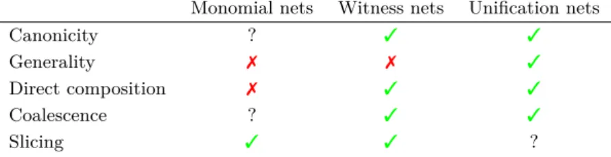
Monomial nets Witness nets Unification nets Canonicity ? 3 3 Generality 7 7 3 Direct composition 7 3 3 Coalescence ? 3 3 Slicing 3 3 ?
Figure 11 Comparison of different notions of proof nets for quantifiers and additive connectives.
We can then show that sequentialization and de-sequentialization for unification nets are inverses up to generality, and that composition is sound.
ITheorem 20. If [π ⊢A, B] is λΣ▷ A, B then λ ▷ A, B unifying-sequentializes to π′≤ π.
ITheorem 21. If λ▷ A, B sequentializes to π, then [π] = λΣ▷ A, B for some Σ.
ITheorem 22. If λ▷ A, B sequentializes to π and κ ▷ B, C to φ then their composition
λ ; κ▷ A, C sequentializes to a proof ψ′≤ ψ where ψ is a normal form of π ; φ.
6
Conclusion and related work
We have presented two notions of first-order additive proof net, witness nets and unification
nets, to capture canonically two natural notions of proof identity for first-order additive
linear logic. Figure 11 summarizes our results, along with some observations we make below. Proof nets with additives and quantifiers existed before as monomial nets [8]. These are not generally canonical: they admit the permutation (and duplication) of proof rules past implicit contractions (that is, the shared context of the additive conjunction rule). However, it might be possible to restrict additive monomial nets to some notion of canonical form. Likewise, coalescence (or contractibility) has not been studied for first-order monomial nets, though it has been extended to a related form of MALL proof nets [24].
Our slicing condition is loosely related to a number of approaches to first-order classical logic. A formula∃x.A is interpreted as the sum (or classically, the disjunction) over a fixed number of instantiations A[t1/x] + . . . + A[tn/x]. This can be traced to Herbrand’s Theorem [14]: ∃x.A is equivalent to the infinite sum over A[t/x] for all terms t in the language, but for any given proof a finite set of terms suffices. Expansion tree proofs [25, 10] are a graphical proof formalism based on this idea. In our slicing condition, the interpretation of∃x.A is an infinite sum of which only a finite part A[t1/x] + . . . + A[tn/x] is relevant, over the witnesses
t1, . . . , tn actually assigned to x in the proof net. An interesting alternative approach to additive proof nets, which we may explore in future work, is to take the expansion of∃x.A to A[t1/x] + . . . + A[tn/x] as primary, and record it explicitly in the syntax, as expansion tree proofs do for classical logic. It is expected, however, that this would sacrifice generality and
direct composition.
Hetzl [15] explores explicit substitution for first-order classical sequent calculus.
Lambek observed that the two canonical proofs of ⊢A+A, A can be distinguished by casting each as a specialization (by substituting into propositional variables) of the more general proofs of⊢ a+b, a and ⊢ a+b, b (corresponding to the two injections of a sum). He proposed to use this idea of generality as the basis for a notion of proof identity: two proofs are equivalent if their most general forms are isomorphic [23]. How this extends to first order is not obvious. The natural first-order analogue of⊢A+A, A would be ⊢∃x.A, A where the quantifier is vacuous, as∃x.A represents the infinite sum over A (for all terms t). Where
Lambek’s generality distinguishes the two proofs of⊢A+A, A, ours identifies the proofs of ⊢∃x.A, A: the sequent has one unification net, but infinitely many witness nets (one for each term t). If existential quantification is indeed analogous to a sum, Lambek’s notion of generality is more faithfully captured by witness nets than unification nets.
For future work, there are a few natural questions. First is that of a geometric criterion for unification nets. For this, it seems essential to reconstruct dependencies between products and existential quantifiers globally, as the expansion condition provides for witness nets. These interact in highly intricate ways, which the unifying coalescence algorithm resolves incrementally and locally. To do so globally, as would be necessary for a geometric criterion, is a major combinatorial challenge.
A second is whether coalescence (or contractibility [4]) applies to MLL1 unification nets [18]. We believe it would, straightforwardly (without requiring a dependency or leap edges).
A final question is whether the current approach can be extended to obtain proof nets for MALL1. We see two ways forward that could succeed: (i) combine witness nets with MALL slice nets [21] using a slicing criterion; (ii) combine witness nets or unification nets with MALL conflict nets [20] using a coalescence criterion. For both, there are still significant combinatorial challenges, for example because coalescence for MALL is not a straightforward extension of that for ALL. Other approaches are much less certain: MALL conflict nets do not yet have a slicing criterion (though this looks feasible), and MALL slice nets do not support coalescence (which seems fundamentally problematic).
References
1 Samson Abramsky. Sequentiality vs. Concurrency in Games and Logic. Mathematical Structures in Computer Science, 13(4):531–565, 2003.
2 Luís Caires and Frank Pfenning. Session types as intuitionistic linear propositions. In CONCUR, volume 6269 of LNCS, pages 222–236, 2010.
3 Robin Cockett and Luigi Santocanale. On the Word Problem for ΣΠ-Categories, and the Properties of Two-Way Communication. In Computer Science Logic (CSL), 18th Annual Conference of the EACSL, pages 194–208, 2009.
4 Vincent Danos. La Logique Linéaire appliquée à l’étude de divers processus de normalisation (principalement du Lambda-calcul). PhD thesis, Université Paris 7, 1990.
5 Vincent Danos and Laurent Regnier. The structure of multiplicatives. Archive for Mathematical Logic, 28:181–203, 1989.
6 Didier Galmiche and Jean-Yves Marion. Semantic Proof Search Methods for ALL – a first approach –. Short paper in Theorem Proving with Analytic Tableaux, 4th International Workshop (TABLEAUX’95). Available from the first author’s webpage, 1995.
7 Jean-Yves Girard. Linear Logic. Theoretical Computer Science, 50(1):1–102, 1987.
8 Jean-Yves Girard. Proof-nets: the parallel syntax for proof-theory. Logic and Algebra, pages 97–124, 1996.
9 Stefano Guerrini and Andrea Masini. Parsing MELL proof nets. Theoretical Computer Science, 254(1-2):317–335, 2001.
10 Willem Heijltjes. Classical proof forestry. Ann. Pure Appl. Logic, 161(11):1346–1366, 2010.
11 Willem Heijltjes. Proof nets for additive linear logic with units. In 26th Annual IEEE Symposium on Logic in Computer Science (LICS), pages 207–216, 2011.
12 Willem Heijltjes and Dominic J. D. Hughes. Complexity bounds for sum–product logic via additive proof nets and Petri nets. In 30th Annual ACM/IEEE Symposium on Logic in Computer Science (LICS), pages 80–91, 2015.
13 Willem Heijltjes, Dominic J. D. Hughes, and Lutz Straßburger. Proof nets for first-order addit-ive linear logic. Technical Report RR-9201, INRIA, 2018. URL: hal.inria.fr/hal-01867625/.
14 Jacques Herbrand. Investigations in proof theory: The properties of true propositions. In Jean van Heijenoort, editor, From Frege to Gödel: A source book in mathematical logic, 1879–1931, pages 525–581. Harvard University Press, 1967.
15 Stefan Hetzl. A sequent calculus with implicit term representation. In Computer Science Logic (CSL), volume 6247 of LNCS, pages 351–365, 2010.
16 Kohei Honda, Vasco Vasconcelos, and Makoto Kubo. Language primitives and type disciplines for structured communication-based programming. In European Symposium on Programming, pages 122–138, 1998.
17 Dominic J. D. Hughes. Proofs Without Syntax. Annals of Mathematics, 164(3):1065–1076, 2006.
18 Dominic J. D. Hughes. Unification nets: canonical proof net quantifiers. In 33rd Annual ACM/IEEE Symposium on Logic in Computer Science (LICS), 2018.
19 Dominic J. D. Hughes. First-order proofs without syntax. Available at arXiv.org, 2019.
20 Dominic J. D. Hughes and Willem Heijltjes. Conflict nets: efficient locally canonical MALL proof nets. In 31st Annual ACM/IEEE Symposium on Logic in Computer Science (LICS), 2016.
21 Dominic J. D. Hughes and Rob van Glabbeek. Proof nets for unit-free multiplicative-additive linear logic. Transactions on Computational Logic, 6(4):784–842, 2005.
22 Andre Joyal. Free Lattices, Communication and Money Games. Proc. 10th Int. Cong. of Logic, Methodology and Philosophy of Science, 1995.
23 Joachim Lambek. Deductive Systems and Categories I, II, III. Theory of Computing Systems (I), Lecture Notes in Mathematics (II, III), 1968–1972.
24 Roberto Maieli. Retractile Proof Nets of the Purely Multiplicative and Additive Fragment of Linear Logic. In 14th Int. Conf. Logic for Programming Artificial Intelligence and Reasoning (LPAR), pages 363–377, 2007.
25 Dale Miller. A Compact Representation of Proofs. Studia Logica, 46(4):347–370, 1987.
26 Samuel Mimram. The Structure of First-Order Causality. Mathematical Structures in Computer Science, 21(1):65–110, 2011.
27 Lutz Straßburger. A Characterisation of Medial as Rewriting Rule. In Franz Baader, editor, Term Rewriting and Applications, RTA’07, volume 4533 of LNCS, pages 344–358, 2007.
28 Philip Wadler. Propositions as Sessions. Journal of Functional Programming, 24(2-3):384–418, 2014.
A
Proofs
In this appendix we restate and prove all theorems, and add two supporting lemmata.
ITheorem 6. For any all1 proof π, the witness net [π] sequentializes to π.
Proof. It follows by induction on π that if λΣ= [π ⊢A, B]A
′,B′
σ where A
′σ= A and B′σ= B, then λ⋆
Σ▷ A, B reduces in (→) to {(A
′, B′)πσ} ▷ A, B. The statement is the case σ = ∅.
J ITheorem 7. If λΣ▷ A, B sequentializes to π, then [π] is λΣ▷ A, B.
Proof. By induction on the sequentialization path λ⋆
Σ▷ A, B →
∗ {(A, B)π
∅} ▷ A, B it fol-lows that in every pre-net κΦΘ▷ A, B on this path, λΣ is equal to the union over the de-sequentialization of all proof labels φ in Φ:
λΣ= ⋃ { [φ]C,Dσ ∣ (C, D) φ σ∈ κ
Φ Θ} .
The statement is then the case κΦΘ= {(A, B)π∅}. J
Proof. From left to right is by inspection of the critical pairs of sequentialization (→). From right to left is by inspection of the rule permutations in Figure 2. J
ILemma 23. Strict coalescence preserves and reflects correctness.
Proof. For a strict coalescence step L→ R, we will show that the witness pre-net L is correct if and only if R is. Let L= λΣ▷ A, B and R = κΘ▷ A, B. In each case, exact coverage and local eigenvariables are immediately preserved and reflected. For slice-correctness, we will demonstrate that the left-hand side and right-hand side of each rule belong to the same slice of⊢A, B, or in the case of ∃S, naturally corresponding slices. For dependency-correctness, we will briefly show how acyclicity of the columns of the involved links is preserved.
(C, Di)σ→ (C, D1+D2)σ
A slice SB of B and ∅ containing one of (D1, τ), (D2, τ), and (D1+ D2, τ) must also contain the other two. A slice S of ⊢A, B then contains all three of (C, D1)σ, (C, D2)σ, and (C, D1+D2)σ, or none. It follows that S∩ λΣ is a singleton if and only if S∩ κΘ is. Since other slices are unaffected, L is slice-correct if and only if R is.
For dependency-correctness, the column of(C, Di)σ is that of(C, D1+D2)σplus the pair (Di, σ∣evB(Di)) itself, which is minimal in the order 4.
(C, D1)σ,(C, D2)σ→ (C, D1×D2)σ
A slice S of⊢A, B contains (C, D1×D2)σ if and only if it contains either of (C, D1)σ or (C, D2)σ, and cannot contain both. Then S∩ λΣis a singleton if and only if S∩ κΘ is. Dependency-correctness is immediate, as above.
(C, D)σ→ (C, ∃x.D)σ−x
A slice S of ⊢A, B contains (C, ∃x.D)τ if and only if it contains all links(C, D)τ [t/x] for any term t. Letting τ[t/x] = σ, then S ∩ λΣ is the singleton{(C, D)σ} if and only if
S∩ κΘ is{(C, ∃x.D)σ−x}.
For dependency-correctness, the column of (C, D)σ is that of (C, ∃x.D)σ−x plus a pair (D, τ), which is minimal in (4).
(C, D)σ→ (C, ∀x.D)σ
A slice S of⊢A, B contains (C, D)σ if and only if it contains also(C, ∀x.D)σ, and hence
S∩ λΣis a singleton if and only if S∩ κΘ is.
For dependency-correctness, the column of (C, D)σ is that of (C, ∀x.D)σ plus a pair (D, τ). The side-condition of the coalescence step is that x ∉ σ; then x does not occur
free in any (X, ρ), and (D, τ) is minimal in (4). J
ILemma 24. To a correct witness pre-net λΣ▷ A, B a coalescence step applies, unless it is
fully coalesced already, λΣ= {(A, B)∅}.
Proof. Let the depth of a link(C, D)σbe a pair of integers (n, m), where n is the distance from C to the root of A, and m that from D to B. We order link depth in the product order: (i, j) ≤ (n, m) if and only if i ≤ n and j ≤ m. We will demonstrate that a link at maximal depth may always be coalesced, unless it is the unique link(A, B)∅ at(0, 0).
To see that a maximally deep link coalesces, first note that a link (C, Di)σ where Di occurs in D0+D1 may always coalesce, as may a link(C, D)σ where D occurs in∃x.D. This leaves the following cases:
(A, Di)σ with Di occurring in D= D1× D2.
Without loss of generality, let i= 1. A slice S1 of ⊢A, B containing (A, D1)σ has a counterpart S2 containing (A, D2)σ. The depth of (A, D2)σ is the same as that of (A, D1)σ. By correctness S2∩ λΣ is a singleton; by the assumption of maximality it
may not contain a deeper link than (A, D2)σ; and it may not contain a shallower one since that would be shared with S1∩ λΣ. Then λΣ▷ A, B contains both (A, D1)σ and (A, D2)σ, and these contract to(A, D)σ.
(A, D)σ with D in∀x.D.
The step (A, D)σ→ (A, ∀x.D)σ applies if x∉ σ. By way of contradiction, assume x ∈ σ. The column of (A, D)σ contains(D, σD) and (∀x.D, τ) where τ = σ∣evB(∀x.D). By the exact coverage condition, σ= σA∪ σD, and since the free existential variables in D and ∀x.D are the same, evB(D) = evB(∀x.D), so that τ = σD. (Note that since σA= ∅, we get σ= σD= τ, but this is not essential to the argument.) Since x ∈ σ we have x ∈ τ, and in the column of(A, D)σ we have(∀x.D, τ) 4 (D, τ) since D occurs as ∀x.D. But we already have(D, τ) 4 (∀x.D, τ) because D ≤ ∀x.D, contradicting antisymmetry of (4). Then x∉ σ, and the step (A, D)σ→ (A, ∀x.D)σ applies.
(Ci, Dj)σ in C= C1× C2and D= D1× D2.
Without loss of generality, let i= j = 1. By minimal depth and using similar reasoning to the first case above, the pre-net must contain one of the following three configurations.
1. (C1, D1)σ, (C1, D2)σ, (C2, D1)σ, (C2, D2)σ 2. (C1, D1)σ, (C1, D2)σ, (C2, D)σ 3. (C1, D1)σ, (C2, D1)σ, (C, D2)σ 1∶ C1×C2 D1×D2 2∶ C1×C2 D1×D2 3∶ C1×C2 D1×D2 In the second case, the step(C1, D1)σ,(C1, D2)σ→ (C1, D)σ applies; in the third case, (C1, D1)σ,(C2, D1)σ→ (C, D1)σ; and in the first case, both.
(Ci, D)σ in C= C1× C2and ∀x.D.
Without loss of generality let i= 1. If x ∉ σ the rewrite step (C1, D)σ→ (C1,∀x.D)σ applies. Otherwise, let x∈ σ. The slice S1of⊢A, B containing (C1, D)σhas a counterpart
S2 containing(C2, D)σ, which must include exactly one link of λΣ. By the assumption of minimal depth, it cannot have greater depth than(C2, D)σ. It cannot be(C, D)σ or any shallower link, since that would be shared with the slice S1 which already contains (C1, D)σ. It cannot be(C2,∀x.D)σ or any shallower link(C2, X)τ (i.e. with ∀x.D ≤ X) because x∈ σ. This would mean either x ∈ τ which contradicts the eigenvariables not free convention, or x∈ fv(σ(y)) where ∀x.D < ∃y.Y ≤ X which creates a cyclic column, as in the second case above. It follows that S2∩ λΣ= {(C2, D)σ}, so that the rewrite step (C1, D)σ,(C2, D)σ→ (C, D)σ applies.
(C, D)σ in ∀x.C and ∀y.D.
A rewrite step (C, D)σ → (∀x.C, D)σ or(C, D)σ → (C, ∀y.D)σ applies unless x, y ∈ σ. But that would generate a cycle in the column of(C, D)σ, in one of three ways. If x∈ σC or y∈ σDthen, since σC= σ∀x.C and σD= σ∀y.D, respectively:
(C, σC) 4 (∀x.C, σC) 4 (C, σC) (D, σD) 4 (∀y.D, σD) 4 (D, σD) . Otherwise, if x∈ σD and y∈ σC then
(C, σC) 4 (∀x.C, σC) 4 (D, σD) 4 (∀x.D, σD) 4 (C, σC) . J
I Theorem 12. A witness pre-net that strict-coalesces is correct, and a correct witness
pre-net strongly strict-coalesces.
Proof. For the first statement, we proceed by induction on the coalescence path from
λΣ▷ A, B to {(A, B)∅} ▷ A, B, with the end result as the base case. It is slice-correct: every slice of⊢A, B contains (A, B)∅, so every slice of {(A, B)∅} ▷ A, B is the singleton {(A, B)∅}. It is also dependency-correct: the column of (A, B)∅ is the set{(A, ∅), (B, ∅)}, where A and B are unrelated in (4). For the inductive step, by Lemma 23 coalescence
reflects correctness, so that any pre-net along the coalescence path is correct, in particular
λΣ▷ A, B.
For the second statement, let λΣ▷ A, B be correct. By Lemma 24 either the net has coalesced, or a coalescence step applies. By Lemma 23 the result of any coalescence step is again correct. Since links strictly move towards the roots of both formula trees, it follows that this process terminates, and the pre-net λΣ▷ A, B strongly strict-coalesces. J
ITheorem 15. If proof nets λΣ▷ A, B and κΘ▷ B, C sequentialize to π and φ respectively,
then their composition (λΣ▷ A, B) ; (κΘ▷ B, C) is well-defined (i.e. all fixed points are
finite) and sequentializes to a normal form ψ of π ; φ.
Proof. By Theorem 12 the proof nets L= λΣ▷ A, B and R = κΘ▷ B, C strongly coalesce. We may then interleave their coalescence sequences as follows: if a synchronized step in L and R on the interface B and B is available, apply it; otherwise perform steps in L on A and in R on C until it is. This gives the following combined sequence.
L = L1 →? L2 →? . . . →? Ln
R = R1 →? R2 →? . . . →? Rn
⇓ ⇓ ⇓ ⇓
L ; R = L1; R1 → L2; R2 → . . . → Ln; Rn
(Here,(→?) is the relation (→) ∪ (=), but we assume that at least L
i→ Li+1or Ri→ Ri+1.) The path along the top and right of this diagram sequentializes L to π′and R to φ′(equivalent to π and φ respectively), and then composes to Ln; Rn= {(A, C)π∅′;φ′} ▷ A, C.
Each square of the diagram converges as one of the critical pairs of sequentialization and composition discussed above. Then each path along the diagram from top left (L and
R) to bottom right(Ln; Rn) gives a sequentialization, with cuts, of Ln; Rn. Let the path taking the vertical step from Li and Ri to Li; Ri sequentialize to ψi, so that ψn= ψ′. By the way each square converges, we have that ψi is reached from ψi+1 by a cut-elimination or permutation step.
Finally, in L and R every link is an axiom link. Any link in L ; R is composed from two links (a, b)σ in L and (b, c)τ in R, which yields (a, c)ρ where ρ = σaτc⋅ σbτb. This sequentializes to the axiom⊢aρ, cρ, which is in normal form. Then L ; R is a proof net (it has an axiom linking and it coalesces), and it sequentializes to a normal form of ψ. J
I Lemma 18. In ( ), if λΣ▷ A, B sequentializes to π then λ⋆▷ A, B sequentializes to
π′≤ π.
Proof. The sequentialization path λ⋆
Σ▷ A, B = L1 L2 . . . Ln= (A, B)π∅▷ A, B has a corresponding path λ⋆
⋆▷ A, B = R1 R2 . . . Rn= (A, B) π′
∅▷ A, B where the same links (but with potentially different witness maps) are coalesced. It follows by induction on this path (where the base case is L1and R1) that for every corresponding pair of links (C, D)φ
σ in Li and(C, D) ψ
τ in Ri we have τ ≤ σ and ψ ≤ φ. J
ILemma 19. If λ⋆▷A, B unifying-sequentializes to π then there exists a witness assignment Σ and substitution ρ such that λΣ▷ A, B strict-sequentializes to π and λΣ= λ⋆ρ.
Proof. By induction on the sequentialization path λ⋆▷ A, B
∗(A, B)π
∅▷ A, B. For the end result, the statement holds with ρ= ∅. For the inductive step, consider a step L R. We show the case (×U); the other cases are immediate.