Cloud type comparisons of AIRS, CloudSat, and CALIPSO cloud height and amount

(1)

HAL Id: hal-00303111

https://hal.archives-ouvertes.fr/hal-00303111

Submitted on 27 Sep 2007

HAL is a multi-disciplinary open access

archive for the deposit and dissemination of sci-entific research documents, whether they are pub-lished or not. The documents may come from teaching and research institutions in France or abroad, or from public or private research centers.

L’archive ouverte pluridisciplinaire HAL, est destinée au dépôt et à la diffusion de documents scientifiques de niveau recherche, publiés ou non, émanant des établissements d’enseignement et de recherche français ou étrangers, des laboratoires publics ou privés.

Cloud type comparisons of AIRS, CloudSat, and

CALIPSO cloud height and amount

B. H. Kahn, M. T. Chahine, G. L. Stephens, G. G. Mace, R. T. Marchand, Z.

Wang, C. D. Barnet, A. Eldering, R. E. Holz, R. E. Kuehn, et al.

To cite this version:

B. H. Kahn, M. T. Chahine, G. L. Stephens, G. G. Mace, R. T. Marchand, et al.. Cloud type comparisons of AIRS, CloudSat, and CALIPSO cloud height and amount. Atmospheric Chemistry and Physics Discussions, European Geosciences Union, 2007, 7 (5), pp.13915-13958. �hal-00303111�

(2)

ACPD

7, 13915–13958, 2007

AIRS, CloudSat, and CALIPSO clouds B. H. Kahn et al. Title Page Abstract Introduction Conclusions References Tables Figures ◭ ◮ ◭ ◮ Back Close

Full Screen / Esc

Printer-friendly Version

Interactive Discussion

EGU

Atmos. Chem. Phys. Discuss., 7, 13915–13958, 2007 www.atmos-chem-phys-discuss.net/7/13915/2007/ © Author(s) 2007. This work is licensed

under a Creative Commons License.

Atmospheric Chemistry and Physics Discussions

Cloud type comparisons of AIRS,

CloudSat, and CALIPSO cloud height and

amount

B. H. Kahn1, M. T. Chahine1, G. L. Stephens2, G. G. Mace3, R. T. Marchand4, Z. Wang5, C. D. Barnet6, A. Eldering1, R. E. Holz7, R. E. Kuehn8, and D. G. Vane1

1

Jet Propulsion Laboratory, California Institute of Technology, Pasadena, CA, USA

2

Department of Atmospheric Science, Colorado State University, Fort Collins, CO, USA

3

Department of Meteorology, University of Utah, Salt Lake City, UT, USA

4

Joint Institute for the Study of the Atmosphere and Ocean, University of Washington, Seattle, WA, USA

5

Department of Atmospheric Science, University of Wyoming, Laramie, WY, USA

6

NOAA–NESDIS, Silver Springs, MD, USA

7

CIMSS–University of Wisconsin–Madison, Madison, WI, USA

8

NASA Langley Research Center, Hampton, VA, USA

Received: 14 September 2007 – Accepted: 17 September 2007 – Published: 27 September 2007

(3)

ACPD

7, 13915–13958, 2007

Full Screen / Esc

EGU Abstract

The precision of the two-layer cloud height fields derived from the Atmospheric Infrared Sounder (AIRS) is explored and quantified for a five-day set of observations. Coincident profiles of vertical cloud structure by CloudSat, a 94 GHz profiling radar, and the Cloud-Aerosol Lidar and Infrared Pathfinder Satellite Observation (CALIPSO), are compared 5

to AIRS for a wide range of cloud types. Bias and variability in cloud height differences are shown to have dependence on cloud type, height, and amount, as well as whether CloudSat or CALIPSO is used as the comparison standard. The CloudSat–AIRS bi-ases and variability range from −4.3 to 0.5±1.2–3.6 km for all cloud types. Likewise, the CALIPSO–AIRS biases range from 0.6–3.0±1.2–3.6 km (−5.8 to −0.2±0.5–2.7 km) 10

for clouds ≥7 km (<7 km). The upper layer of AIRS has the greatest sensitivity to Al-tocumulus, Altostratus, Cirrus, Cumulonimbus, and Nimbostratus, whereas the lower layer has the greatest sensitivity to Cumulus and Stratocumulus. Although the bias and variability generally decrease with increasing cloud amount, the ability of AIRS to con-strain cloud occurrence, height, and amount is demonstrated across all cloud types for 15

many geophysical conditions. In particular, skill is demonstrated for thin Cirrus, as well as some Cumulus and Stratocumulus, cloud types infrared sounders typically struggle to quantify. Furthermore, some improvements in the AIRS Version 5 operational re-trieval algorithm are demonstrated. However, limitations in AIRS cloud rere-trievals are also revealed, including the existence of spurious Cirrus near the tropopause and low 20

cloud layers within Cumulonimbus and Nimbostratus clouds. Likely causes of spurious clouds are identified and the potential for further improvement is discussed.

1 Introduction

Improving the realism of cloud fields within general circulation models (GCMs) is nec-essary to increase certainty in prognoses of future climate (Houghton et al., 2001). 25

(4)

ACPD

7, 13915–13958, 2007

Full Screen / Esc

EGU

model to model and are largely attributed to differences in the representation of cloud feedback processes (Stephens, 2005). Use of relatively long-term satellite data records such as the Earth Radiation Budget Experiment (ERBE) (Ramanathan et al., 1989) and the International Satellite Cloud Climatology Project (ISCCP) (Rossow and Schiffer, 1999) have clarified cloud radiative impacts, inspired approaches to climate GCM eval-5

uation, and contributed to further theoretical understanding of cloud feedbacks (e.g., Hartmann et al., 2001). Wielicki et al. (1995) note the historical satellite record is un-able to measure all cloud properties relevant to Earth’s cloudy radiation budget, which include liquid and ice water path (LWP/IWP), visible optical depth (τ), effective particle size (De), particle phase and shape, fractional coverage, height, and IR emittance.

Il-10

lustrating the need for improved cloud observations, Webb et al. (2001) showed that some climate GCMs generate erroneous vertical cloud distributions that compensate in a manner producing favorable mean radiative budget comparisons with observations. Thus, reliable observations of cloud vertical structure will help to reduce the ambiguity in climate GCM–satellite comparisons.

15

Several active and passive satellite sensors with unprecedented observing capabil-ities are flying in a formation called the “A-train” (Stephens et al., 2002). The constel-lation is anchored by NASA’s Earth Observing System (EOS) Aqua and Aura satel-lites, the Cloud-Aerosol Lidar and Infrared Pathfinder Satellite Observation (CALIPSO) (Winker et al., 2003), CloudSat (Stephens et al., 2002), along with the Polarization 20

and Anisotropy of Reflectances for Atmospheric Sciences coupled with Observations from a Lidar (PARASOL), and in the near future Glory (solar irradiance and aerosols), and the Orbiting Carbon Observatory (OCO) (atmospheric CO₂). Several instruments on Aqua and Aura are designed to measure temperature, humidity, clouds, aerosols, trace gases, and surface properties (Parkinson et al., 2003; Schoeberl et al., 2006). 25

The present focus is on comparisons of cloud retrievals from the Atmospheric Infrared Sounder (AIRS) located on Aqua (Aumann et al., 2003) to CloudSat, a 94 GHz cloud profiling radar, and CALIOP (Cloud-Aerosol Lidar with Orthogonal Polarization), a cloud and aerosol profiling lidar on CALIPSO. Aqua leads CloudSat and CALIPSO by ∼55

(5)

ACPD

7, 13915–13958, 2007

Full Screen / Esc

EGU

and ∼70 s, respectively, providing nearly simultaneous and collocated cloud observa-tions.

From the perspective of a satellite-based cloud observation, inter-satellite compar-isons have several advantages over surface-satellite comparcompar-isons: they (1) eliminate the ambiguity introduced from the integration of a time series of surface-based mea-5

surements to replicate a spatial scale comparable to the satellite field of view (FOV) that is further complicated by cloud temporal evolution (e.g., Kahn et al., 2005), (2) reduce the effects of certain types of sampling biases, including those introduced by the attenuation of surface-based lidar and cloud radar in thick and precipitating clouds (Comstock et al., 2002; McGill et al., 2004), (3) provide a larger and statistically robust 10

set of observations for comparison, and (4) facilitate near-global sampling for most types of clouds.

Many schemes have been developed to classify clouds into fixed types. For instance, the ISCCP data set provides a 3×3 classification scheme based on cloud top pressure and τVIS (Rossow and Schiffer, 1999), while Wang and Sassen (2001) developed a

15

scheme using multiple ground-based sensors. These (and numerous other) classifica-tion schemes are loosely based on the naming system originating from Luke Howard (Gedzelman, 1989). Although cloud classification schemes are limited by measure-ment sensitivity and subject to misinterpretation, they help to organize clouds into cate-gories with unique characteristics of composition, radiative forcing, and heating/cooling 20

effects (Hartmann et al., 1992; Klein and Hartmann 1993; Chen et al., 2000; Inoue and Ackerman, 2002; Xu et al., 2005; L’Ecuyer et al., 2006).

No single passive or active measurement from space is able to infer all relevant cloud physical properties (e.g., Wielicki et al., 1995) spanning all geophysical conditions; hence, a multi-instrument constellation is needed to observe Earth’s clouds (Miller et 25

al., 2000; Stephens et al., 2002). Now that this type of satellite constellation is oper-ational, the strengths and weaknesses of various instruments can be evaluated in the presence of different cloud types and ultimately observations of multiple instruments can be combined to yield retrievals superior to retrievals from any single instrument.

(6)

ACPD

7, 13915–13958, 2007

Full Screen / Esc

EGU

This is motivated in part because of discrepancies in existing climatologies of cloud height, frequency and amount derived from combinations of passive (visible, IR, and microwave) wavelengths (e.g., Rossow et al., 1993; Jin et al., 1996; Thomas et al., 2004). Discrepancies exist not only from different measurement characteristics and sampling strategies, but perhaps as significantly, from retrieval algorithm differences 5

and a priori assumptions (Rossow et al., 1985; Wielicki and Parker, 1992; Kahn et al., 2007b). CloudSat and CALIOP generally provide more direct and easily interpreted observations of cloud detection and vertical cloud structure than passive methods. A combination of radiative transfer modeling and a priori assumptions of surface and atmospheric quantities are necessary to infer cloud properties from passive measure-10

ments (e.g. Rossow and Schiffer, 1999).

The scientific literature is replete with cross-comparisons of in situ, surface-based, and satellite-derived cloud properties. However, there are few that consider the im-pacts of cloud type on the distribution of statistical properties. The precision of passive satellite-derived cloud quantities is not only impacted by cloud type, but temperature 15

(Susskind et al., 2006) and water vapor variability (Fetzer et al., 2006), trace gases (Kulawik et al., 2006), aerosols (Remer et al., 2005), and surface quantities have vary-ing degrees of precision within different cloud types. In this article, the accuracy of AIRS cloud height and amount for different cloud type configurations is quantified us-ing CloudSat and CALIPSO. In Sect. 2 the observations and data products of the three 20

observing platforms are introduced. Section 3 describes the comparison methodology and presents illustrative cloud climatologies of AIRS, CloudSat, and CALIOP. Simi-larities and differences are placed in the context of measurement sensitivity. Sect. 4 presents coincident CloudSat–AIRS cloud top differences spanning the breadth of cloud types. CALIPSO–AIRS cloud top differences are shown and compared to those 25

between CloudSat–AIRS. Furthermore, strengths and weaknesses of AIRS cloud re-trievals are revealed and probable causes of discrepancies are discussed. In Sect. 5 the results are discussed and summarized.

(7)

ACPD

7, 13915–13958, 2007

Full Screen / Esc

EGU

2 Data

The sensitivity of radar, lidar and passive IR sounders to clouds differs greatly. Active sensors provide relatively direct observations of cloud vertical structure compared to passive IR sounders, which derive cloud vertical structure using combinations of ra-diative transfer modeling and a priori assumptions about the surface and atmospheric 5

state. AIRS has sensitivity to clouds with τVIS≤10 (Huang et al., 2004). CALIOP can

be used to obtain very accurate cloud top boundaries, especially when the cloud scat-ters visible light well above that of the molecular atmosphere and aerosols, but has an upper bound of τVIS∼3 (Winker et al., 1998; You et al., 2006). CloudSat penetrates

through clouds well beyond the sensitivity limit of IR sounders, but is insensitive to 10

small hydrometeors and will often miss tenuous cloud condensate at the tops of some clouds or clouds composed only of small liquid water droplets. In this comparison, a subset of publicly released products is used: cloud top height (ZA) and effective cloud

fraction (f_A) from AIRS, the radar-only cloud confidence and cloud classification masks from CloudSat, and the 5 km cloud feature mask from CALIPSO.

15

2.1 AIRS

AIRS is a thermal IR grating spectrometer operating in tandem with the Advanced Microwave Sounding Unit (AMSU) (Aumann et al., 2003). A substantial portion of Earth’s thermal emission spectrum is observed with 2378 spectral channels from 3.7– 15.4 µm at a nominal spectral resolution of υ/∆υ ≈1200. The AIRS footprint size is 20

13.5 km at nadir, whereas AMSU is approximately 40 km at nadir and co-aligned to a 3×3 array of AIRS FOVs. The AIRS/AMSU suite scans ±48.95◦ off nadir recording over 2.9 million AIRS spectra and 300,000 Level 2 (L2) retrievals for daily, near-global coverage. The Version 5 (V5) AIRS L2 operational retrieval system (and all previous versions) is based on the cloud-clearing approach of Chahine (1974). Unless otherwise 25

noted the AIRS retrievals used are V5. Profiles of T(z), q(z), O3(z), additional minor

(8)

ACPD

7, 13915–13958, 2007

Full Screen / Esc

EGU

are derived from the cloud-cleared radiances (Chahine et al., 2006).

Up to two cloud layers are inferred from fitting observed AIRS radiances to calculated ones (Kahn et al., 2007a). Cloud top pressure (PA) and cloud top temperature (TA) are

reported at the AMSU resolution (∼40 km at nadir), whereas f_A– the multiplication of spatial cloud fraction and cloud emissivity – is reported at the AIRS resolution. (Hence-5

forth, “AIRS FOV” refers to the spatial scale of geophysical parameters reported at the AMSU FOV resolution unless otherwise noted.) Z_Ais derived from P_Aand geopotential height using a log-linear interpolation of PAin between adjacent standard geopotential

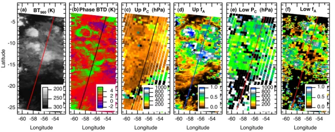
levels. An illustrative (and partial) AIRS granule (defined to be 135 scan lines or 6 min of data) is presented in Fig. 1. Shown is the brightness temperature (BT) at 960 cm−1 10

(BT₉₆₀), a BT difference between 1231 cm−1 and 960 cm−1(BTD) that reveals a sen-sitivity to cloud phase (Nasiri et al., 2007), and PA and fAfor two cloud layers. A wide

variety of structure, including extensive multi-layer clouds, is observed in the P_Aand f_A fields. Figure 1b indicates negative BTDs from 6–8◦S that coincide with Altocumulus (Ac) and Altostratus (As) and higher values of PA and fA, whereas scattered positive

15

BTD are present to the north and south within thinner Cirrus (Ci) layers having lower values of P_A and f_A. The negative and positive BTDs coincide with cloud types con-sistent with liquid water droplets (Ac and As) and ice crystals (Ci), respectively (see Sect. 2.2). For further detail about AIRS cloud retrievals, cloud validation efforts, and cross-comparisons with the Moderate Resolution Imaging Spectroradiometer (MODIS) 20

and Microwave Limb Sounder (MLS), please refer to Susskind et al. (2006), Kahn et al. (2007a,b), Weisz et al. (2007), and references therein.

2.2 CloudSat

CloudSat is a 94 GHz cloud profiling radar providing vertically-resolved information on cloud location, cloud ice and liquid water content (IWC/LWC), precipitation, cloud clas-25

sification, radiative fluxes and heating rates (Stephens et al., 2002). The vertical res-olution is 480 m with 240 m sampling, and the horizontal resres-olution is approximately 1.4 km (cross-track) ×2.5 km (along-track) with sampling roughly every 1 km. Surface

(9)

ACPD

7, 13915–13958, 2007

Full Screen / Esc

EGU

reflection/clutter over most surfaces greatly reduces radar sensitivity in the lowest 3–4 range bins (roughly the lowest km) such that these data are marginally useful in re-lease 3 (R03) (Marchand et al., 2007). An example cross-section of height-resolved reflectivity is shown in Fig. 2a for the same granule introduced in Fig. 1. CloudSat re-veals details in vertical cloud structure that IR sounders are unable to either resolve or 5

sample because the IR signal is emitted by the upper 8–10 or so optical depths of a given cloud profile (Huang et al., 2004).

Range bins with detectable hydrometeors are reported in the 2B-GEOPROF product (Mace et al., 2007). A cloudy range bin is associated with a confidence mask value that ranges from 0–40. Values ≥30 are confidently associated with clouds although values 10

as low as 6 suggest clouds approximately 50% of the time (Marchand et al., 2007). Figure 2b shows the cloud mask for confidence values ≥20. When compared to AIRS cloud fields (Figs. 1 and 2b), P_Aagrees better with CloudSat when f_Ais relatively large. In more tenuous scenes (small f_A) CloudSat infrequently observes clouds. It is unclear if this is a result of clouds with low radar reflectivities (due perhaps to small hydrometeor 15

size), or spurious AIRS cloud retrievals, or just simple mismatches in the sensor time and space sampling. This subject is discussed in Sects. 3 and 4. About 51% of all R03 CloudSat profiles confidently contain at least one range bin with hydrometeors based on three months of data from the Summer of 2006 (Mace et al., 2007). In Release 4 (R04), a combined radar-lidar 2B-GEOPROF product will be produced (Marchand et 20

al., 2007).

The detected clouds in 2B-GEOPROF are assigned cloud types and are reported in the 2B-CLDCLASS product (Wang and Sassen, 2007). Clouds with a confidence mask ≥20 are classified into Ac, As, Cumulonimbus (Cb), Ci, Cumulus (Cu), Nimbo-stratus (Ns), Stratocumulus (Sc), and Stratus (St). The two-dimensional structure and 25

maximum value of cloud reflectivity as well as cloud temperature (based on ECMWF profiles) are combined to identify cloud types. Cloud type frequency and spatial statis-tics are presented in Wang and Sassen (2007) for the initial 6 months of CloudSat observations. In R04 a radar-lidar cloud classification mask will be released. The R03

(10)

ACPD

7, 13915–13958, 2007

Full Screen / Esc

EGU

cloud classification mask is shown in Fig. 2c. Comparison to Fig. 2b strongly suggests bias and variability statistics of AIRS and CloudSat cloud top height differences depend on cloud type. As discussed in the introduction most cloud comparison studies present statistics averaged over multiple cloud types. Thus, cloud type classification is able to provide more relevant and useful satellite-based cloud retrieval comparisons.

5

2.3 CALIPSO

The CALIPSO payload consists of three nadir-viewing instruments: CALIOP, the imag-ing infrared radiometer (IIR), and the wide field camera (WFC) (Winker et al., 2003). This instrument synergy enables the retrieval of a wide range of aerosol and cloud products including (but not limited to): vertically resolved aerosol and cloud layers, ex-10

tinction, optical depth, aerosol and cloud type, cloud water phase, cirrus emissivity, and particle size and shape (Winker et al., 2003; You et al., 2006). We use the Level 1B total attenuated backscatter profiles to illustrate cloud vertical structure, and the 5 km Level 2 cloud feature mask to quantify cloud altitude. The bit-based feature mask indi-cates the presence of cloud and aerosol features (layers) and an associated top and 15

base for each feature detected; up to 10 features are reported for cloud (8 for aerosol). Presently, the publicly released feature mask does not discriminate between cloud and aerosol types although type discrimination is planned for a future release. Relatively weak backscatter for tenuous aerosol and cloud approaches the limits of feature detec-tion with CALIOP, thus varying degrees of horizontal averaging is performed to reduce 20

noise and reveal tenuous features, reported at 333 m, 1, 5, 20, or 80 km depending on the feature. The vertical resolution is 30 m from the surface to 8.2 km; higher than 8.2 km it is 60 m (Vaughan et al., 2005).

2.4 An illustrative cloudy snapshot

The CALIOP 532 nm total attenuated backscatter and 5 km cloud feature mask is 25

(11)

ACPD

7, 13915–13958, 2007

Full Screen / Esc

EGU

cloudiness that have been previously reported are seen in Fig. 2 (Comstock et al., 2002; McGill et al., 2004). When CloudSat (the radar) and CALIOP (the lidar) both detect clouds (6–15◦S), the lidar observes higher cloud tops than the radar. This dif-ference is expected because lidar is more sensitive to small hydrometeors than radar; small ice crystals and water droplets are ubiquitous near cloud tops. The radar pen-5

etrates to the surface through nearly all clouds except for those with significant pre-cipitation (e.g., Cb) unlike most lidars, which generally saturate at optical depth values not much greater than 3 (Comstock et al., 2002). Similarly, the lidar detects exten-sive thin cirrus from 4–6◦S and 15–25◦S that the radar misses. Figure 2b shows that AIRS-derived cloud tops follow the radar more closely than the lidar when thick clouds 10

occur below tenuous clouds (Baum and Wielicki 1994; Weisz et al., 2007). AIRS de-tects much of the thin Ci observed by the lidar only and generally places the upper layer (Z_AU) in the middle or lower portions of the Ci layers (Holz et al., 2006). In some two-layered cloud systems (e.g., Ci, Cu, and Ns from 14–17◦S) AIRS retrieves realistic ZA values for both layers. In more complicated multi-layer cloud structures (e.g., Ac,

15

As, Ns, and Ci detected by the lidar only from 6–10◦S) locating the two dominant cloud tops is problematic. Furthermore, in areas of thick and/or precipitating cloud (e.g., Cb from 11–14◦S), AIRS “retrieves” a lower layer (ZAL) within the cloud at a depth beyond

the expected range of sensitivity for IR sounders. In summary, the cloudy snapshot in Fig. 2 illustrates CloudSat’s ability to profile thick and multi-layered cloud structure, 20

CALIPSO’s ability to accurately determine cloud top boundaries and profile thin clouds, and reveals strengths and weaknesses of IR-based cloud top height retrievals.

3 AIRS, CloudSat and CALIPSO cloud frequency

3.1 Methodology

In this Sect. the comparison approach between AIRS, CloudSat and CALIPSO is out-25

(12)

ACPD

7, 13915–13958, 2007

Full Screen / Esc

EGU

resolutions suggest the results may be sensitive to the treatment of spatial variabil-ity of CloudSat and CALIPSO within the AIRS FOV. Results by Kahn et al. (2007a) (their Table 1) demonstrate a variation in bias of 0.5–1.5 km and variability of 0.3– 0.7 km from using different spatial and temporal averaging approaches between ZAand

surface-based lidar and radar at the Atmospheric Radiation Measurement (ARM) pro-5

gram Manus and Nauru Island sites. Different temporal averages of ARM data (used to replicate the AIRS spatial scale) show similar (smaller) sensitivity for thin (thick) clouds when compared to the sensitivity from different spatial averaging approaches (Kahn et al., 2007a).

Clear sky and cloud frequency statistics for the three instrument platforms are shown 10

in Table 2. CloudSat reports the smallest frequency of clouds whereas AIRS demon-strates the greatest. That AIRS detects more clouds than CALIPSO is an indication of (1) some false cloud detections by AIRS, (2) missed clouds by CALIPSO, or (3) increases in FOV size lead to increases in perceived cloud frequency within some spa-tially heterogeneous cloud fields. Furthermore, a sensitivity of a few percent in AIRS 15

frequency depends on the inclusion of the smallest values of fA. CALIPSO cloud

fre-quency statistics may depend on the resolution of the feature mask (333 m, 1 km, and 5 km) but are not explored here.

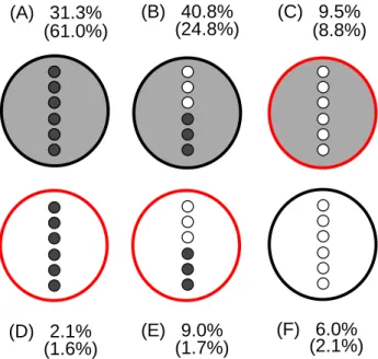
To address the relative frequency of false and positive cloud detections, six general scenarios of coincidence are defined in Fig. 3. The frequency of occurrence for each 20

scenario is shown, which account for heterogeneous and homogeneous cloud fields within an AIRS FOV at any altitude in the vertical column. “False” (scenario C) or “failed” (scenarios D and E) cloud detections occur approximately 20.6% (12.1%) of the time for CloudSat (CALIPSO) comparisons. Some cases are explained by the insensitivity of CloudSat to thin Ci (Scenario C) and the inability of AIRS to detect 25

some low clouds such as Sc and Cu (Scenarios D and E), while others are explained by partial cloud adjacent to the CloudSat/CALIPSO ground track within the AIRS FOV (Scenario C; e.g., Kahn et al., 2005), co-registration/collocation uncertainties (e.g., Kahn et al., 2007b), and other factors. With regard to thin Ci, the CALIPSO comparison

(13)

ACPD

7, 13915–13958, 2007

Full Screen / Esc

EGU

in Scenario C demonstrates a significant portion of either false AIRS detection (see Sect. 4.2) or clouds located outside of the CALIPSO ground track. In Scenarios D and E, many of these cases are thin Ci detected by CALIPSO that are below the detection limit of AIRS. Further analysis using (for instance) MODIS radiances is required to quantify the relative contributions to false and failed AIRS detection frequency.

5

The frequency of each cloud type detected within an AIRS FOV and the percent-age of homogeneous AIRS FOVs (where only one type occurs) are shown in Table 3. For AIRS FOVs that contain As, Cb, Ci and Ns a majority is homogeneous; in con-trast Ac, Cu, and Sc are substantially more heterogeneous. Cloud profiles with verti-cally heterogeneous cloud types will be explored upon release of the combined Cloud-10

Sat/CALIPSO cloud type mask and are not presented here.

3.2 A global five-day climatology

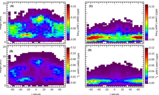
Figure 4 shows AIRS zonally averaged cloud frequency and fA (defined in Sect. 2.1)

from 70◦S–70◦N illustrating the realism of AIRS cloud height (Z_A), amount (f_A), and frequency. Cloud “frequency” is defined as the percentage of AIRS FOVs with non-15

zero fA. In the case of Fig. 4, cloud frequency is partitioned into vertical bins, which

sum to the values shown in Fig. 5. The evaluation of retrievals of Z_A and f_A and their discrepancies are more problematic in Polar latitudes and will be presented elsewhere. Figures 4a and 4b (4c and 4d) illustrate cloud frequency and fA for the upper (lower)

layer, respectively. Familiar global- and regional-scale cloud distributions are revealed. 20

High cloudiness is most frequent in the tropical upper troposphere and mid-latitude storm tracks, whereas low cloud occurs within the subtropics extending to the high latitudes. Furthermore, minima in cloud frequency and amount are observed in the subtropical middle and upper troposphere. These patterns are qualitatively consistent with other climatologies (Rossow and Schiffer 1999; Wylie et al., 1999; Thomas et al., 25

2004).

Zonally averaged cloud frequency and f_Aare shown in Figs. 5a and 5b, respectively. Two minimum values of fA(0.0 and 0.01) used to define cloud in a frequency-based

(14)

cli-ACPD

7, 13915–13958, 2007

Full Screen / Esc

EGU

matology (Fig. 4) illustrate the sensitivity to potentially spurious cloud. Cloud frequency is 5–15% smaller (depending on latitude) using fAU<0.01 for the upper layer, however,

the corresponding change for fAL is only 1–2%. Zonally averaged fA is lower with a

global mean of ∼0.4 for the sum of both layers, consistent with observations from the High Resolution Infrared Radiation Sounder (HIRS) (Wylie et al., 1999). We note that 5

fractional global cloud cover is substantially larger than 0.4, and fA includes the effect

of cloud emissivity. Since many clouds do not radiate as black bodies, the average of fAis expected to be less than the true cloud fraction (or frequency).

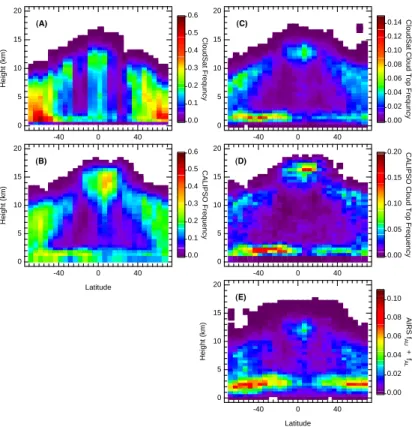
Zonally averaged cloud climatologies for collocated AIRS, CloudSat, and CALIPSO observations are illustrated in Fig. 6. The cloud distribution in Fig. 6 is not represen-10

tative of any particular season or month (Table 1). CloudSat cloud frequency for mask values ≥40 is shown in Fig. 6a. The radar penetrates through nearly all clouds and high frequencies are present throughout the tropical column with the peak from 10– 13 km. However, a climatology like that shown in Fig. 6a is not directly comparable to one derived from AIRS. A climatology of CloudSat-observed cloud tops using the high-15

est cloudy range bin within a given vertical profile is presented in Fig. 6c. The cloud top climatology compares much more favorably with AIRS (Fig. 6e) as expected in terms of zonally-averaged spatial patterns and the magnitude of cloud frequency since AIRS does not sample the full vertical structure of a given cloudy column. Likewise, CALIPSO cloud frequency derived from the 5 km feature mask is shown in Fig. 6b, 20

and the cloud top climatology is shown in Fig. 6d. As with CloudSat, the CALIPSO cloud top climatology qualitatively agrees more favorably with AIRS, although height and sampling biases are apparent from inspection of the frequency patterns with re-spect to height and latitude, these will be explored in more detail in Sect. 4.

There are several additional notable features between AIRS and CloudSat/CALIPSO 25

shown in Fig. 6. First, the peak frequency in the tropical upper troposphere is zonally offset between AIRS and CloudSat by ∼5◦. At least two explanations are possible: (1) the cloud types AIRS and the radar are most sensitive to are not uniformly distributed (i.e., Ci versus Cb) introducing a zonally-dependent sampling bias, and (2) precipitating

(15)

ACPD

7, 13915–13958, 2007

Full Screen / Esc

EGU

clouds occasionally produce ZA retrievals too low in the troposphere with erroneously

low values of f_A(Kahn et al., 2007a). Second, AIRS retrieves tenuous clouds at higher altitudes than the radar in the subtropical latitudes, suggestive of either sensitivity to thin Ci with small ice particles and/or spurious AIRS retrievals. Third, the radar ob-serves high frequencies of low clouds 1–2 km in height in most latitude bands implying 5

a positive height bias for low clouds sensed by AIRS. Fourth, a second layer within Ns from 2–3 km is frequently observed and is inconsistent with IR sensitivity, to be discussed further in Sect. 4.

Several of the radar-lidar differences that are pointed out in Fig. 2 are also observed in Fig. 6. Cloud tops in the upper troposphere observed by the lidar are higher than 10

the radar by 1–4 km depending on the latitude, and are more vertically extensive than observed by AIRS and the radar. This feature is more expansive from 15◦S–15◦N, whereas the peak frequency is shifted 5◦N (10◦N) relative to AIRS (the radar). The broader zonal extent in the lidar climatology is expected because of high sensitivity to thin Ci. The northward shift is consistent with vertically thick and tenuous Ci layers per-15

sisting along the edge of the ITCZ allowing the lidar to detect higher cloud frequencies at lower altitude bins. The lower frequency of lidar-detected clouds from 5◦S–5◦N is a result of sampling biases. At this latitude, clouds are more frequently opaque and precipitating and the lidar observations are restricted to a narrow vertical range re-sulting in fewer detected clouds. Furthermore, the lidar and radar (Figs. 6a and 6b) 20

observe low clouds across most latitudes, however, the radar observes more in the ITCZ and less in the Northern Hemisphere (NH) subtropics than the lidar. The low cloud frequency differences are likely a result from a combination of sampling biases (e.g., upper cloud layers obscuring the lidar’s view of low cloud, the insensitivity of radar to smaller droplets, etc.), and CloudSat’s limitations in the lowest 1.0–1.25 km in R03. 25

Lastly, the frequency minima within subtropical gyres in Fig. 6a extend more poleward into the midlatitudes in Fig. 6b, consistent with the high opacity of clouds in the storm tracks.

(16)

ACPD

7, 13915–13958, 2007

Full Screen / Esc

EGU 4 Height differences partitioned by cloud type

While AIRS estimates up to two cloud layers, the vertical structure cannot be profiled in the manner of a radar or lidar, making comparisons less straightforward than some other studies (Mace et al., 1998; Miller et al., 1999). In this Sect. 4, coincident cloud top height observations between AIRS, CloudSat, and CALIPSO are differenced to quan-5

tify the precision of ZA as a function of fA and cloud type. The resolution of CloudSat

and CALIPSO is not degraded to AIRS, instead each CloudSat and CALIPSO profile is compared to the nearest AIRS retrieval. Random sampling of one CloudSat pro-file per AIRS FOV demonstrates that the bias and variability are within ±0.1–0.3 km for the approach taken in this Sect. 4. Furthermore, we show that biases and vari-10

ability in cloud top differences among different cloud types are several factors larger than those introduced from choosing a particular averaging methodology (Kahn et al., 2007a). More importantly, we will show that the differences among the different cloud types are several factors larger than biases and variability introduced by the choice of sampling strategy. Approximately 45–50 CloudSat profiles (9–10 CALIPSO) coincide 15

with the AIRS FOV. A “nearest neighbor” collocation approach is applied using lati-tude/longitude pairs. The gap between AIRS nadir view and CloudSat and CALIPSO depends on latitude. As a result, an AIRS FOV occasionally contains less than 45–50 CloudSat and 9–10 CALIPSO match-ups since the index of the collocated footprint is not constant with successive scan lines. Fields of fAare averaged to the resolution of

20

ZA. Additional challenges of collocating multiple satellite measurements are addressed

further in Kahn et al. (2007b).

4.1 CloudSat–AIRS

Globally averaged differences of AIRS upper (ZAU) and lower (ZAL) cloud layers with

radar-derived cloud top height (ZCS) are shown in Fig. 7. About 72.1% of AIRS FOVs

25

are comparable to CloudSat, following scenarios A and B presented in Fig. 3; the remaining FOVs are clear or represent false or failed detections, which encompass

(17)

ACPD

7, 13915–13958, 2007

Full Screen / Esc

EGU

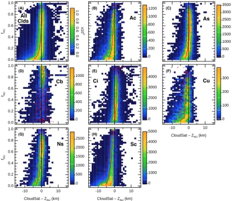
several possibilities (see Sect. 3). The Z_CS is the highest altitude range bin with a confidence mask ≥20; no other cloud layer detected by the radar is used in the com-parison, even in the presence of additional layers. The cloud type associated with the highest range bin classifies the comparisons by cloud type. As discussed in Sect. 3, a histogram approach like that taken by Kahn et al. (2007a) to account for multiple radar-5

derived cloud layers, changes the biases and variability by a smaller amount than those found between different cloud types.

Figures 7a and 7b show differences of ZCS–ZAU ≡ ∆ZU and ZCS–ZAL ≡ ∆ZL,

re-spectively, as a function of fA averaged over all cloud types. The variability is greater

(especially for ∆ZU>0) if the confidence mask is relaxed to values less than 20 (not

10

shown). Figure 7a shows that ∆ZU is a strong (weak) function of fAU<0.2 (fAU>0.2).

The mean bias (solid red line) is −1.0 to −4.0 km for fAU<0.2, increasing to 0.5 km as

f_AU approaches 1.0. Likewise, the variability (dashed red lines) ranges from ±3.5 km for f_AU∼0.01 to ±1.25 km for f_AU∼1.0. There are two contributing factors to the nega-tive bias for fA<0.2: (1) the radar is insensitive to thin and tenuous Ci layers that AIRS

15

detects above lower cloud layers that the radar detects, and (2) some of the small fAU

retrievals are spurious. In Fig. 7b, two broad clusters are suggested for ∆ZL. As fAL

increases, ∆ZL decreases for the cluster with smaller fAL because the lower layer

be-comes the dominant cloud layer. The cluster with higher fALis centered near ∆ZL∼0 km

and is independent of f_AL. This second cluster suggests that AIRS retrieves a quantita-20

tively meaningful lower cloud layer. We will show that the second cluster is associated with particular cloud types.

The results in Fig. 7a are partitioned into individual cloud types using the 2B-CLDCLASS product and are shown in Fig. 8. Several differences of ∆ZU among the

assorted cloud types are observed. First, the negative bias for low fAU in Fig. 7a is

25

primarily due to Sc (the count in Fig. 8h exceeds Figs. 8b–8g), with additional contri-butions from Ac, Cu, and Ns. For these cases the radar detects low or middle clouds while ZAU is located at a higher altitude. Some ZAU are physically plausible (e.g., thin

(18)

ACPD

7, 13915–13958, 2007

Full Screen / Esc

EGU

discussed in Sect. 4.2). Second, the magnitude of f_AUfor individual cloud types is qual-itatively consistent with expectations. For instance, Cb is dominated by fAU>0.8 (low

values occur for partial coverage in the AIRS FOV), Ci is 0.05< fAU<0.4, and Ns is in

between Cb and Ci with 0.5<f_AU<0.9. Few cases of Ns with f_AU>0.9 are observed be-cause non-zero fAL several km below the Ns cloud top is frequently retrieved (fAL+fAU

5

typically sum to 1.0); a similar tendency is also observed within some Cb as well (see Fig. 2). Ac has a lower range of f_AU compared to As, consistent with the classification used in Rossow and Schiffer (1999) and the increased heterogeneity of Ac (Table 3).

Third, both bias and variability strongly depend on cloud type. Sc and Cu have neg-ative ∆ZU, consistent with the high height biases shown for low clouds in Fig. 6. Cb

10

and Ci (and As and Ns for higher values of f_AU) have positive biases of ∆ZU. Holz

et al. (2006) showed that Ci cloud top retrievals derived from IR measurements are frequently placed 1–2 km or more below the physical cloud top. Likewise, Sherwood et al. (2004) showed that height differences derived from geostationary imagery and coincident lidar are 1–2 km even within highly opaque cloud tops. The variability in 15

bias decreases as fAU increases for all cloud types except Ci, which remains

some-what constant with f_AU. The variability is smallest for As, Ci, and Ns (for f_AU>0.5) and largest for Cb (fAU<0.6), Cu (fAU<0.4), and Sc (fAU<0.4). Furthermore, As shows less

variability than Ac. Therefore, more heterogeneous clouds (see Table 3) tend to have larger variability in ∆ZU.

20

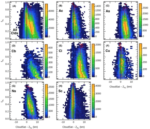
Figure 9 shows the results for ∆ZL. The cluster at small fAL is dominated by As, Cb,

Ci, and Ns. Whether ZAL is a physically reasonable second cloud layer, or a

conse-quence of retrieval algorithm limitations, it is expected that vertical profiles of IWP de-rived from the radar will provide further insight on ZAL. In R03, CloudSat IWP retrievals

in thick and/or precipitating clouds are not reported which hinders the exploration of 25

Z_ALwithin Cb and Ns; however, an improved retrieval is anticipated for the R04 release (2B-CWC-RO R03 data quality statement at http://www.cloudsat.cira.colostate.edu). Sc clouds dominate the cluster with high fAL (see the high count in Fig. 9h) with

(19)

ACPD

7, 13915–13958, 2007

Full Screen / Esc

EGU

liquid water clouds. For Ns clouds, the bias in Z_AL is lower as f_AL increases, resulting in two cloud layers in close vertical proximity when f_AL is large. Despite the complexity in the interpretation of the observed two-layer cloud fields, AIRS is shown to possess skill in detecting and assigning an altitude to low cloud layers.

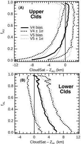
Figure 10 shows mean bias and variability statistics for V4 and V5 AIRS retrievals, 5

and the results for V5 are summarized in Table 4. In Fig. 10a, the bias is substantially smaller for fAU<0.1 and fAU>0.6 in V5. This demonstrates that improvements to cloud

retrievals were made for V5. The larger negative bias for f_AU<0.1 in V4 was primarily a result of poorer retrievals in Ac and Ci (not shown). The larger positive bias in V4 for fAU>0.6 was a result of poorer retrievals in As and Ns, and to a lesser extent, Ci

10

and Cu (not shown). However, in the case of Sc, the V5 bias is larger by 0.25–0.5 km depending on the magnitude of fAU. Differences in day-night and land-ocean biases

and variability were explored. Between day and night, as well as between land and ocean, these differences are not qualitatively significant and are several factors smaller than the differences between V4 and V5 (not shown).

15

4.2 CALIPSO–AIRS

Given the known differences in lidar and radar sensitivity, ZA and lidar-derived cloud

top height (Z_CAL) differences (∆ZCAL) have the potential to be significantly different

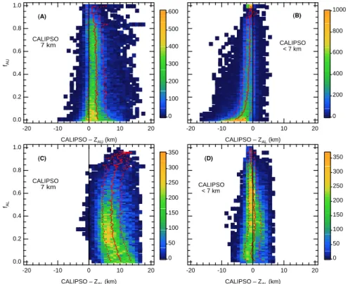
than demonstrated in Sect. 4.1 with the radar. However, Fig. 11 reveals qualitatively similar distributions compared to Fig. 7. The sum of Figs. 11a and 11b (11c and 11d) 20

is analogous to Fig 7a (7b). Clouds are partitioned into two categories with Z_CAL<7 km and ZCAL ≥7 km. About 85.8% of AIRS FOVs are comparable to CALIPSO, following

scenarios A and B presented in Fig. 3; as discussed in Sect. 3 the remaining FOVs are clear or represent false or failed detections. In Fig. 11a, the bias of ∆ZCAL is 1–3 km

with high values for small fAU. The variability is relatively large for small fAU with most

25

of the scatter skewed towards ZCAL>0. This reaffirms the sensitivity of lidar to tenuous

clouds and the tendency for IR-derived cloud tops to be located within the middle or lower portions of Ci layers (Holz et al., 2006).

(20)

ACPD

7, 13915–13958, 2007

Full Screen / Esc

EGU

Differences between Figs. 7a and 11 reveal the following about the lidar–AIRS com-parisons in Fig. 11b: (1) the negative bias for small fAU is greater by 2 km, (2) the

variability is smaller by 0.5–1.0 km, and (3) the largest negative biases are limited to a smaller range of f_AU. The radar’s insensitivity to small hydrometeors is consistent with (3). Another implication of (3) is that ZAU is “reasonable” (although biased in altitude)

5

for many tenuous Ci. This is also suggested by (2) since slightly lower variability is observed with the lidar comparisons, which are more accurate observations of “true” cloud top boundary than radar. Both (1) and (3) suggest many spurious cloud retrievals in the upper troposphere for fAU<0.02. However, the percentage of spurious retrievals

is variable and generally decreases as f_AU increases and are not necessarily restricted 10

to f_A<0.02. The likelihood is small that heterogeneous AIRS FOVs explain a signifi-cant portion of the large negative bias for fAL<0.02 since sub-pixel heterogeneity tends

to increase variability, not necessarily bias (Kahn et al., 2007b). In Fig. 11b, the bias in ∆ZCAL ranges from −2 to −0.5 km as fAU increases from 0.2 to 1.0, whereas the

variability is somewhat smaller than ∆ZU in Fig. 7a. Overall, ZAshows positive height

15

biases for low clouds and negative height biases for high clouds relative to the radar and lidar (although the negative bias for high clouds is larger in the lidar comparisons and smaller for low clouds).

Figures 11c and 11d reveal a tendency for two height clusters as with Fig. 7b. In Fig. 11c (Z_CAL ≥7 km), Z_ALis consistently several km below cloud top, consistent within 20

As, Cb, Ci, and Ns shown in Fig. 9. In Fig. 11d (ZCAL<7 km), ZAL is roughly equal to

ZCALover the range of fAL, which resembles the second cluster in Fig. 7b. Since cloud

classification is not applied in the lidar comparisons, certain cloud types cannot be shown to explain particular height biases. However, Fig. 11d is consistent with Cu and Sc shown in Fig. 9, which implies (like the radar) that ZALis skillful in retrieving a lower

25

layer. The ranges of bias and variability for V5 are summarized in Table 5. As with the CloudSat comparisons, a reduction in negative bias is seen in V5 for tenuous clouds, and day/night and land/ocean differences in bias and variability are much smaller than V4 and V5 differences (not shown).

(21)

ACPD

7, 13915–13958, 2007

Full Screen / Esc

EGU

4.3 Changes in V5 AIRS retrievals and impacts on clouds

Some of the algorithm changes to V5 have the potential to impact cloud retrievals, which include: limiting channel selection for cloud clearing and cloud retrieval to 665– 811 cm−1, treating CO2 as a global and time-dependent constant, updating

spectro-scopic parameters like O3 and HNO3 that affect transmittance in the cloud clearing

5

channels, changing the approach to the downwelling IR radiance term, reducing the number of cloud height retrieval iterations during cloud clearing from 4 to 3, removing the ad hoc error term that impacts the damping parameters for cloud height retrievals (Susskind et al., 2003), and changing the basis of the empirical bias adjustment. The empirical bias correction in V4 used ECMWF analysis fields and in V5 the correction 10

was derived from radiosondes launched during AIRS overpasses that coincided with intensive fields campaigns (Tobin et al., 2006).

The adjustments in the channel list were motivated in large part to eliminate window channels that have large contributions of radiance from the surface. Retrieval yield and precision over surfaces with large spectral emissivity features were improved, but 15

the sensitivity to low clouds was reduced, including oceanic stratus. Thus, the sample size of AIRS and CloudSat comparisons for Sc clouds was smaller from V4 to V5. For instance, the frequency of occurrence of Sc within the dominant subtropical subsidence regions has decreased by as much as 10–20%. The comparisons presented here only consider cases when AIRS and CloudSat/CALIPSO simultaneously observe cloud; it 20

should be emphasized that the V4/V5 differences in Fig. 10 do not include observations when one of the instruments and/or data versions does not sense clouds.

CO2 was assumed to be globally constant at 370 ppm in V4. However, in V5 the

treatment of CO2 was changed to a globally constant linear trend that increases as

a function of time, but is without seasonal or latitudinal variation. In the case of high 25

clouds, sensitivity tests have shown that thin cloud frequency is impacted for changes of 5–10 ppm, typical for regional and seasonal variability, while very little change in fAis

(22)

ACPD

7, 13915–13958, 2007

Full Screen / Esc

EGU

(disappearance) of spurious (physically reasonable) Ci is observed when CO₂ levels are assumed to be too low (high) in the forward model (Hearty et al., 2006). In practice, many thin Ci are placed near the tropopause in otherwise clear sky in retrieved cloud fields. Regarding middle and low clouds, significant changes are observed in f_A, not only the frequency, in the CO2sensitivity tests (Hearty et al., 2006). This demonstrates

5

the need for a more realistic estimate of CO2in the forward model and suggests the

po-tential utility of a simultaneous CO₂retrieval (Chahine et al., 2006) to more accurately retrieve cloud amount and height.

Since the AIRS cloud retrieval steps are initialized with two cloud layers (350 and 850 hPa with f_A of 0.167 and 0.333, respectively), the cloud-clearing algorithm must 10

iteratively “remove” cloud to produce cloud-cleared radiances for downstream retrievals of atmospheric and surface quantities. In a regularized algorithm like that discussed in Susskind et al. (2003), residual f_A may be present in clear scenes because the effectiveness of cloud clearing is limited (in part) by the magnitude of noise in the observed radiances. Thus, small amounts of residual cloud may remain for some clear 15

FOVs. Lastly, global-scale trends of cloud frequency in V5 are greatly reduced over V4 (T. Hearty, personal communication), although the lack of seasonal and latitudinal variability in CO2 likely creates regionally dependent biases in cloud frequency since

cloud type and frequency are not distributed uniformly around the globe (e.g., Rossow and Schiffer 1999; Wylie et al., 1999). Both CALIPSO and CloudSat will continue to 20

play important roles in ongoing assessments of AIRS reprocessing efforts.

5 Conclusions

The precision of cloud height derived from the Atmospheric Infrared Sounder (AIRS), located on EOS Aqua, is explored and quantified for a five-day set of observations. Coincident profiles of vertical cloud structure by CloudSat, a 94 GHz profiling radar, 25

and the Cloud-Aerosol Lidar and Infrared Pathfinder Satellite Observation (CALIPSO) determine the precision of AIRS-derived clouds in a wide variety of geophysical

(23)

condi-ACPD

7, 13915–13958, 2007

Full Screen / Esc

EGU

tions. By fitting simulated and observed spectral radiances, the AIRS retrieval algorithm derives up to two layers of cloud height (ZA) and effective cloud fraction (fA).

Compar-isons are shown for both cloud layers and the entire range of fA. The cloud confidence

and classification masks reported by CloudSat determine cloud occurrence and height and allow the comparisons to be partitioned by cloud type. The 5 km cloud feature 5

mask from CALIPSO is used for the same five-day set of collocated observations. The CloudSat–AIRS biases and variability strongly depend on cloud type, Z_A and fA. Using Version 5 (V5) AIRS retrievals, the cloud top biases range from −4.3 to

0.5 km±1.2 to 3.6 km, depending on fA and cloud type. Large negative biases occur

for the smallest values of f_Aand small positive biases for large f_A. Likewise, the largest 10

variability occurs for the smallest f_A and the smallest variability occurs for the largest values of fA. The upper cloud layer has the highest sensitivity to Altocumulus,

Alto-stratus, Cirrus, Cumulonimbus, and Nimbostratus cloud types and the lower layer to Cumulus and Stratocumulus. The bias and variability for individual cloud types vary widely, but almost all cloud types show reductions in biases and variability with in-15

creasing fA. Furthermore, a tendency for high (low) clouds to be biased low (high) in

height is shown. Frequently, two layers of Z_A are retrieved within Nimbostratus, and to a lesser degree, Cumulonimbus. The lower layer is not necessarily consistent with a physically plausible lower cloud layer. Some cloud types like thin Cirrus, Cumulus, and Stratocumulus are very challenging to characterize with IR measurements. The re-20

sults presented herein suggest that AIRS has skill in detecting and assigning cloud top heights to difficult cloud types. For instance, the bias and variability of Cirrus, Cumu-lus, and Stratocumulus are 0.2 to 1.5±1.1–2.8 km, −0.3 to 1.5±0.3–2.2 km, and −1.3 to −0.3±0.4–1.7 km, respectively. However, AIRS V5 detects a smaller percentage of Sc fields in and around the major oceanic Stratus regions in the subtropics compared 25

to V4.

CALIPSO–AIRS differences qualitatively agree with those from the CloudSat–AIRS comparisons. For CALIPSO cloud tops ≥7 km and <7 km, the biases and variability are 0.6–3.0±1.2–3.6 km, and −5.8 to −0.2±0.5–2.7 km, respectively, with the largest

(24)

ACPD

7, 13915–13958, 2007

Full Screen / Esc

EGU

biases and variability for the smallest values of f_A. The tendency for high clouds to have low Z_Abiases is increased using CALIPSO (rather than CloudSat), consistent with the lidar’s increased sensitivity over the radar to small particles in tenuous cloud top boundaries. Likewise, the high ZAbiases for low clouds are reduced in magnitude. The

large negative Z_Abiases in the CloudSat comparisons for low values of f_Aare increased 5

(decreased) in the CALIPSO comparisons for clouds <7 km (>7 km) in height. This demonstrates that ZA is more precise for thin Cirrus than implied by the CloudSat

comparisons alone. However, there are instances when CALIPSO does not agree with AIRS thin Ci retrievals, demonstrating the existence of spurious ZA in the upper

troposphere. Significant improvements in the AIRS V5 operational retrieval algorithm 10

are demonstrated. Some of the algorithm changes made to V5 are highlighted, and those that could have impacted cloud retrievals are discussed.

In summary, we have demonstrated the utility of CloudSat and CALIPSO to evalu-ate the precision of AIRS cloud retrievals and identified particular cloud types for im-provement. Given the relatively favourable agreement between the active- and passive-15

derived cloud heights, the AIRS swath will be useful to supplement the near-nadir cloud climatology from CloudSat and CALIPSO. Furthermore, since the biases and variabil-ity of AIRS cloud height have been quantified as a function of cloud type, they will help to determine biases in cloud type-dependent microphysical and optical retrievals derived from AIRS radiances and similar IR imagers and sounders because cloud ver-20

tical structure is required for these retrievals. The inter-comparison of these (and other) data sets is a necessary step towards a unified and global view of cloud properties and their validated error estimates.

Acknowledgements. B. H. Kahn was funded by the NASA Post-doctoral Program during this

study and acknowledges the support of the NASA Radiation Sciences Program directed by

25

H. Maring. The authors thank the AIRS, CloudSat, and CALIPSO team members for assis-tance and public release of data products. AIRS data were obtained through the Goddard Earth Sciences Data and Information Services Center (http://daac.gsfc.nasa.gov/). CloudSat data were obtained through the CloudSat Data Processing Center (http://www.cloudsat.cira.

colostate.edu/). CALIPSO data were obtained through the Atmospheric Sciences Data Center

(25)

ACPD

7, 13915–13958, 2007

Full Screen / Esc

EGU

(ASDC) at NASA Langley Research Center (http://eosweb.larc.nasa.gov/). This work was per-formed at the Jet Propulsion Laboratory, California Institute of Technology, under contract with NASA.

References

Aumann, H. H., Chahine, M. T., Gautier, C., Goldberg, M. D., Kalnay, E., McMillan, L. M.,

5

Revercomb, H., Rosenkranz, P. W., Smith, W. L., Staelin, D. H., Strow, L. L., and Susskind, J.: AIRS/AMSU/HSB on the Aqua mission: Design, science objectives, data products, and processing systems, IEEE Trans. Geosci. Remote Sensing, 41, 253–264, 2003.

Baum, B. A. and Wielicki, B. A.: Cirrus cloud retrieval using infrared sounding data: Multilevel cloud errors, J. Appl. Meteor., 33, 107–117, 1994.

10

Chahine, M. T.: Remote sounding of cloudy atmospheres. I. The single cloud layer, J. Atmos. Sci., 31, 233–243, 1974.

Chahine, M. T., Pagano, T. S., Aumann, H. H., et al.: AIRS: Improving weather forecasting and providing new data on greenhouse gases, Bull. Amer. Met. Soc., 87, 911–926, 2006. Chen, T., Rossow, W. B., and Zhang, Y.: Radiative effects of cloud-type variations, J. Climate,

15

13, 264–286, 2000.

Comstock, J. M., Ackerman, T. P., and Mace, G. G.: Ground-based lidar and radar remote sensing of tropical cirrus clouds at Nauru Island: Cloud statistics and radiative impacts, J. Geophys. Res., 107, 4714, doi:10.1029/2002JD002203, 2002.

Fetzer, E. J., Lambrigtsen, B. H., Eldering, A., Aumann, H. H., and Chahine, M. T.:

Bi-20

ases in total precipitable water vapor climatologies from Atmospheric Infrared Sounder and Advanced Microwave Scanning Radiometer, J. Geophys. Res., 111, D09S16, doi:10.1029/2005JD006598, 2006.

Gedzelman, S. D.: Cloud classification before Luke Howard, Bull. Amer. Met. Soc., 70, 381– 395, 1989.

25

Hartmann, D. L., Ockert-Bell, M. E., and Michelsen, M. L.: The effect of cloud type on Earth’s energy balance: Global analysis, J. Climate, 5, 1281–1304, 1992.

Hartmann, D. L., Moy, L. A., and Fu, Q.: Tropical convection and the energy balance at the top of the atmosphere, J. Climate, 14, 4495–4511, 2001.

(26)

ACPD

7, 13915–13958, 2007

Full Screen / Esc

EGU

Hearty, T., Kahn, B. H., and Fishbein, E.: Layer trends in Earth’s cloud cover, Fall Meeting, American Geophysical Union, San Francisco, CA, 2006.

Holz, R. E., Ackerman, S., Antonelli, P., Nagle, F., Knuteson, R. O., McGill, M., Hlavka, D. L., and Hart, W. D.: An improvement to the high spectral resolution CO₂slicing cloud top altitude retrieval, J. Atmos. Oceanic Technol., 23, 653–670, 2006.

5

Houghton, J. T., Ding, Y., Griggs, D. J., et al.: Intergovernmental Panel on Climate Change: Climate Change 2001: The Scientific Basis, 881 pp., Cambridge Univ. Press, New York, 2001.

Huang, H.-L., Yang, P., Wei, H., Baum, B. A., Hu, Y., Antonelli, P., and Ackerman, S. A.: Infer-ence of ice cloud properties from high spectral resolution infrared observations, IEEE Trans

10

Geosci. Remote Sens., 42, 842–853, 2004.

Inoue, T. and Ackerman, S. A.: Radiative effects of various cloud types as classified by the split window technique over the Eastern Sub-tropical Pacific derived from collocated ERBE and AVHRR data, J. Met. Soc. Japan, 80, 1383–1394, 2002.

Jin, Y., Rossow, W. B., and Wylie, D. P.: Comparison of the climatologies of high-level clouds

15

from HIRS and ISCCP, J. Climate, 9, 2850–2879, 1996.

Kahn, B. H., Liou, K.-N., Lee, S.-Y., Fishbein, E. F., DeSouza-Machado, S., Eldering, A., Fetzer, E. J., Hannon, S. E., and Strow, L. L.: Nighttime cirrus detection using Atmospheric Infrared Sounder window channels and total column water vapor, J. Geophys. Res., 110, D07203, doi:10.1029/2004JD005430, 2005.

20

Kahn, B. H., Eldering, A., Braverman, A. J., Fetzer, E. J., Jiang, J. H., Fishbein, E., and Wu, D. L.: Toward the characterization of upper tropospheric clouds using Atmospheric In-frared Sounder and Microwave Limb Sounder observations, J. Geophys. Res., 112, D05202, doi:10.1029/2006JD007336, 2007a.

Kahn, B. H., Fishbein, E., Nasiri, S. L., Eldering, A., Fetzer, E. J., Garay, M. J., and

25

Lee, S.-Y.: The radiative consistency of Atmospheric Infrared Sounder and Moderate Resolution Imaging Spectroradiometer cloud retrievals, J. Geophys. Res., 112, D09201, doi:10.1029/2006JD007486, 2007b.

Klein, S. A. and Hartmann, D. L.: The seasonal cycle of low stratiform clouds, J. Climate, 6, 1587–1606, 1993.

30

Kulawik, S. S., Worden, J., Eldering, A., Bowman, K., Gunson, M., Osterman, G. B., Zhang, L., Clough, S., Shephard, M. W., and Beer, R.: Implementation of cloud retrievals for Tropospheric Emission Spectrometer (TES) atmospheric retrievals: part 1. Description

(27)

ACPD

7, 13915–13958, 2007

Full Screen / Esc

EGU

and characterization of errors on trace gas retrievals, J. Geophys. Res., 111, D24204, doi:10.1029/2005JD006733, 2006.

L’Ecuyer, T. S., Masunaga, H., and Kummerow, C. D.: Variability in the characteristics of precipi-tation systems in the Tropical Pacific. Part II: Implications for atmospheric heating, J. Climate, 19, 1388–1406, 2006.

5

Mace, G. G. and Jakob, C.: Validation of hydrometeor occurrence predicted by the ECMWF model using millimeter wave radar data, Geophys. Res. Lett., 25, 1645–1648, 1998.

Mace, G. G., Marchand, R., Zhang, Q., and Stephens, G.: Global hydrometeor occurrence as observed by CloudSat: Initial observations from Summer 2006, Geophys. Res. Lett., 34, L09808, doi:10.1029/2006GL029017, 2007.

10

Marchand, R., Mace, G. G., Ackerman, T., and Stephens, G.: Hydrometeor detection using CloudSat – An Earth observing 94 GHz cloud radar, accepted, J. Atmos. Ocean. Tech., 2007.

McGill, M. J., Li, L., Hart, W. D., Heymsfield, G. M., Hlavka, D. L., Racette, P. E., Tian, L., Vaughan, M. A., and Winker, D. M.: Combined lidar-radar remote sensing: Initial results from

15

CRYSTAL-FACE, J. Geophys. Res., 109, D07203, doi:10.1029/2003JD004030, 2004. Miller, S. D., Stephens, G. L., and Beljaars, A. C. M.: A validation survey of the ECMWF

prognostic cloud scheme using LITE, Geophys. Res. Lett., 26, 1417–1420, 1999.

Miller, S. D., Stephens, G. L., Drummond, C. K., Heidinger, A. K., and Partain, P. T.: A multi-sensor diagnostic satellite cloud property retrieval scheme, J. Geophys. Res., 105, 19 995–

20

19 971, 2000.

Nasiri, S. L., Kahn, B. H., and Baum, B. A.: Improvement of cloud thermodynamic phase assessment using infrared hyperspectral measurements, Optical Society of America, HISE, Topical Meeting, Santa Fe, New Mexico, February 20–24, 2007.

Parkinson, C. L.: Aqua: An earth-observing satellite mission to examine water and other climate

25

variables, IEEE Transactions on Geoscience and Remote Sensing, 41, 173–183, 2003. Ramanathan, V., Cess, R. D., Harrison, E. F., Minnis, P., Barkstrom, B. R., Ahmad, E., and

Hartmann, D.: Cloud-radiative forcing and climate: Results from the Earth Radiation Budget Experiment, Science, 243, 57–63, 1989.

Remer, L. A., Kaufman, Y. J., Tanr ´e, D., Mattoo, S., Chu, D. A., Martins, J. V., Li, R. R., Ichoku,

30

C., Levy, R. C., Kleidman, R. G., Eck, T. F., Vermote, E., and Holben, B. N.: The MODIS aerosol algorithm, products, and validation, J. Atmos. Sci., 62, 947–973, 2005.

(28)

ACPD

7, 13915–13958, 2007

Full Screen / Esc

EGU

Ruprecht, E., Seze, G., Simmer, C., and Smith, E.: ISCCP cloud algorithm intercomparisons, J. Appl. Meteor. Clim., 24, 877–903, 1985.

Rossow, W. B., Walker, A. W., and Garder, L. C.: Comparison of ISCCP and other cloud amounts, J. Climate, 6, 2394–2418, 1993.

Rossow, W. B. and Schiffer, R.A.: Advances in understanding clouds from ISCCP, Bull. Amer.

5

Met. Soc., 80, 2261–2287, 1999.

Schoeberl, M. R., Douglass, A. R., Hilsenrath, E., Bhartia, P. K., Beer, R., Waters, J. W., Gunson, M. R., Froidevaux, L., Gille, J. C., Barnett, J. J., Levelt, P. F., and DeCola, P.: Overview of the EOS Aura mission, IEEE Trans. Geosci. Remote Sensing, 44, 1066–1074, 2006.

10

Sherwood, S. C., Chae, J.-H., Minnis, P., and McGill, M.: Underestimation of deep convective cloud tops by thermal imagery, Geophys. Res. Lett., 31, L11102, doi:10.1029/2004GL019699, 2004.

Stephens, G. L., Vane, D. G., Boain, R. J., Mace, G. G., Sassen, K., Wang, Z., Illingworth, A. J., O’Connor, E. J., Rossow, W. B., Durden, S. L., Miller, S. D., Austin, R. T., Benedetti, A.,

15

Mitrescu, C., and the CloudSat Science Team: The CloudSat mission and the A-train, Bull. Am. Met. Soc., 83, 1771–1790, 2002.

Stephens, G. L.: Cloud feedbacks in the climate system: A critical review, J. Climate, 18, 237– 273, 2005.

Susskind, J., Barnet, C. D., and Blaisdell, J. M.: Retrieval of atmospheric and surface

param-20

eters from AIRS/AMSU/HSB data in the presence of clouds, IEEE Trans. Geosci. Remote Sens., 41, 390–409, 2003.

Susskind, J., Barnet, C., Blaisdell, J., Iredell, L., Keita, F., Kouvaris, L., Molnar, G., and Chahine, M.: Accuracy of geophysical parameters derived from Atmospheric Infrared Sounder/Advanced Microwave Sounding Unit as a function of fractional cloud cover, J.

Geo-25

phys. Res., 111, D09S17, doi:10.1029/2005JD006272, 2006.

Thomas, S. M., Heidinger, A. K., and Pavolonis, M. J.: Comparison of NOAA’s operational AVHRR-derived cloud amount to other satellite-derived cloud climatologies, J. Climate, 17, 4805–4822, 2004.

Tobin, D. C., Revercomb, H. E., Knuteson, R. O., Lesht, B. L., Strow, L. L., Hannon, S. E., Feltz,

30

W. F., Moy, L. A., Fetzer, E. J., and Cress, T. S.: Atmospheric Radiation Measurement site atmospheric state best estimates for Atmospheric Infrared Sounder temperature and water retrieval validation. J. Geophys. Res., 111, D09S14, doi:10.1029/2005JD006103, 2006.