0044-2275/03/050822-17 DOI 10.1007/s00033-003-3208-z
c
° 2003 Birkh¨auser Verlag, Basel Mathematik und Physik ZAMPZeitschrift f¨ur angewandte
Sharp parameter ranges in the uniform anti-maximum
principle for second-order ordinary differential operators
Wolfgang Reichel
To L.E. Payne on the occasion of his 80th birthday
Abstract. We consider the equation (pu0)0− qu + λwu = f in (0, 1) subject to homogenous boundary conditions at x = 0 and x = 1 , e.g., u0(0) = u0(1) = 0 . Let λ1 be the first eigenvalue of the corresponding Sturm-Liouville problem. If f ≤ 0 but 6≡ 0 then it is known that there exists δ > 0 (independent on f ) such that for λ ∈ (λ1, λ1+δ] any solution u must be negative. This so-called uniform anti-maximum principle (UAMP) goes back to Cl´ement, Peletier [4]. In this paper we establish the sharp values of δ for which (UAMP) holds. The same phenomenon, including sharp values of δ , can be shown for the radially symmetric p -Laplacian on balls and annuli in Rn provided 1 ≤ n < p . The results are illustrated by explicitly computed examples.
Mathematics Subject Classification (2000). Primary: 34B05; Secondary: 35J25
Keywords. Uniform antimaximum principle, SturmLiouville problem, radially symmetric p
-Laplacian
1. Introduction and main results
Let L = aij(x)∂ij2 + bi(x)∂i+ c(x) be a uniformly elliptic operator on a bounded
C2-domain Ω⊂ Rn with continuous coefficients. Consider the boundary value
problem
Lu + λu = f in Ω, ∂νu + bu = 0 on ∂Ω (1)
with a C1-function b ≥ 0 and f ∈ Lq(Ω) , q > n . Let λ
1 denote the first
eigenvalue of L subject to the above boundary condition. Then two important principles hold for solutions u∈ W2,q(Ω) of (1):
Maximum principle (MP): If f ≤ 0 , f < 0 on a set of positive measure and λ < λ1 then u > 0 in Ω .
Anti-maximum principle (AMP): If f ≤ 0 , f < 0 on a set of positive measure
then there exists δ = δ(f ) > 0 such that λ∈ (λ1, λ1+ δ] implies u < 0 in Ω . The (AMP) was discovered by Cl´ement, Peletier [4]. In the same paper a proof
of the well known (MP) is given. In [4] the authors also consider the uniform
anti-maximum principle (UAMP), where the constant δ does not depend on the data f . They showed that (UAMP) holds in dimension n = 1 (and does not hold in
higher dimensions). For example, by computing the Green function G(s, t) for the operator d2/dx2+ λ on the interval (0, 1) with Neumann boundary conditions at x = 0, 1 one finds that G(s, t) < 0 for λ ∈ (0, π2/4] , whereas G(s, t) is
sign-changing for λ > π2/4 . Hence for
u00+ λu = f in (0, 1), u0(0) = u0(1) = 0 (UAMP) holds precisely for λ∈ (0, π2/4] .
Subsequently, both (AMP) and (UAMP) have been extended to linear problems with sign-changing weight by Hess [9] and Godoy et al. [8]. Recently Cl´ement and Sweers [5] found conditions under which (AMP) and (UAMP) hold for higher-order elliptic boundary value problems. For the p -Laplacian div (|∇u|p−2∇u)
Fleckinger et al. [6] showed the (AMP) by a proof different to the one in [4]. Fleckinger and Takaˇc [7] consider (AMP) for p -Laplacian equations, cooperative systems and even Schr¨odinger operators in Rn. For the first time the question of the sharp constant in the (UAMP) for the p -Laplacian on a bounded domain in Rn with 1 ≤ n < p and homogeneous Neumann boundary conditions was
addressed by Arias et al. [1]. Below we will compare our results with the ones in [1].
In this paper we characterize the precise parameter-range of (UAMP) for the problem
(pu0)0− qu + λwu = f in (0, 1), Bu = 0, (2) where Bu is an abbreviation for the boundary condition
(αu + pu0)|x=0= 0, (βu + pu0)|x=1= 0
with constants α, β∈ R . We assume p, q, w, f ∈ C[0, 1] and p, w > 0 in [0, 1] . Solutions are understood such that u, pu0 ∈ C1[0, 1] . To describe our results we use the following notation: let λαβ1 be the first eigenvalue of the Sturm-Liouville problem associated with (2). In this notation λ∞β1 , λα∞1 stands for the first eigenvalue with zero Dirichlet boundary condition at x = 0 , x = 1 , respectively, and unchanged boundary condition at the opposite endpoint, i.e.,
λαβ1 : (αu + pu0)|x=0= 0, (βu + pu0)|x=1= 0,
λ∞β1 : u(0) = 0, (βu + pu0)|x=1= 0,
λα∞
1 : (αu + pu0)|x=0= 0, u(1) = 0.
The corresponding eigenfunctions are denoted by uαβ1 , u∞β1 and uα∞
1 .
Theorem 1. (i) (UAMP) holds for (2) if λ∈ (λαβ1 , min{λ∞β1 , λα∞
1 }] and f ≤ 0 ,
f 6≡ 0 with the conclusion u < 0 in [0, 1] . (ii) For every λ > min{λ∞β1 , λα∞
1 }
Remark. In [4] Cl´ement, Peletier only considered the case α≤ 0 and β ≥ 0 . Our result makes no restriction on the sign of α, β .
An application of (UAMP) to multiple solutions of boundary value problems with discontinuous coefficients is given next. For a function u we use the notation
u+= max{u, 0} and u = u+− u− so that u+, u− are both non-negative.
Corollary 2. Let f ∈ C[0, 1] with f ≤ 0 , f 6≡ 0 and suppose µ < λαβ1 and λαβ1 < ν≤ min{λ∞β1 , λα∞
1 } . Then the boundary value problem
(pu0)0− qu + w(µu+− νu−) = f in (0, 1), Bu = 0 has at least two solutions.
Our second result establishes an analogous theorem for the radially symmetric
p -Laplacian. Recall the definition ∆pv = div (|∇v|p−2∇v) , p > 1 , where v : Ω ⊂
Rn → R . The problem analogous to (1) is
∆pv− q|v|p−2v + λw|v|p−2v = f in Ω, |∂νv|p−2∂νv + b|v|p−2v = 0 on ∂Ω.
For radially-symmetric functions v(x) = u(r) with r =|x| on a ball Ω = B1(0) we find ∆pv(x) = Lpu(r) = r1−n(rn−1|u0|p−2u0)0. We refer to Lp as the radially
symmetric p -Laplacian. Then the boundary value problem corresponding to (2) is given by
Lpu− q|u|p−2u + λw|u|p−2u = f in (0, 1), Bpu = 0, (3) where Bpu = 0 is an abbreviation for the boundary condition
u0(0) = 0, (β|u|p−2u + rn−1|u0|p−2u0)|r=1= 0.
Solutions of (3) are understood such that u, rn−1|u0|p−2u0 ∈ C[0, 1]∩C1[0, 1] . The
nature of the problem is very different in the two cases 1≤ n < p and n ≥ p . We restrict attention to 1 ≤ n < p . In this case (3) together with arbitrary homogenous boundary data at r = 0 and r = 1 is a well defined boundary value problem, cf. Reichel, Walter [11].
Our result for (3) is restricted to the case β = 0 . This has only technical reasons, cf. Lemma 8. We expect the result to hold for arbitrary β ∈ R . We use various first eigenvalues of the Sturm-Liouville problem related to (3). The existence of theses eigenvalues was shown in [11].
λN N
1 : u0(0) = 0, u0(1) = 0,
λDN1 : u(0) = 0, u0(1) = 0,
λN D
1 : u0(0) = 0, u(1) = 0.
Theorem 3. Suppose 1 ≤ n < p and β = 0 . (i) (UAMP) holds for (3) in the class of functions f < 0 in [0, 1] if λ ∈ (λN N
conclusion u < 0 in [0, 1] . (ii) For every λ > min{λDN
1 , λN D1 } there exists a
function f≤ 0 and a sign-changing solution u of (3).
Remarks. (a) The restriction to f < 0 in [0, 1] is again technical, cf. Lemma 8.
We expect the result to hold for f≤ 0 , f 6≡ 0 as in Theorem 1.
(b) The same result holds on an annulus A : {x ∈ Rn : R1 <|x| < R2} with
boundary conditions u0(R1) = u0(R2) = 0 .
Corollary 4. Let f ∈ C[0, 1] with f < 0 in [0, 1] and suppose µ < λN N
1 and
λN N
1 < ν ≤ min{λN D1 , λDN1 } . Then the boundary value problem
Lpu− q|u|p−2u + w|u|p−2(µu+− νu−) = f in (0, 1), u0(0) = u0(1) = 0.
has at least two solutions.
Arias et al. established in [1] sharp intervals for the (UAMP) for the p -Laplacian problem ∆pu + λ|u|p−2u = f (x) in Ω with zero Neumann boundary
data on an arbitrary bounded domain Ω⊂ Rn with 1 ≤ n < p . They showed
that the interval (λ1, ¯λ] with
¯ λ = inf u∈W1,p(Ω) Z Ω|∇u| pdx : Z Ω|u| pdx = 1, u vanishes somewhere in Ω, (4)
is the sharp interval for (UAMP). This is consistent with our results of Theorem 1 and Theorem 3. In fact, Arias et al. show that the minimizer in (4) has exactly one zero in Ω . If compared with our results for ode-operators, one is led to conjecture that the minimizer in (4) attains its zero on ∂Ω . In our case ¯λ then
coincides with an eigenvalue with a Dirichlet boundary condition at one endpoint. It remains open how the sharp result of Arias et al. can be generalized to the
p -Laplacian Neumann boundary value problem ∆pu− q|u|p−2u + λw|u|p−2u = 0
with a potential q .
The proof of (AMP) and (UAMP) given by Cl´ement, Peletier [4] is functional analytic; the one by Arias et al. [1] is variational. On the other hand, the standard proofs of (MP) involve pointwise differential inequalities and are not functional an-alytic. In this paper we prove the sharp (UAMP) again with the help of differential inequalities.
2. Proof of Theorem 1 and Corollary 2
The first lemma reduces the proof of (UAMP) to a more special situation.
Lemma 5. To prove the (UAMP) of Theorem 1 it suffices to prove the following weaker version: if f ∈ C[0, 1] with f < 0 in [0, 1] is such that the solution u of
Proof. Part 1: Suppose (UAMP) of Theorem 1 holds for all f < 0 in [0, 1] with
the (weaker) conclusion u≤ 0 . We show how the full version of (UAMP) follows. Let I = (λαβ1 , min{λ∞β1 , λα∞
1 }] and suppose λ ∈ I . Since no other eigenvalue
λαβi lies in I we can consider the Green-function G(x, y) for the boundary value problem (2), i.e.,
(pG0(x, y))0− qG(x, y) + λwG(x, y) = −δy(x) ∀x, y ∈ (0, 1) with x 6= y,
where differentiation is with respect to x . Moreover G(x, y) as a function of x satisfies the boundary conditions for every fixed y . By approximation of δy(x)
by smooth strictly positive functions and by application of the hypotheses of part 1 we find that G(x, y) ≥ 0 . And since −G(x, y) satisfies a linear differential equation except for x = y we find −G(x, y) > 0 for all x, y ∈ [0, 1] , x 6= y . Once this is established the full version of (UAMP) follows.
Part 2: Now we want to show that it even suffices to consider only those f < 0 in [0, 1] , where the solution u has at most simple isolated zeros. Suppose we know that (UAMP) with conclusion u≤ 0 holds for all f < 0 in [0, 1] such that
u has at most simple isolated zeros. Fix now an arbitrary ˜f ∈ C[0, 1] with ˜f < 0
in [0, 1] and let ˜u be the corresponding solution. Clearly ˜u has isolated zeros.
We need to show ˜u≤ 0 . Suppose a function ψ ∈ C2[0, 1] exists with ψ > 0 in (0, 1) , Bψ = 0 and such that ˜u²= ˜u + ²ψ has at most simple isolated zeros for
all ²∈ (0, ²0) . Let −δ = max[0,1]f < 0 . Then˜
(p˜u0²)0− q˜u²+ λw˜u²= ˜f + ²
³
(pψ0)0− qψ + λwψ ´
≤ −δ/2
provided ² is small enough. By the hypotheses of part 2 we obtain ˜u²≤ 0 and by
taking the limit ²→ 0 we also find ˜u ≤ 0 . Thus, the (UAMP) with conclusion ˜
u≤ 0 holds for all ˜f with ˜f < 0 in [0, 1] .
Part 3: It remains to construct the function ψ used in part 2. If ˜u has
a double zero at x = 0 or x = 1 then ˜u + ²uαβ1 has no zero at x = 0, 1 . Suppose next that ˜u has multiple zeros at 0 < x1 < . . . < xk < 1 . For small
enough η we can achieve that in the interval (xi− η, xi+ η) the function ˜u0 only
vanishes at xi, since xi cannot be an accumulation point of zeros of ˜u0 due to
the assumption ˜f ≤ −δ < 0 . Next we choose the C2-function ψ as shown in Figure 2 with support in [xi− η, xi+ η] . If ²0 is so small that ˜u + ²ψ6= 0 in
[xi− η, xi−η2] and [xi+η2, xi+ η] for ²∈ (0, ²0) then ˜u + ²ψ has only simple
zeros in [xi− η, xi+ η] . This finishes the construction of ψ .
The following transformation is standard for Sturm-Liouville eigenvalue prob-lems. For non-zero right hand sides the proof can be adapted from Coddington, Levinson [3].
Lemma 6 (Pr¨ufer transformation). Let u be a solution of (2) with at most simple
zeros. Then there are C1-functions ρ, φ : [0, 1]→ R with pu0 = ρ cos φ, u = ρ sin φ
x
ix
i+
η2x
i+ η
x
i−
η2x
i− η
1
ψ(x)
Figure 1. Choice of ψand φ(0) ∈ (0, 2π) with cot φ(0) = −α , cot φ(1) = −β . Moreover, ρ > 0 in
[0, 1] , and ρ, φ satisfy φ0 = (−q + λw) sin2φ +1 pcos 2φ−f ρsin φ, (5) ρ0 = ρ ³ (q− λw +1 p) sin φ cos φ ´ + f cos φ. (6)
Remark. Equation (5) shows that φ can cross the lines kπ only from below
with positive slope.
Likewise, the eigenfunctions uα∞
1 , u∞β1 and uαβ1 can be written in
polar-coordinates (φα∞, ρα∞), (φ∞β, ρ∞β) and (φαβ, ραβ) , where we take uα∞
1 , uβ∞1
negative but uαβ1 positive. Hence the angle-functions satisfy φαβ 0 = (−q + λαβ1 w) sin2φαβ+1 pcos 2φαβ, (7) φαβ(0) = π− arccot α, φαβ(1) = π− arccot β, φα∞0 = (−q + λα∞1 w) sin2φα∞+1 pcos 2φα∞, (8) φα∞(0) = 2π− arccot α, φα∞(1) = 2π, φ∞β0 = (−q + λ∞β1 w) sin2φ∞β+1 pcos 2φ∞β, (9) φ∞β(0) = π, φ∞β(1) = 2π− arccot β.
Lemma 7 (Comparison principle). Assume g(x, s) is defined on the set [0, 1]×R and is uniformly Lipschitz-continuous with respect to s on compact subsets of
[0, 1]× R . If the functions φ, ψ are C1-functions on (0, 1] , continuous in [0, 1] with φ(0)≤ ψ(0) and
φ0− g(x, φ) ≤ 0, ψ0− g(x, ψ) ≥ 0 in (0, 1)
then the conclusion φ(x)≤ ψ(x) in [0, 1] holds. Moreover, either φ < ψ in [0, 1] or φ≡ ψ in [0, 1] or there exists x0 ∈ (0, 1) such that φ = ψ on [0, x0] and
φ < ψ on (x0, 1] . The function φ, ψ is called a sub-, supersolution, respectively.
Remark. For a pair of sub-, supersolutions φ, ψ with φ− g(x, φ) ≤ 0, 6≡ 0 the
comparison principle implies φ(1) < ψ(1) . This will be used frequently in the proof of Theorem 1.
Proof. Part 1: On a finite interval [0, 1] the functions φ, ψ attain their values in
the interval [−M, M] . Let L be the Lipschitz constant of g w.r.t. the second variable on the compact set [0, 1]× [−M, M] . The difference ξ = ψ − φ satisfies
ξ0≥ g(x, ψ) − g(x, φ) ≥ −L|ξ| on [0, 1] . This shows that ξe−Lx is increasing on intervals where ξ is negative. Since ξ(0)≥ 0 we get ξ ≥ 0 on [0, 1] .
Part 2: Now that we know ξ = ψ− φ ≥ 0 we find that ξ0 ≥ −Lξ on [0, 1] , i.e. ξeLx is increasing. In particular, if ξ is positive somewhere, then it stays
positive.
Proof of Theorem 1. First we assume λ∈ (λαβ1 , min{λ∞β1 , λα∞
1 }] and show that
the weaker version of (UAMP) from Lemma 5 holds. Let f < 0 in [0, 1] and let
u be a solution of (2) with at most simple zeros. Let φ be the angle-function
of u from Lemma 6. The form of the boundary condition and the assumption of simple zeros excludes the case u(0) = 0 . Thus we are left with the two cases
φ(0)∈ (0, π) or φ(0) ∈ (π, 2π) .
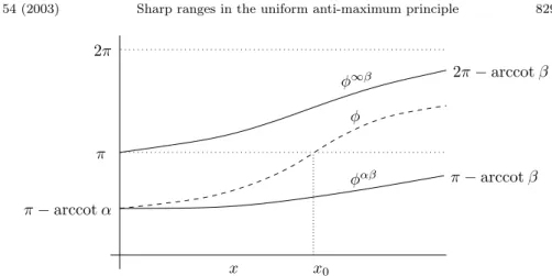
Case 1: φ(0) = π− arccot α ∈ (0, π) . As long as φ attains values in [0, π]
we have φ0 ≥ (−q + λαβ1 w) sin2φ +1pcos2φ . Hence φ is a supersolution to φαβ.
If φ stayed in [0, π] then Lemma 7 would imply π ≥ φ(1) > φαβ(1) , i.e. φ
could not attain the correct boundary condition. Hence φ must attain values in [π, 2π] , i.e. φ(x) > π for x > x0. As long as φ attains values in [π, 2π] we have φ0≤ (−q + λ∞β1 w) sin2φ +1pcos2φ , i.e. φ is a subsolution to φ∞β1 . Hence Lemma 7 applies on [x0, 1] and shows that φ stays below φ∞β. In particular
π ≤ φ(1) < 2π − arccot β . Thus φ cannot attain the prescribed boundary
condition. This contradiction shows that case 1 cannot occur. The situation is depicted in Figure 2.
Case 2: φ(0) = 2π− arccot α ∈ (π, 2π) . Clearly φ(x) stays above π . As long
as φ∈ [π, 2π] we have φ0 ≤ (−q +λα∞
1 w) sin2φ +1pcos2φ , i.e. φ is a subsolution
to φα∞
1 . By Lemma 7 we get π≤ φ ≤ φα∞1 , i.e, φ stays in [π, 2π] which implies
u≤ 0 as claimed. This situation is depicted in Figure 3.
It remains to show that the interval (λαβ1 , min{λ∞β1 , λα∞
1 }] is the largest
pos-sible interval for the (UAMP). We use a result about the following boundary value problem:
(pu0)0− qu + w(µu+− νu−) = 0 in (0, 1), Bu = 0.
A pair of values (µ, ν) is called a Fuˇcik-eigenvalue if the above problem has a non-trivial solution. The set of all Fuˇcik-eigenvalues is called the Fuˇcik-spectrum.
2π π− arccot β 2π− arccot β π π− arccot α φ φ∞β φαβ x x0
Figure 2. φαβ pushes φ above π , φ∞β keeps it below 2π − arccot β
2π 2π− arccot β π x φ 2π− arccot α φα∞
Figure 3. φα∞ keeps φ below 2π
Next to the trivial lines λαβ1 × R and R × λαβ1 the Fuˇcik-spectrum consists of a collection of curves σi+ and σ−i , i = 2, . . . ,∞ , with σi+∩ σ−i ={(λαβi , λαβi )} . The Fuˇcik-eigenfunctions corresponding to σ+i , σ−i have i− 1 zeros in (0, 1) and are positive, negative at 0 , respectively. The main result, which we are using is the asymptotic behaviour of σ2+, σ−2 , as found by Reichel, Walter [11] and Rynne [12]. Let ν+(µ) , ν−(µ) be the parameterizations of σ+2, σ−2 . Then
ν+, ν− are decreasing functions with the following asymptotics: limµ→∞ν+(µ) = λ∞β1 , limµ&λα∞1 ν+(µ) =∞,
limµ→∞ν−(µ) = λα∞
1 , limµ&λ∞β1 ν
−(µ) =∞.
Let λ > min{λ∞β1 , λα∞
1 } . If, e.g., λ > λ∞β1 then let (µ, ν) be a point on σ+2
corresponding Fuˇcik-eigenfunction. Necessarily u is sign-changing and satisfies (pu0)0− qu + λu = (λ − µ)u+− (λ − ν)u−=: f ≤ 0.
Thus (UAMP) does not hold for such a λ . If λ > λα∞
1 then let (µ, ν) be a point
on σ2− with µ > λ and ν < λ , which exists for sufficiently large µ . With f ≤ 0 constructed as above we see the (UAMP) cannot hold for such a λ .
Proof of Corollary 2. The proof is very simple. Let µ < λαβ1 and let f ≤ 0 ,
f 6≡ 0 . Since µ is not an eigenvalue the problem
(pu0)0− qu + µwu = f in (0, 1), Bu = 0
has a unique solution u , which is positive by the maximum principle (MP). Hence it also solves
(pu0)0− qu + w(µu+− νu−) = f in (0, 1), Bu = 0. (10) If λαβ1 < ν≤ min{λ∞β1 , λα∞1 } then for the same reason
(pv0)0− qv + νwv = f in (0, 1), Bv = 0
has a unique solution v , which is negative by the (UAMP) of Theorem 1. Hence it also solves (10).
3. Proof of Theorem 3 and Corollary 4
We rewrite equation (3) as
(rn−1|u0|p−2u0)0− rn−1q|u|p−2u + λrn−1w|u|p−2u = rn−1f in (0, 1).
As before we can reduce the proof of (UAMP) to a simpler situation. However, since there is no p -Laplacian Green function, we need to argue differently.
Lemma 8. To prove the (UAMP) of Theorem 3 is suffices to prove the following weaker version: if f ∈ C[0, 1] with f < 0 in [0, 1] is such that the solution u of
(3) has at most simple isolated zeros then u≤ 0 in [0, 1] .
Remarks. If u satisfies boundary conditions more general than zero Neumann
at r = 0 and r = 1 then we do not know how to reduce the (UAMP) to the case where u has at most simple zeros, cf. part 2 of the proof. Also, we do not know how to relax f < 0 to f ≤ 0 .
Proof. Part 1: Suppose (UAMP) holds for f < 0 in [0, 1] but with the weaker
conclusion u≤ 0 in [0, 1] . So let λ ∈ (λN N
1 , min{λN D1 , λDN1 }] . We want to show
that u ≤ 0 can be strengthened to u < 0 in [0, 1] . Suppose u ≤ 0 has an interior zero at r0∈ (0, 1) and suppose f 6≡ 0 on [0, r0] (a similar proof holds if
f 6≡ 0 on [r0, 1] ). Then λ > R0r0(−Lpu + q|u|p−2u)urn−1dr/
Rr0
0 w|u|prn−1dr .
And since u(r0) = 0 we find that
λ > Rr0 0 (R|u0|p+ q|u|p)rn−1dr r0 0 w|u|prn−1dr ≥ λN D 1 [0, r0]
due to the variational characterization of λN D
1 [0, r0] . Since λN D1 [0, r0] is strictly
decreasing in r0, we find λ > λN D
1 [0, r0] > λN D1 . This contradiction shows that
u cannot have a zero in (0, 1) . A similar argument shows that u cannot have a
zero at r = 0 or r = 1 .
Part 2: Now we show that it suffices to consider those f < 0 in [0, 1] such that the solution u has at most simple isolated zeros. Suppose we know that (UAMP) with conclusion u≤ 0 holds for all f < 0 in [0, 1] such that u has at most simple isolated zeros. Fix now an arbitrary ˜f ∈ C[0, 1] with ˜f < 0 in [0, 1]
and let ˜u be a corresponding solution. Clearly ˜u has isolated zeros. We need
to show ˜u≤ 0 . For sufficiently small ² > 0 the function ˜u² = ˜u + ² has simple
zeros, attains Neumann boundary-conditions at r = 0 and r = 1 and satisfies (rn−1|˜u0²|p−2u˜0²)0− rn−1q|˜u²|p−2u˜²+ λrn−1w|˜u²|p−2u˜²= rn−1f˜²,
where ˜f²→ ˜f uniformly as ²→ 0 , i.e., for sufficiently small ² we have ˜f² < 0
in [0, 1] . By the hypotheses of part 2 we obtain ˜u²≤ 0 and by taking the limit
²→ 0 we also find ˜u ≤ 0 . Thus, the (UAMP) with conclusion ˜u ≤ 0 holds for
˜
f < 0 in [0, 1] .
For a Pr¨ufer-type transformation like in Section 2 we need to suitably generalize the concept of the sine-function. Generalized sine-functions are well studied in the literature, see Lindqvist [10]. The generalized sine-function sinp is first defined
locally as the solution of the differential equation
u0p+ u
p
p− 1 = 1 with u(0) = 0, u
0(0) = 1. (11)
Equation (11) arises as a first integral of (u0(p−1))0 + u(p−1) = 0 . The solution defines the functions Sp(φ) = sinp(φ) as long as it is increasing, i.e. for φ ∈ [0, πp/2] , where πp 2 = Z (p−1)1/p 0 dt 1− tp/(p− 1))1/p = (p− 1)1/p p sin(π/p)π. (12)
Since Sp0(πp/2) = 0 we define Sp on the interval [πp/2, πp] by Sp(φ) = Sp(πp−
φ) , and for φ∈ (πp, 2πp] we put Sp(φ) =−Sp(2πp−φ) and extend Sp as a 2πp
-periodic function on R . In the special case p = 2 , S2(x) = sin x and π2 = π . The following properties of Sp will be frequently used:
Lemma 9. For p > 1 the generalized sine-functions Sp have the properties:
(ii) Sp solves |S0p|p+|Sp|
p
p−1 = 1 on R ,
(iii) For 1 < p≤ 2 the function Sp0 is C1, whereas for p≥ 2 the function Sp0 is 1/(p− 1) -H¨older continuous.
Proofs can be obtained from the results of Lindqvist [10]. We show in Figure 4 the graphs of the function Sp for p = 1.4, 2, 5 . As p → ∞ the function Sp
converges to 1− |x − 1| and as p → 1 it approaches 0 .
–1 –0.5 0 0.5 1 1 2 3 4 5 6 S S S 1.4 2 5 Figure 4. Sp, p = 1.4, 2, 5
With the help of the generalized sine-function we transform any solution of (3) with at most simple zeros into phase-space via generalized polar-coordinates
ρ and φ . This has been done by Reichel, Walter [11] and Brown, Reichel [2] as
follows:
rn−1u0(p−1)= ρSp0(φ)(p−1), u(p−1)= ρSp(φ)(p−1). (13) A calculation using the defining properties of Sp and Sp0 as in (ii) of Lemma 9 leads to the pair of equations:
φ0 = r n−1 p− 1(−q + λw)|Sp(φ)| p+ r1−np−1|S0 p(φ)|p− rn−1f (p− 1)ρSp(φ), (14) ρ0= ρ n³ rn−1(q− λw) + r1−np−1 ´ Sp(φ)(p−1)Sp0(φ) o + rn−1f Sp0(φ). (15) Radially symmetric solutions of (3) satisfy u0(0) = u0(1) = 0 . This amounts to φ(0) = πp/2 mod πp and φ(1) = πp/2 mod πp. The following results show that eigenvalues with arbitrary homogeneous boundary conditions at r = 0 and
r = 1 exist provided 1≤ n < p .
Proposition 10 (Reichel, Walter [11]). Let 1≤ n < p and consider the eigen-value problem
with the boundary conditions
(α1|u|p−2u + α
2rn−1|u0|p−2u0)|r=0 = 0,
(β1|u|p−2u + β2rn−1|u0|p−2u0)|r=1 = 0,
(17)
where α21+α22> 0 , β12+β22> 0 . It has a countable number of simples eigenvalues λ1 < λ2 < . . . , limn→∞λn =∞ , and no other eigenvalues. The corresponding
eigenfunction un has n− 1 simple zeros in (0, 1) .
We denote the first eigenfunction for α1 = β1 = 0 by uN N
1 since it has
vanishing Neumann data at both endpoints. Likewise, if α1 = β2 = 0 we de-note the first eigenfunction by uN D
1 since it has zero Dirichlet data at r = 1 .
Finally, the first eigenfunction corresponding to α2 = β1 = 0 is denoted by
uDN
1 . Each of these three functions can be written in generalized polar
coor-dinates (φN N, ρN N), (φN D, ρN D) and (φDN, ρDN) , where we take uN D
1 , uDN1
negative but uN N
1 positive. Hence the angle-functions satisfy
φN N 0 = r n−1 p− 1(−q + λ N N 1 w)|Sp(φN N)|p+ r 1−n p−1|S0 p(φN N)|p, (18) φN N(0) = πp/2, φN N(1) = πp/2, φN D0 = r n−1 p− 1(−q + λ N D 1 w)|Sp(φN D)|p+ r 1−n p−1|S0 p(φN D)|p, (19) φN D(0) = 3πp/2, φN D(1) = 2πp, φDN 0 = r n−1 p− 1(−q + λ DN 1 w)|Sp(φDN)|p+ r 1−n p−1|S0 p(φDN)|p, (20) φDN(0) = πp, φDN(1) = 3πp/2.
As a basic tool for our analysis we use the following more subtle version of the comparison principle, cf. Lemma 7. Such comparison principles can be found in detail in Walter [13].
Lemma 11 (Generalized comparison principle). Let g(r, s) be defined on the set
[0, 1]× R and suppose it satisfies a generalized local Lipschitz-condition w.r.t. s ,
i.e., for every M > 0 there exists a function h∈ L1(0, 1) such that
|g(r, s1)− g(r, s2)| ≤ h(r)|s1− s2| ∀|s1|, |s2| ≤ M, ∀r ∈ (0, 1).
If the functions φ, ψ are C1-functions on (0, 1] , continuous in [0, 1] with φ(0)≤ ψ(0) and
φ0− g(r, φ) ≤ 0, ψ0− g(r, ψ) ≥ 0 in (0, 1)
then the conclusion φ(r)≤ ψ(r) in [0, 1] holds. Moreover, either φ < ψ in [0, 1] or φ≡ ψ in [0, 1] or there exists r0 ∈ (0, 1) such that φ = ψ on [0, r0] and
Proof. The proof is similar to Lemma 7. The function ξ = ψ− φ satisfies
ξ0≥ g(r, ψ) − g(r, φ) ≥ −h(r)|ξ| on intervals [0, 1] . This shows that ξe−R0rh(t)dt
is increasing on intervals where ξ is negative. Since ξ(0) ≥ 0 we get ξ ≥ 0 on [0, 1] . Once ξ ≥ 0 is known one obtains that ξ0 ≥ −h(r)ξ on [0, 1] , i.e.
ξeR0rh(t)dt is increasing. As before we find that if ξ is positive somewhere, then it stays positive.
Proof of Theorem 3. The proof is very similar to the proof of Theorem 1. In
the φ -equation (14) of the Pr¨ufer-transform the singular function r1−np−1 appears.
This function is in L1(0, 1) precisely for 1 ≤ n < p . Hence we can replace the comparison principle of Lemma 7 by the generalized comparison principle of Lemma 11. Figure 2, Figure 3 used in the proof of Theorem 1 still provide a graphical insight into case 1, case 2, respectively, below. Let f < 0 in [0, 1] and let u be a solution of (3) with at most simple zeros and angle-function φ . We consider two cases: φ(0) = πp/2 or φ(0) = 3πp/2 .
Case 1: φ(0) = πp/2 . As long as φ attains values in [0, πp] we have φ0 ≥
rn−1
p−1(−q + λN N1 w)|Sp(φ)|p + r
1−n
p−1|S0
p(φ)|p, i.e., φ is a supersolution to φN N.
Hence φN N pushes φ above πp, i.e. φ(r) > πp for r > r0. As long as φ
attains values in [πp, 2πp] we have φ0≤ r
n−1 p−1(−q +λDN1 w)|Sp(φ)|p+ r 1−n p−1|S0 p(φ)|p i.e. φ is a subsolution to φDN
1 . Hence πp ≤ φ(1) < 3πp/2 . Thus φ cannot
attain the prescribed boundary condition. This contradiction shows that case 1 cannot occur.
Case 2: φ(0) = 3πp/2 . Clearly φ(r) stays above πp. As long as φ∈ [πp, 2πp]
we have φ0≤ rp−1n−1(−q + λN D1 w)|Sp(φ)|p+ r
1−n
p−1|S0
p(φ)|p, i.e., φ is a subsolution
to φN D
1 . Hence φ stays in [πp, 2πp] as claimed.
Finally we need to show that the interval (λN N
1 , min{λDN1 , λN D1 }] is the largest
possible interval for (UAMP). The corresponding Fuˇcik problem is
Lpu− q|u|p−2u + w|u|p−2(µu+− νu−) = 0∈ (0, 1), u0(0) = u0(1) = 0.
Again the Fuˇcik-spectrum consists of the the trivial lines λN N
1 × R and R ×
λN N
1 and a collection of curves σ+i and σ−i , i = 2, . . . ,∞ with σi+∩ σ−i =
{(λN N
i , λN Ni )} . The Fuˇcik-eigenfunctions corresponding to σi+, σ−i have i− 1
zeros in (0, 1) and are positive, negative at 0 , respectively. By the result of Reichel, Walter [11] the asymptotic behaviour of the descreasing curves σ2+, σ2− is given as follows:
limµ→∞ν+(µ) = λDN1 , limµ&λND1 ν
+(µ) =∞,
limµ→∞ν−(µ) = λN D1 , limµ&λDN1 ν+(µ) =∞.
Just as in Theorem 1 this enables us to shows that (UAMP) cannot hold for
λ > min{λ∞β1 , λα∞
Proof of Corollary 4. Let µ < λN N1 and let f < 0 in [0, 1] . Then
Lpu− q|u|p−2u + µw|u|p−2u = f in (0, 1), u0(0) = u0(1) = 0
has a positive solution u . In fact, u can be obtained as a minimizer of the functional J [u] =R01(|u0|p+ q|u|p− µw|u|p+ pf u)rn−1dr in C1[0, 1] , which is bounded below by the assumption µ < λN N
1 . Since |u| also provides a minimizer,
we may assume u≥ 0 . Hence u solves
Lpu− q|u|p−2u + w|u|p−2(µu+− νu−) = f in (0, 1), u0(0) = u0(1) = 0. (21)
Likewise, if λN N
1 < ν ≤ min{λDN1 , λN D1 } then
Lpu− q|v|p−2v + νw|v|p−2v = f in (0, 1), v0(0) = v0(1) = 0
has a solution v , cf. Reichel, Walter [11], Theorem 3. By the (UAMP) of Theo-rem 3 we find v≤ 0 . Hence v also solves (21).
4. Examples
For three different boundary value problems we determine the optimal parameter ranges for (UAMP) explicitely/numerically.
4.1. The Fourier equation
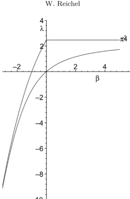
The simplest possible problem is the Fourier-problem
u00+ λu = f on (0, 1), u0(0) = 0, u0(1) + βu(1) = 0.
We are interested in the question how the optimal parameter range for (UAMP) changes with β . The first eigenvalue λ0β1 is given implicitly by
β > 0 : λ0β1 = first positive solution of β =√λ tan√λ β < 0 : λ0β1 = first negative solution of β =p|λ| tanhp|λ|.
Similarly, the first eigenvalue λ∞β1 with zero Dirichlet boundary data at x = 0 is given by
β >−1 : λ∞β1 = first positive solution of β =−√λ cot√λ β <−1 : λ∞β1 = first negative solution of β =−p|λ| cothp|λ|, and λ0∞1 = π2/4 is the first eigenvalue with zero Neumann at x = 0 and zero
Dirichlet at x = 1 . Hence, by Theorem 1 the (UAMP) holds for λ0β1 < λ ≤
2 π /4 λ β –10 –8 –6 –4 –2 2 4 –2 2 4
Figure 5. (UAMP) holds between the two curves
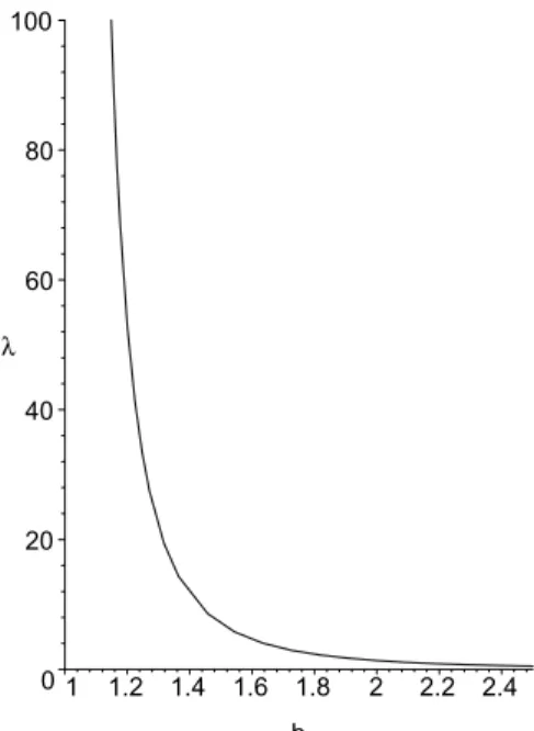
4.2. The radially symmetric Laplacian on annuli
Let Ab ={x ∈ R3 : 1 <|x| < b} be a 3-dimensional annulus. We consider the
boundary value problem
∆u + λu = f in A, ∂νu = 0 on ∂A
under the assumption of radial symmetry f = f (r), u = u(r) . Thus, we have
u00+2
ru
0+ λu = f in (1, b), u0(1) = u0(b) = 0.
Clearly λ001 = 0 (two zero-Neumann boundary conditions). The other two eigen-values λ∞01 (Dirichlet at 1 , Neumann at b ) and λ0∞1 (Neumann at 1 , Dirichlet at b ) can be determined with help of the transformation w(x) = ((b− 1)x + 1)u(b(x− 1) + 1) . The eigenvalue problem then becomes
w00+ λ(b− 1)2w = 0 in (0, 1), λ∞01 : w(0) = 0, w0(1)−b−1b w(1) = 0, λ0∞1 : w0(0)− (b − 1)w(0) = 0, w(1) = 0. Implicitly, the eigenvalues are given by
λ∞01 = µ
(b− 1)2 : µ = first positive solution of
b b− 1 = tan√µ √ µ λ0∞1 = µ
(b− 1)2 : µ = first positive solution of − 1
b− 1 =
tan√µ √
It turns out that λ∞01 < λ0∞1 . Hence, (UAMP) holds for 0 < λ≤ λ∞01 , as shown in Figure 6. 0 20 40 60 80 100 λ 1 1.2 1.4 1.6 1.8 2 2.2 2.4 b
Figure 6. (UAMP) holds between λ001 = 0 and the curve
4.3. The radially symmetric p -Laplacian on balls
On the ball B1(0) ={x ∈ Rn:|x| < 1} in Rn we consider the radially symmetric
boundary value problem
∆pu + λ|u|p−2u = f in B1(0), ∂νu = 0 on ∂B1(0),
i.e., we have
rn−1(|u0|p−2u0)0+ λrn−1|u|p−2u = rn−1f in (0, 1), u0(0) = u0(1) = 0. In this case λN N
1 = 0 . With the help of a Fortran-code described in Brown,
Reichel [2] we computed the eigenvalues λDN
1 and λN D1 . The results for n = 2
and n = 3 are shown in Table 1. It appears that λDN
1 is smaller than λN D1 .
Hence (UAMP) holds between 0 and λDN
p λDN 1 λND1 2.1 0.16953 6.15389 2.5 0.51507 7.71025 3 0.81843 9.83149 4 1.29817 14.68165 5 1.72125 20.34705 6 2.12243 26.82324 7 2.51267 34.10377 8 2.89664 42.18266 9 3.27666 51.05474 10 3.65402 60.71532 p λDN 1 λND1 3.1 0.01023 20.32758 3.5 0.06534 25.21349 4 0.15534 32.21492 5 0.33096 49.43648 6 0.49451 71.35609 7 0.64996 98.45043 8 0.80025 131.18846 9 0.94709 170.03313 10 1.09155 215.44222 Table 1. n = 2 (left) n = 3 (right)
References
[1] M. Arias, J. Campos and J.-P. Gossez, On the antimaximum principle and the Fuˇcik spec-trum of the Neumann p -Laplacian. Differential Integral Equations 13 (2000), 217–226. [2] B.M. Brown and W. Reichel, Computing eigenvalues and Fuˇcik-spectrum of the radially
symmetric p -Laplacian. J. Comput. Appl. Math. 148 (2002), 183-211.
[3] E. A. Coddington and N. Levinson, Theory of Ordinary Differential Equations, McGraw-Hill, New York-Toronto-London, 1955.
[4] Ph. Cl´ement and L.A. Peletier, An anti-maximum principle for second-order elliptic opera-tors. J. Differential Equations 34 (1979), 218–229.
[5] Ph. Cl´ement and G. Sweers, Uniform anti-maximum principle for polyharmonic boundary value problems. Proc. Amer. Math. Soc. 129 (2001), 467–474.
[6] J. Fleckinger, J.-P. Gossez, P. Takaˇc and F. de Th´elin, Existence, nonexistence et principe de l’antimaximum pour le p -laplacien. C. R. Acad. Sci. Paris, t. 321, Serie I (1995), 731–734. [7] J. Fleckinger-Pell´e and P. Takaˇc, Maximum and anti-maximum principles for some elliptic problems. Advances in differential equations and mathematical physics (Atlanta, GA, 1997), 19–32, Contemp. Math. 217, Amer. Math. Soc., Providence, RI, 1998.
[8] T. Godoy, J.-P. Gossez and S. Paczka, Antimaximum principle for elliptic problems with weight. Electronic J. Differential Equations 1999 (1999), No. 22, 1–15.
[9] P. Hess, An anti-maximum principle for linear elliptic equations with an indefinite weight function. J. Differential Equations 41 (1981), 369–374.
[10] P. Lindqvist, Some remarkable sine and cosine functions. Ricerche di Matematica 44 (1995), 269–290.
[11] W. Reichel and W. Walter, Sturm-Liouville type problems for the p -Laplacian under asymp-totic non-resonance conditions. J. Differential Equations 156 (1999), 50–70.
[12] B. Rynne, The Fuˇcik spectrum for general Sturm-Liouville problems. J. Differential Equa-tions 161 (2000), 87–109.
[13] W. Walter, Differential and integral inequalities, Ergebnisse der Mathematik und ihrer Grenzgebiete 55, Springer, Berlin-Heidelberg-New York, 1970.
Wolfgang Reichel Mathematisches Institut Universit¨at Basel Rheinsprung 21 CH-4051 Basel Switzerland
(Received: May 6, 2003)