HAL Id: hal-01365573
https://hal.archives-ouvertes.fr/hal-01365573
Submitted on 13 Sep 2016
HAL is a multi-disciplinary open access
archive for the deposit and dissemination of
sci-entific research documents, whether they are
pub-lished or not. The documents may come from
teaching and research institutions in France or
abroad, or from public or private research centers.
L’archive ouverte pluridisciplinaire HAL, est
destinée au dépôt et à la diffusion de documents
scientifiques de niveau recherche, publiés ou non,
émanant des établissements d’enseignement et de
recherche français ou étrangers, des laboratoires
publics ou privés.
MCTS Experiments on the Voronoi Game
Bruno Bouzy, Marc Métivier, Damien Pellier
To cite this version:
Bruno Bouzy, Marc Métivier, Damien Pellier. MCTS Experiments on the Voronoi Game. International
Conference on Advances in Computer Games, Nov 2011, Tilburg, Netherlands.
�10.1007/978-3-642-31866-5_9�. �hal-01365573�
MCTS Experiments on the Voronoi Game
Bruno Bouzy, Marc M´etivier, and Damien Pellier
LIPADE, Universit´e Paris Descartes, FRANCE,
{bruno.bouzy, marc.metivier, damien.pellier}@parisdescartes.fr
Abstract. Monte-Carlo Tree Search (MCTS) is a powerful tool in games with a finite branching factor. This paper describes an artificial player playing the Voronoi game, a game with an infi-nite branching factor. First, this paper shows how to use MCTS on a discretization of the Voronoi game, and the effects of en-hancements such as RAVE and Gaussian processes (GP). A first set of experimental results shows that MCTS with UCB+RAVE or with UCB+GP are first good solutions for playing the Voronoi game without domain-dependent knowledge. Second, this paper shows how to greatly improve the playing level by using geo-metrical knowledge about Voronoi diagrams, the balance of di-agrams being the key concept. The second set of experimental results shows that a player using MCTS and geometrical knowl-edge outperforms the player without knowlknowl-edge.
1
Introduction
UCT [20], Monte-Carlo Tree Search (MCTS) [12, 8] and RAVE [17] are very pow-erful tools in computer games for games with a finite branching factor. Voronoi diagrams are classical tools in image processing [4, 25]. They have been used to define the Voronoi game (VG) [24, 14], a game with an infinite branching fac-tor. The VG is a good test-bed for MCTS and its enhancements. Furthermore, Gaussian processes (GP) are adapted to find the optimum of a target function in domains with an infinite set of states or actions [23, 6]. Combining MCTS techniques with GP, and testing the result on the VG is the first goal of this pa-per. Our first set of results shows that MCTS with RAVE and GP is an effective solution. In a second stage, this paper shows that domain-dependent knowledge concerning Voronoi diagrams cannot be ommitted. Balance of diagrams is a key concept. This paper shows how to design a MCTS VG player that focusses on balance of cells. Knowledge is used a priori to select a subset of interesting moves used in the tree and in the simulations. The second set of results shows that the MCTS player using Voronoi knowledge outperforms MCTS without knowledge. The outline of the paper is the following. Section 2 defines the Voronoi game. Section 3 mentions work about MCTS, UCT, UCB and RAVE. Section 4 explains how to mix GP and UCB within a MCTS program. Section 5 presents the results obtained with MCTS and GP. Before conclusion, section 6 presents the insertion of relevant Voronoi knowledge into the MCTS algorithm to improve its playing level very significantly.
2
Voronoi Game
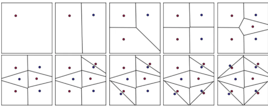
The Voronoi game can be played by several players represented with a color [14]. At his turn, a player puts a site of his color on a 2D square. Each cell around a site gets the color of the site. A colored cell has a area. The area of a player is the sum of the areas of his cells. The game lasts a fixed number of turns (10 in the current work). At the end, the player who gets the largest area wins. In its basic version and in the paper, there are two players, Red and Blue [24], the square is C = [0, 1] × [0, 1], and Red starts. Figure 1 shows the positions of a VG of length 10. Since Blue plays after Red, a komi can be introduced such that Red wins if the area evaluation, Red area minus Blue area, is superior to the komi, the komi value being negative.
Fig. 1: The positions of the Voronoi game of length 10.
Several methods can be used to compute Voronoi diagrams [4, 18, 16, 25, 22]. In order to go forward or backward in a game sequence, the incremental version [4] is appropriate. The computation of areas was helped by [13].
VG can be played on a circle, a segment, a rectangle, or a n-dimensional space as well. VG can be played in the N-round version (the players moves alternately one site per move) or in the one-round version (the players move all their sites in one move) [10]. Key points are essential to play the VG well [1]. Concerning the one-round VG played on a square, [15] proves that the second player always wins. Currently, Jens Anuth master thesis is the most advanced and useful work about VG [2].
3
MCTS, UCT, UCB and RAVE
MCTS (or UCT) repetitively launches simulations starting from the current state. It has four steps: the selection step, the expansion step, the simulation step, and the updating step. In the selection step, MCTS browses a tree from the root down to a leaf by using the UCB rule. To select the next state, UCT chooses the child maximizing the sum of two terms, the mean value and a UCB
term. If x1, . . . , xk are the k children of the current state, then the next state
xnext is selected as follows:
xnext= arg max x∈{x1,...,xk} (µ(x) + ucb(x)) (1) ucb(xi) = s C ×log(T ) Ni (2) µ(xi) is the mean value of returns observed. T is the total number of
sim-ulations in the current state. Ni is the number of simulations in state xi. C is
a constant value set up with experiments. When MCTS reaches a leaf of the tree, it creates one node. Then the simulation uses a random-based policy until the end of the game. At the final state, it gets the return and updates all the mean values of the states encountered in the tree. The UCB rule above balances between exploiting (choose the move with a good mean value to refine existing knowledge) or exploring (choose a move with few trials). The UCB rule works well when the set of moves is finite and pre-defined.
Furthermore, for the game of Go, the RAVE heuristic gave good results [17]. RAVE computes two mean values: the usual one and the AMAF (All Moves As First). The AMAF mean value is updated by considering that all moves of the same color of the first move of the simulation could have been played as the first move. Therefore, after a simulation, it is possible to update the AMAF mean value of all these moves with the return. RAVE uses a weighted mean value of these two mean values. β is the weight driving the balance between the AMAF mean value and the true mean value. K is a parameter set up experi-mentally. When few simulations are performed, β ≈ 0. When many simulations are performed, β ≈ 1, the weight is on the usual mean value.
mRAV E = β × m + (1 − β) × mAM AF (3) β = r Ni K + Ni (4)
4
Light Gaussian Processes
Work concerning bandits on infinite set of actions bound the regret of not playing the best action [19, 3]. The issue is how to generate a finite set of moves that can be provided to UCB to select a move. Gaussian processes (GP) [23, 6] answer the question. At time t, the target function has been observed on points xi with
i = 1, . . . , N . GP aims at finding the next point to try at time t + 1, either a new point or an observed point. The target function is approximated by a surrogate function called f . GP use an acquisition function A to choose the next point at time t + 1. The GP selection needs a matrix inversion which costs a lot of CPU. Since GP selection is called at each node browsed by the tree part of the simulations, it must be fast to execute, and we defined a specific algorithm lighter than GP.
The acquisition function A is defined as a sum of two functions f and g:
∀x ∈ C, A(x) = f (x) + g(x) (5)
For observed points, functions f and g are defined as follows:
∀x ∈ {x1, . . . , xN}, f (x) = µ(x) (6a)
g(x) = ucb(x) (6b)
For never observed points, function f is defined as a weighted mean over the mean values of the observed points:
∀x /∈ {x1, . . . , xN}, f (x) = PN i=1µ(xi) × exp(−a(x − xi)2) PN i=1exp(−a(x − xi) 2) (7)
where a is a constant. Function g is defined as follows: ∀x /∈ {x1, . . . , xN}, g(x) = G ×
N
Y
i=1
(1 − exp(−b(x − xi)2)) (8)
where G and b are constant values.
Finally, the next point to be observed is selected according to the following rule:
xt+1= arg max x∈D
A(x) (9)
where D is a beforehand discretization, or finite subset of C sufficiently large for accuracy, and sufficiently small to evaluate all its elements in practice at every timesteps. When browsing the UCT tree from the root node to a leaf node, the maximization process above is performed in each node. When a leaf node is expanded at the end of browsing, all the children are created following the discretization D. When a node is created, it is virtual, or not observed. It remains virtual until it is tried once, in which case it becomes observed. The size of D is crucial for the speed of the algorithm. When the process terminates, the algorithm returns the move that has the most trials.
The acquisition function A is not continuous: for an observed point xi, A(xi)
is superior to A(x) for x in a small neighbourhood of xi. This allows two kinds
of exploration. When xt+1 is an observed point, the exploration corresponds to
a better estimation of µ(xt+1), or UCB exploration. Otherwise, the exploration
corresponds to the observation of a new point in D. The competition between the two explorations avoids to explore new points before having sufficiently precise estimations of mean values of observed points. The dilemma between the two explorations is managed by G and C.
5
MCTS experiments without knowledge
In this section, the experiments show the relevance of UCB, RAVE and GP to play the Voronoi game without domain-dependent knowledge.
5.1 Calibration experiments
Square C is replaced by a discretization D containing discret × discret points. discret depends on each player. Its value is tuned thanks to calibration tour-naments between several instances of the same player with different values of discret.
Without komi, Blue wins about 85% of games on average, which hinders the search of the best players in a given set. For speeding this search, all games are launched with a komi. The value of the komi depends on the set of players considered. A satisfying value is determined experimentally to make Red and Blue win about 50% of games on average. Experimentally, we used komi ∈ [−0.04, −0.08]. The value is negative reflecting that Blue has the advantage of playing the very important last move.
All experiments are launched with an appropriate simulation number N s. We used N s = 4000. With such value, a player spends between 5 minutes and 10 minutes thinking, and a game lasts between 10 and 20 minutes (a player uses between one and two minutes per move, about 80 random games per second). To compare two players A and B, we launch 50 games with A playing Red and 50 games with A playing Blue. 100 games enables the results to get σ = 5%.
The values of N s and discret interact. For low values of discret, few moves are considered. Although they can be sampled many times, this results in a poor level of play. For large values of discret many moves are considered, but they cannot be sampled sufficiently, resulting in a poor level of play as well. For intermediate values, the resulting program plays at its optimal level. N s being set to 4000, each player has its best value of discret. For UCT, we experimentally found discret = 20.
Tuning C, the UCT constant, is mandatory to make UCT play well. Our experiments showed that C = 0.25 is a good value.
5.2 UCT, RAVE and light GP experiments
Table 1 contains the results of an all-against-all tournament between UCT, RAVE, GP and RGP using N s = 4000. RAVE uses discret = 16 and K = 400. GP uses discret = 26, G = 2 and a = b = 180. RGP uses both enhancement: RAVE+GP. RGP uses discret = 26, G = 2 and a = b = 180. All these values were set beforehand by the calibration experiments.
First, RAVE is superior to UCT (60.5% ± 3%) and GP is superior to UCT (60%±3%). Second, RGP is slightly superior to RAVE (56%±3%) showing that GP is a small enhancement when RAVE is on. RGP is not inferior nor superior to GP (51% ± 3%) showing that RAVE is not an efficient enhancement when GP is on. Third, GP is superior to RAVE (55% ± 3%), which would show that GP is a better enhancement than RAVE. Fourth, the bad news is that RGP is slightly superior only to UCT (54.5% ± 5%), which shows that enhancements are significant by themselves but that their sum is not. Fifth, overall, GP is the best player of our set of experiments regarding the all-against-all tournament total win number. However, time considerations must be underlined: GP and RGP
Table 1: All-against-all results. The cell of row R and column C contains the result of 100 games between R playing Red and C playing Blue: the first number is the number of wins of Red. T indicates the total number of wins. komi = −0.08. N s = 4000.
U CT RAV E GP RGP T U CT 39-61 30-70 43-57 46-54 350 RAV E51-49 56-44 53-47 51-49 399 GP 63-37 63-37 78-22 75-25 428 RGP 55-45 63-37 77-23 80-20 423
spend 13 minutes per game per player while UCT and RAVE spend 5 minutes per game per player. GP (even in its light version) have a heavy computational cost. A fairer assessement between players would give the same thinking time to every players. This would negate the positive effect of GP.
6
MCTS experiments with knowledge
This section shows how to insert Voronoi knowledge into the MCTS framework above, and underlines the improvement in terms of playing level. Jens Anuth thesis describing smart evaluation functions including Voronoi knowledge [2] motivated the work presented in this section. The outline follows the strategical structure of the game:
• the last move special case,
• simple attacks on unbalanced cells and the biggest cell attack, • balance: balanced cells, DB: a defensive balanced player, • BUCT: a UCT player using balanced VD,
• aBUCT: a BUCT player using simple attacks in the simulations, • the one-round game and a second player strategy,
• ABUCT: a BUCT player using sophisticated attacks in the tree.
6.1 The last move special case
The last move is a special case: since the other player will not perform any move after the last move, a depth-one search is the appropriate tool. The result only depends on the discretisation of the square. The higher the discretisation, the better the optimum. The before-last move is also a special case: if the comput-ing power is sufficient, performcomput-ing a depth-two search at the before-last move offers the same upsides than depth-one search at the last move. In the follow-ing subsections, all the players described are assessed by assumfollow-ing that the last and before-last moves are played with depth-one or depth-two minmax strategy respectively.
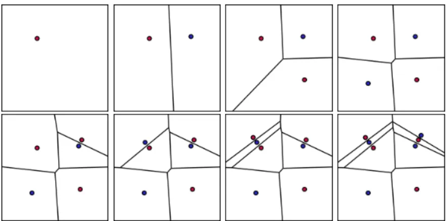
6.2 Simple attacks on unbalanced cells and the biggest cell attack A cell has a gravity center. A straight line intersecting the gravity center of a cell splits this cell into two parts whose size is the half of the given cell. A cell whose site is situated on its gravity center is called a balanced cell, an unbalanced cell otherwise. Figure 2 shows a game that illustrates balanced and unbalanced cells. After moves 1 and 2, the two cells are clearly unbalanced. After move 3, the cells are almost balanced. The most basic attack on an unbalanced cell consists in occupying its gravity center, and consequently in stealing more than the half of the cell. Moves 7 and 8 are simple attacks succeeding on clearly unbalanced cells. Computing the gravity center of a cell is fast and done simultaneously with the area computation. A simple and fast player can be designed by choosing the biggest cell of the opponent and playing on its gravity center. We call this player the biggest-cell-attack player (BCA). The BCA player is very effective against any player creating unbalanced cells without special purpose. Particularly, the BCA player itself produces very unbalanced cells. BCA offers to its opponent the same weakness than the weakness he is exploiting. See moves 5 and 6 of figure 2. Furthermore, the BCA player remains inefficient against players producing balanced cells. Moves 5 and 6 are simple attacks on two cells almost balanced. It is worth noting that BCA wins 60% of games against 400-point-depth-one search. For this reason, in the following, we added the moves generated by the BCA strategy into the set of moves used by depth-one search.
Fig. 2: A Voronoi game with simple cell attacks.
6.3 Balance
Since the BCA player is dangerous for unbalanced cells, playing cells as balanced as possible becomes crucial.
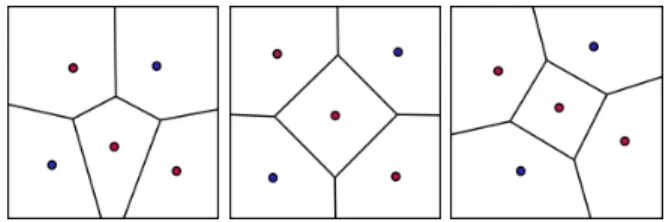
Balanced cells In the VG played on a circle, Ahn defines the importance of key points [1]. The location of a key point does not depend on the player. In a 2 × N round VG, there are N key points that are equally distributed in the circle. Play-ing on them is advised by the best strategy [1]. On the square [10, 15, 2] or any polygon [2], key points are strategically important too. Determining the N key points can be performed with the Lloyd algorithm [21]. The Lloyd algorithm is iterative. It starts with N sites randomly chosen in the square. At each iteration, it moves every sites to the gravity centers of the cells, and computes the resulting VD. In our work, the algorithm stops when the biggest distance between a site and a gravity center reaches a threshold. Since the number of iterations is finite, the VD output of the Lloyd algorithm is not exactly balanced. Figure 3 shows three examples of one color balanced diagrams for the square.
Fig. 3: Three one color balanced diagrams with 5 sites for ten-site Voronoi Game.
DB: a defensive balanced player A very simple defensive program can be designed: the defensive and balanced player (DB). Beforehand, DB computes a balanced one-color VD, and follows it blindly by picking one site at each turn. DB including the last move special case is very good player. If the balanced diagrams are computed offline, DB plays every moves instantly. The result is impressive: DB vs U CT (ns = 1000): 95% and DB vs U CT (ns = 4000): 70%. 6.4 BUCT: a UCT player following balanced VD in the simulations Since balance is important, we aim at integrating it into a UCT player that follows balanced VD in the simulations. Let us call BUCT such a player. Guessing the best balanced one-color VD compatible with the past moves Past moves of the actual game cannot be moved and they have no reason to give balanced one color diagrams. Therefore, for each color, BUCT simulations must follows almost balanced one-color VD compatible with the past moves. The Lloyd algorithm must work with some unmovable sites. This raises two problems. First, the output diagram of the Lloyd algorithm is not necessarily balanced anymore. Second, some random initializations of the opponent sites lead the Lloyd algorithm to local optima. Therefore, the Lloyd algorithm must
be launched several times to avoid local optima, and, for each color, the best balanced diagram is kept.
Using the best balanced one-color VD During the simulations the opponent moves are slight variations around the opponent balanced one color VD, and the friendly moves are slight variations around the friendly balanced one color VD. BUCT is improved with the last move special case as well. The results are very encouraging against UCT: with 1000 simulations BUCT wins 98% of games, 90% (2000 simulations) and 85% (4000 simulations). However, BUCT with 1000, 2000 or 4000 simulations only wins 25% against DB. At this point, the ranking is: U CT ≪ BU CT ≪ DB. UCT has been enhanced into BUCT, but BUCT remains inferior to DB.
6.5 aBUCT: a BUCT player using simple attacks in the simulations Since the BCA strategy is efficient and fast to compute, we have added the BCA strategy in the simulations, which gives a player named aBUCT. In the simulations, the BCA strategy is drawn with probability A1−L where L is the
number of remaining moves in the simulation. The lower the move number in the simulation, the lower the probability to play a BCA move. If the BCA strategy is not drawn then the moves are generated according the simulation policy of BUCT. aBUCT performs very well: with 500 simulations only, it wins 55% of games against DB, and becomes the best player at this point. This result was obtained with A = 2. Other A values in [1, 4] were tested but gave worse results. We observe that adding simple attacks in the simulations improve BUCT from 20% up to 55% against DB, which means BCA is a very efficient enhancement. However, we saw that BCA has difficulties against balanced diagrams. Therefore more sophisticated attacks should give better results. At this point we have: U CT ≪ DB ≤ aBU CT
6.6 The one-round game and the second player strategy 1R2P Since the one-color diagram balance is important, let us consider the one-round game [10]. The one round VG differs with the N-round VG in that Red plays all his sites first (in one round), and Blue plays all his sites second. We are interested in finding out second player strategies defeating arbitrary red VD. Assume a red diagram is given with N cells. Blue, the second player, has N moves to play in a row to win the game. This is a planning problem. To solve it, the simplest tool consists in playing the BCA strategy N times. This tool works well for any unbalanced red diagram. Then, a smarter tool is to use the idea of Fekete [15]. It consists in playing the first move with a depth-one search, and the following moves with the BCA strategy. It works on the square example and N = 4 in [15]. One may extend the Fekete’s idea by using the one-round second player (1R2P) strategy.
B=0 repeat
play the depth-one strategy B times play the BCA strategy N-B times B=B+1
until success or B>N
The 1R2P strategy iteratively tries combinations of playing depth-one strate-gies B times and BCA stratestrate-gies N − B times. While failures are encountered, 1R2P tries to solve the problem again by incrementing B. Theoretically, since complex combinations of blue sites might be necessary to beat complex red bal-anced diagrams, the algorithm 1R2P is not proven to be complete. However, in practice, along all our experiments, 1R2P always returned a successful strategy. With N = 5, 1R2P never needed B being greater than 2. Let Aggressive(V ) be the blue diagram obtained by 1R2P in the one-round VG starting with the red diagram V .
6.7 ABUCT: a BUCT player using sophisticated attacks in the tree With the possibility to build aggressive diagrams defeating balanced diagrams, we are now able to set up a new player called Agressive and Balanced UCT (ABUCT). Beforehand, ABUCT computes the red and blue balanced diagrams adequate to the past moves actually played: RedBD and BlueBD. Then, ABUCT computes Aggressive(RedBD) and Aggressive(BlueBD) with the 1R2P strat-egy on the one-round game. Then, ABUCT launches the UCT simulations with moves generated according to the balanced diagrams and to the agres-sive diagrams in the tree part of UCT. The results are excellent. With 500 simulations only, ABUCT wins 71% against aBUCT, 93% against UCT (500 simulations as well), and importantly 77% against DB. To sum up, we have: U CT ≪ DB ≤ aBU CT ≪ ABU CT .
6.8 Against human players and against other work
As seen above, playing diagrams as balanced as possible is crucial. Human players (H) can be good to roughly see the balance of a diagram. However, they cannot be as precise as the Lloyd algorithm. Furthermore, the precision of a mouse click on a GUI point is is a burden for human players. This lack of precision limits the human level below the level of simple artificial players such as BCA. Despite of this, human players may defeat UCT of section 3. Existing other work consist in some applets [24, 14] using simple players such as BCA, and the work of Jens Anuth [2]. Although the Anuth’s program can play on arbitrary polygons, the best player of Anuth’s work corresponds to DB. We observed that: U CT ≤ H ≤ BCA ≪ DB ≪ ABU CT .
7
Conclusion
We have shown a successful adaptation of MCTS in a game with an infinite branching factor, the Voronoi game. We tested UCT with RAVE and GP. They gave results strictly better than UCT alone (60% of wins). Adding Voronoi knowledge is essential to improve the playing level. A simple knowledge-based player such as DB outperforms UCT with 4000 simulations (70%). We have shown how to insert fundamental concepts such as biggest cell attack, bal-anced one-color diagram, one-round game heuristic, into UCT, yielding suc-cessive versions of UCT: BUCT, aBUCT and ABUCT, an aggressive and bal-anced UCT player using 500 simulations that obtains 93% of wins against UCT using the same number of simulations. As in Go [5], inserting domain-dependent knowledge into the simulations improves the playing level. Our study shows that domain dependent knowledge brings about improvements far better than the improvements brought about by RAVE or GP. To sum up, we have: U CT ≤ RAV E ≈ GP ≪ DB ≤ aBU CT ≪ ABU CT .
Future works are numerous. First, make the length of a VG vary would bring information about the robustness of our approaches. Second, make the ABUCT player use several friendly balanced diagrams per color instead of one, and sev-eral aggressive balanced diagrams per color, and make the options at some nodes of the tree be the strategies following these diagrams. Third, smooth the transi-tion between the strategy used in the middle game (UCT with knowledge) and the strategy used in the last moves (minmax search). An intermediate strategy keeping the best of both strategies remains to be found. Fourth, compare other approaches optimizing a function in a continuous space such as HOO [7], or progressive widening [9, 11] with our light GP approach (section 4). Fifth, define a multi-player VG and test the ability of MCTS on multi-player games with an infinite branching factor. Finally, popularizing the VG to give birth to other artificial VG players is an enjoying perspective.
8
Acknowledgements
This work has been supported by French National Research Agency (ANR) through COSINUS program (project EXPLO-RA number ANR-08-COSI-004).
References
1. Hee-Kap Ahn, Siu-Wing Cheng, Otfried Cheong, Mordecai Golin, and Ren´e van Oostrum. Competitive facility location: the Voronoi game. Theoretical Computer Science, 310(1-3):457–467, 2004.
2. Jens Anuth. Strategien fur das Voronoi-spiel. Master’s thesis, FernUniveristat in Hagen, July 2007.
3. Peter Auer, Ronald Ortner, and Csaba Szepesvari. Improved rates for the stochas-tic continuum-armed bandit problem. In N. Bshouty and C. Gentile, editors, COLT, volume 4539 of LNAI, pages 454–467. Springer-Verlag, 2007.
4. Franz Aurenhammer. Voronoi diagrams: a survey of a fundamental geometric data structure. ACM Computing Surveys, 23(3):345–405, 1991.
5. Bruno Bouzy. Associating domain-dependent knowledge and Monte-Carlo ap-proaches within a go playing program. Information Sciences, 175(4):247–257, 2005. 6. Eric Brochu, Vlad Cora, and Nando de Freitas. A tutorial on bayesian optimization of expensive cost functions, with application to active user modeling and hierar-chical reinforcement learning. Technical Report 23, Univ. of Brit. Col., 2009. 7. S´ebastien Bubeck, R´emi Munos, Gilles Stoltz, and Csaba Szepesv´ari. X-armed
bandits. Journal of Machine Learning Research, 12:1655–1695, 2011.
8. Guillaume Chaslot. Monte-Carlo Tree Search. PhD thesis, Maastricht Univ., 2010. 9. Guillaume Chaslot, Mark Winands, Jaap van den Herik, Jos Uiterwijk, and Bruno Bouzy. Progressive strategies for Monte-Carlo tree search. New Mathematics and Natural Computation, 4(3):343–357, 2008.
10. Otfried Cheong, Sariel Har-Peled, Nathan Linial, and Jiˇr´ı Matouˇsek. The one-round Voronoi game. In 18th Symposium on Computational Geometry, pages 97– 101. ACM, 2002.
11. Adrien Cou¨etoux, Jean-Baptiste Hoock, Nataliya Sokolovska, Olivier Teytaud, and Nicolas Bonnard. Continuous upper confidence trees. In Proceedings of the 5th International Conference on Learning and Intelligent OptimizatioN (LION), 2011. 12. R´emi Coulom. Efficient selectivity and backup operators in Monte-Carlo tree search. In J.H. van den Herik, P. Ciancarini, and H.H.L.M. Donkers, editors, Computers and Games, volume 4630 of LNCS, pages 72–83. Springer-Verlag, 2006. 13. Frank Dehne, Rolf Klein, and Raimund Seidel. Maximizing a Voronoi region: The convex case. In Algorithms and Computation, 13th International Symposium, ISAAC, volume 2518 of LNCS, pages 185–193. Springer-Verlag, 2002.
14. Monty Faidley, Chris Poultney, and Dennis Shasha. The Voronoi game. http://home.dti.net/crispy/Voronoi.html.
15. S´andor P. Fekete and Henk Meijer. The one-round Voronoi game replayed. Com-putational Geometry Theory Appl., 30:81–94, 2005.
16. Steven Fortune. A sweepline algorithm for Voronoi diagrams. Algorithmica, 2(2):153–174, 1987.
17. Sylvain Gelly and David Silver. Achieving master level play in 9x9 computer go. In AAAI, pages 1537–1540, 2008.
18. Leo J. Guibas and Jorge Stolfi. Primitives for the manipulation of general subdi-visions and the computation of Voronoi diagrams. In 15th ACM Symposium on Theory Of Computing, pages 221–234. ACM, 1983.
19. Robert Kleinberg. Nearly tight bounds for the continuum-armed bandit problem. In NIPS 17, pages 697–704. MIT Press, 2005.
20. Levente Kocsis and Csaba Szepesvari. Bandit based Monte-Carlo planning. In European Conference on Machine Learning, volume 4212 of LNCS/LNAI, pages 282–293, 2006.
21. Stuart P. Lloyd. Least squares quantization in PCM. IEEE Transactions on Information Theory, 28:129–137, 1982.
22. Mir Abolfazl Mostafavi, Christopher Gold, and Maciej Dakowicz. Delete and in-sert operations in Voronoi/Delaunay methods and applications. Computers and Geosciences, 29(4):523–530, 2003.
23. Carl Edward Rasmussen and Christopher K. I. Williams. Gaussian Processes for Machine Learning. MIT Press, 2006.
24. Indrit Selimi. The Voronoi game, 2008. http://www.voronoigame.com/.
25. Jonathan Shewchuk. Triangle: Engineering a 2d quality mesh generator and Delaunay triangulator. In Work. on Appl. Comp. Geom., pages 203–222, 1996.