HAL Id: hal-01393927
https://hal.inria.fr/hal-01393927
Submitted on 8 Nov 2016
HAL is a multi-disciplinary open access
archive for the deposit and dissemination of sci-entific research documents, whether they are pub-lished or not. The documents may come from teaching and research institutions in France or abroad, or from public or private research centers.
L’archive ouverte pluridisciplinaire HAL, est destinée au dépôt et à la diffusion de documents scientifiques de niveau recherche, publiés ou non, émanant des établissements d’enseignement et de recherche français ou étrangers, des laboratoires publics ou privés.
Maximal cliques structure for cocomparability graphs
and applications
Jérémie Dusart, Michel Habib, Derek G. Corneil
To cite this version:
Jérémie Dusart, Michel Habib, Derek G. Corneil. Maximal cliques structure for cocomparability graphs and applications. 2016. �hal-01393927�
Maximal cliques structure for cocomparability graphs
and applications
J´er´emie Dusart
∗, Michel Habib
∗†and Derek G. Corneil
‡November 7, 2016
Abstract
A cocomparability graph is a graph whose complement admits a transitive orien-tation. An interval graph is the intersection graph of a family of intervals on the real line. In this paper we investigate the relationships between interval and cocomparabil-ity graphs. This study is motivated by recent results [5, 13] that show that for some problems, the algorithm used on interval graphs can also be used with small modifica-tions on cocomparability graphs. Many of these algorithms are based on graph searches that preserve cocomparability orderings.
First we propose a characterization of cocomparability graphs via a lattice structure on the set of their maximal cliques. Using this characterization we can prove that every maximal interval subgraph of a cocomparability graph G is also a maximal chordal subgraph of G. Although the size of this lattice of maximal cliques can be exponential in the size of the graph, it can be used as a framework to design and prove algorithms on cocomparability graphs. In particular we show that a new graph search, namely Local Maximal Neighborhood Search (LocalMNS) leads to an O(n + mlogn) time algorithm to find a maximal interval subgraph of a cocomparability graph. Similarly we propose a linear time algorithm to compute all simplicial vertices in a cocomparability graph. In both cases we improve on the current state of knowledge.
Keywords: (co)-comparability graphs, interval graphs, posets, maximal antichain
lat-tices, maximal clique latlat-tices, graph searches.
1
Introduction
This paper is devoted to the study of cocomparability graphs, which are the complements of comparability graphs. A comparability graph is simply an undirected graph that admits a
∗IRIF, CNRS & Universit´e Paris Diderot, Paris, France †Gang, Inria Paris
transitive acyclic orientation of its edges. Comparability graphs are well-studied and arise naturally in the process of modeling real-life problems, especially those involving partial orders. For a survey see [17, 33]. We also consider interval graphs which are the intersection graphs of a family of intervals on the real line. Comparability graphs and cocomparability graphs are well-known subclasses of perfect graphs [17]; and interval graphs are a well-known subclass of cocomparability graphs [3]. Clearly a given cocomparability graph G together with an acyclic transitive orientation of the edges of G (the corresponding comparability
graph) can be equivalently represented by a poset PG; thus new results in any of these three
areas immediately translate to the other two areas. In this paper, we will often omit the translations but it is important to keep in mind that they exist.
A triple a, b, c of vertices forms an asteroidal triple if the vertices are pairwise independent, and every pair remains connected when the third vertex and its neighborhood are removed from the graph. An asteroidal triple free graph (AT-free for short) is a graph with no asteroidal triples. It is well-known that AT-free graphs strictly contain cocomparability graphs, see [17].
A classical way to characterize a cocomparability graph is by means of an umbrella-free total ordering of its vertices. In an ordering σ of G’s vertices, an umbrella is a triple of
vertices x, y, z such that x <σ y <σ z, xy, yz /∈ E(G), and xz ∈ E(G). It has been
observed in [26] that a graph is a cocomparability graph if and only if it admits an umbrella-free ordering. We will also call an umbrella-umbrella-free ordering a cocomp ordering. In a similar way, interval graphs are characterized by interval orderings, where an interval ordering σ is an ordering of the graph’s vertices that does not admit a triple of vertices x, y, z such that
x <σ y <σ z, xy /∈ E(G), and xz ∈ E(G). (Notice that an interval ordering is a cocomp
ordering.) Other characterizations of interval graphs appear in theorem 2.14.
The paper studies the relationships shared by interval and cocomparability graphs and is motivated by some recents results:
• For the Minimum Path Cover (MPC) Problem (a minimum set of paths such that each vertex of G belongs to exactly one path in the set), Corneil, Dalton and Habib showed that the greedy MPC algorithm for interval graphs, when applied to a Lexico-graphic Depth First Search (LDFS) cocomp ordering provides a certifying solution for cocomparability graphs (see [5]).
• For the problem of producing a cocomp ordering (assuming the graph is cocompa-rability) Dusart and Habib showed that the multisweep Lexicographic Breadth First
Search (LBFS)+ algorithm to find an interval ordering also finds a cocomp ordering
([13]). Note that O(|V (G)|) LBFSs must be used in order to guarantee these results.
Other similar results will be surveyed in subsection 3.2. From these results, some natural questions arise: Do cocomparability graphs have some kind of hidden interval structure that allows the “lifting” of some interval graph algorithms to cocomparability graphs? What is the role played by graph searches LBFS and LDFS and are there other searches/problems where similar results hold?
As mentioned previously, interval graphs form a strict subclass of cocomparability graphs. It is also known that every minimal triangulation of a cocomparability graph is an interval graph [34, 31]. In section 2 of this article, we will show that we can equip the set of maximal cliques of a cocomparability graph with a lattice structure where every chain of the lattice forms an interval graph. Note that condition (iii) of theorem 2.14 states that a graph G is an interval graph if and only if the maximal cliques of G can be linearly ordered so that for every vertex x, the cliques containing x appear consecutively. Thus, through the lattice, a cocomparability graph can be seen as a special composition of interval graphs. In particular,
given a cocomparability graph G with P a transitive orientation of G, the lattice MA(P )
is formed on the set of maximal antichains of P (i.e., the maximal cliques of G). A graph
H = (V (H), E(H)) with E(H)⊆ E(G) is a maximal chordal (respectively interval) subgraph
if and only if H is a chordal graph and∀S ⊆ E(G)−E(H), S 6= ∅, H0 = (V (H), E(H)∪S) is
not a chordal (respectively interval) graph. Our final result of subsection 2.4 states that every maximal interval subgraph of a cocomparability graph is also a maximal chordal subgraph. In sections 3 and 4 we turn our attention to algorithmic applications of the theory
pre-viously developed on the lattice MA(P ). In section 3 we present algorithm Chainclique
which on input a graph G and a total ordering σ of V (G) returns an ordered set of cliques that collectively form an interval subgraph of G. We then introduce a new graph search (LocalMNS) that is very close to Maximal Neighborhood Search (MNS), which is a gener-alization of MCS, LDFS and LBFS. We show that Chainclique with σ being a LocalMNS cocomparability ordering of G returns a maximal interval subgraph of the cocomparability graph G; this algorithm also gives us a way to compute a minimal interval extension of a partial order (definitions given in subsection 1.1). Section 4 uses Chainclique to compute the set of simplicial vertices in a cocomparability graph.
Concluding remarks appear in section 5.
1.1
Notation
In this article, for graphs we follow standard notation; see, for instance, [17]. All the graphs considered here are finite, undirected, simple and with no loops. An edge between vertices u and v is denoted by uv, and in this case vertices u and v are said to be adjacent. G denotes
the complement of G = (V (G), E(G)), i.e., G = (V (G), E(G)), where uv ∈ E(G) if and only
if u 6= v and uv /∈ E(G). Let S ⊆ V (G) be a set of vertices of G. Then, the subgraph of G
induced by S is denoted by G[S], i.e., G[S] = (S, F ), where for any two vertices u, v ∈ S,
uv ∈ F if and only if uv ∈ E(G). The set N(v) = {u ∈ V (G)|uv ∈ E(G)} is called the
neighborhood of the vertex v ∈ V (G) in G = (V (G), E(G)). A vertex v is simplicial if
G[N (v)∪ {v}] is a clique. An ordering σ of V (G) is a permutation of V (G) where σ(i) is
the i’th vertex in σ; σ−1(x) denotes the position of x in σ. For two vertices u, v, we write
that u <σ v if and only if σ−1(u) < σ−1(v). For two vertices u, v ∈ V (G), we say that u is
left (respectively right) of v in τ if u <τ v (respectively v <τ u).
For partial orders we use the following notation. A partial order (also known as a poset)
P = (X,≤P) is an ordered pair with a finite set X, the ground set of P , and with a binary
x≤P y or y ≤P x then x, y are comparable, otherwise they are incomparable and denoted by
xkP y. We will also use the covering relation in P denoted by ≺P, satisfying x≺P y if and
only if x ≤P y and ∀z such that x ≤P z ≤P y then x = z or z = y. In such a case we say
that “y covers x” or that “x is covered by y”.
A chain (respectively an antichain) is a partial order in which every pair (respectively no pair) is comparable. As mentioned previously, a given cocomparability graph G and a
transitive orientation of the edges of G can be equivalently represented by a poset PG. Note
that a chain (respectively an antichain) in PGcorresponds to an independent set (respectively
a clique) in G. An extension of a partial order P = (X,≤P) is a partial order P0 = (X,≤P0),
where for u, v ∈ X, u ≤P v implies u ≤P0 v. In particular, if P0 is a chain then P0 is called
a linear extension of P . An interval extension of a partial order is an extension that is also an interval order (interval orders are acyclic transitive orientations of the complement of
interval graphs). P− is the poset obtained from P by reversing all comparabilities.
A lattice is a particular partial order L = (L,≤L)1 for which each two-element subset
{a, b} ⊆ L has a join (i.e., least upper bound) and a meet (i.e., greatest lower bound),
denoted by a∨ b and a ∧ b respectively. This definition makes ∧ and ∨ binary operations
on L. All the lattices considered here are assumed to be finite. A distributive lattice is one in which the operations of join and meet distribute over each other; a modular lattice is a
lattice that satisfies the following self-dual condition: x≤ b implies x ∨ (a ∧ b) = (x ∨ a) ∧ b
for all a. For other definitions on lattices, the reader is referred to [2, 18, 10, 37, 4].
2
Lattice characterization of cocomparability graphs
2.1
The maximal antichain lattice of a partial order
It is known from Birkhoff [2]2 thatA(P ), the set of all antichains of a partial order P , can be
equipped with a lattice structure using the following relation between antichains: if A, B are
two antichains in P then A≤A(P ) B if and only if∀a ∈ A, ∃b ∈ B with a ≤P b. Furthermore,
it is also well-known that the lattice A(P ) = (A(P ), ≤A(P )) is a distributive lattice.
We now consider the relation ≤MA(P ), which is the restriction of the relation ≤A(P ) to
the set of all maximal (with respect to set inclusion) antichains of P denoted by MA(P ).
Let us now review the main results known aboutMA(P ) = (MA(P ), ≤MA(P )).
The next lemma shows that the definition of ≤MA(P ) can be written symmetrically in
the 2 antichains A and B, since they are maximal antichains.
Lemma 2.1. [1] Let A, B be two maximal antichains of a partial order P .
A ≤MA(P ) B if and only if ∀a ∈ A, ∃b ∈ B with a ≤P b if and only if ∀b ∈ B, ∃a ∈ A
with a≤P b.
1Note that we use the same symbol, namely L for both the lattice and the ground set of the lattice; the
exact meaning will be clear from the context.
2Indeed Birkhoff studied the ideal lattice of a partial order, but there exists a natural bijection between
Some helpful variations:
Lemma 2.2. Let A, B be two maximal antichains of a partial order P .
A <MA(P ) B if and only if ∀a ∈ A, ∃b ∈ B with a <P b if and only if ∀b ∈ B, ∃a ∈ A
with a <P b.
Lemma 2.3. LetA, B be two maximal antichains of a partial order P such that A ≤MA(P )B.
If x∈ A, y ∈ B then x ≤P y or xkP y.
Proof. We have two cases: either A = B or A6= B. In the first case, since A is an antichain
and A = B, we get ∀x ∈ A, ∀y ∈ A, if x 6= y then x kP y and if x = y then x≤P y.
In the second case, suppose for contradiction there exists x∈ A, y ∈ B such that y <P x.
Since we are in the case where A and B are different maximal antichains, and since x and
y are comparable, necessarily we have x ∈ A-B, y ∈ B-A and also A ≤MA(P ) B. Applying
lemma 2.1 on A and B, there exists z ∈ A-B such that z ≤P y. By transitivity of P , we
establish that z≤P x, therefore contradicting A being an antichain.
Now we focus on an interesting consecutiveness property in MA(P ).
Proposition 2.4. Let A, B, C be three maximal antichains of a partial order P such that
A≤MA(P ) B ≤MA(P ) C; then A∩ C ⊆ B.
Proof. In the case where A = B we have that A ∩ C ⊆ B and in the case B = C we
have that A∩ C ⊆ B. So we can assume that A 6= B, B 6= C and as a consequence that
A <MA(P ) B <MA(P )C. Suppose for sake of contradiction that A∩ C 6⊆ B. So there exists
x∈ (A ∩ C)-B. Since x does not belong to B there must exist some y ∈ B comparable to x.
Using lemma 2.3 on A, B we establish that x≤P y. Again using lemma 2.3 on B, C we get
that y ≤P x. Since x≤P y and y ≤P x, necessarily y = x. Therefore x belongs to B which
contradicts x∈ (A ∩ C)-B.
The covering relation between maximal antichains has also been characterized.
Lemma 2.5. [24] Let A, B be two different maximal antichains of a partial order P .
A≺MA(P ) B if and only if ∀x ∈ A-B and ∀y ∈ B-A, x ≺P y.
Proof. Suppose that A≺MA(P ) B and let y ∈ B-A. Further suppose that y does not cover
some x∈ A-B. Note that either x ≤P y or y kP x. In the first case, x ≤P y, and thus there
exists z such that x≤P z ≤P y. But then consider A0the set obtained from A by: exchanging
x and z; deleting all vertices comparable with z and adding all successors of x incomparable
with z. A0 is a maximal antichain by construction and we have: A
≤MA(P ) A0 ≤MA(P ) B, a
contradiction.
In the second case, y kP x, where x∈ A-B. Let us consider A0 ={z ∈ A-y | z ≺P y}+y.
We complete A0 as a maximal antichain [A0] by adding elements of A
∪ B. Since x, y ∈ [A0],
[A0] 6= A and [A0] 6= B. Then we have: A <
MA(P ) [A0] <MA(P ) B, a contradiction to
Conversely, clearly we have A ≤MA(P ) B. Let us now prove that B covers A; if not,
there exists some maximal antichain A0 such that A <
MA(P ) A0 <MA(P ) B. Let y ∈ B-A0;
there exists z ∈ A0 with z <
P y. Using Proposition 2.4 we know that A∩ B ⊆ A0; then
necessarily z /∈ A. Thus there exists x ∈ A-B with x <P z, but then y is not covered by x a
contradiction.
We now introduce some new terminology in order to define the infimum and supremum
on the lattice MA(P ).
Definition 2.6. For a partial order P = (X,≤P), S ⊆ X, Max(S) = {v ∈ S | ∀u ∈ S, u ≤P
v or ukP v}. Max(S) is the set of maximal elements of the partial order P (S) induced by
S. In the same way, M in(S) = {v ∈ S | ∀u ∈ S, v ≤P u or u kP v}. Min(S) is the set
of minimal elements of P (S). And Inc(S) = {x ∈ X − S | ∀y ∈ S, x kP y} is the set of
incomparable elements to S.
Definition 2.7. For two antichains A, B of a partial order P = (X,≤P), let Smin(A, B) =
{x ∈ A-B | ∃y ∈ B-A with x <P y} and Smax(A, B) ={x ∈ A-B | ∃y ∈ B-A with y <P x}.
Since A, B are antichains, we necessarily have: Smin(A, B)∩ Smax(A, B) =∅.
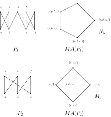
a b c d e f {d, e, f} {a, b, c} {a, f} {b, d} {c, e} a b c d e f g h i {a, b, c, d} {e, f, g, h, i} {c, d, e, f} {a, b, h, i} {a, g, h, i} P1 M A(P1) M A(P2) P2 N5 M3
Figure 1: Two orders whose maximal antichain lattices are respectively N5 and M3, the smallest
non distributive lattices.
As an example of these definitions consider the partial order P1 of Figure 1. If we take
Smin(A, B) = {a}, Smax(A, B) = {g, h, i}, Smin(B, A) = {c, d}, Smax(B, A) = {e, f}. From
these definitions we see:
Proposition 2.8. Let A, B be two maximal antichains of a partial order P , then (A∩
B), Smin(A, B) and Smax(A, B) partition A.
Proof. Let us consider a vertex x of A. We have two cases: either x∈ B or x /∈ B. In the first
case x ∈ A ∩ B. In the second case, since B is a maximal antichain and x /∈ B, there must
exist y ∈ B such that y is comparable to x. Since y ∈ B and x /∈ B, we deduce that y 6= x.
Therefore we have two cases: either x <P y or y <P x. In the first case, x∈ Smin(A, B) and
in the second case x ∈ Smax(A, B). Thus A = (A∩ B) ∪ Smin(A, B)∪ Smax(A, B) and by
definition these 3 sets do not intersect.
It should be noticed that in the well-known distributive lattice of antichains A(P ), the
infimum A∧A(P )B = (A∩ B) ∪ Smin(A, B)∪ Smin(B, A) and the supremum A∨A(P )B =
(A∩ B) ∪ Smax(A, B)∪ Smax(B, A).
In this definition A∧A(P )B and A∨A(P )B are clearly antichains, but they are not maximal
even if A, B are maximal. For example in P1in Figure 1 we have{a, g, h, i}∨A(P ){c, d, e, f} =
{e, f, h, i} which is not maximal.
Therefore we can now define the infimum and supremum and MA(P ) as follows:
Definition 2.9. For two maximal antichains A, B of a partial order P , we define the binary
operators ∧MA(P ),∨MA(P ):
infimum: A ∧MA(P ) B = (A ∩ B) ∪ Smin(A, B) ∪ Smin(B, A) ∪ Max(Inc((A ∩ B) ∪
Smin(A, B)∪ Smin(B, A))) = A∧A(P )B ∪ Max(Inc(A ∧A(P )B)).
supremum: A ∨MA(P ) B = (A∩ B) ∪ Smax(A, B)∪ Smax(B, A)∪ Min(Inc((A ∩ B) ∪
Smax(A, B)∪ Smax(B, A))) = A∨A(P )B∪ Max(Inc(A ∨A(P )B)).
Returning to the partial order P1 of Figure 1 where A ={a, g, h, i} and B = {c, d, e, f} we
see that M ax(Inc((A∩ B) ∪ Smin(A, B)∪ Smin(B, A))) = {b}. Therefore {a, g, h, i} ∧MA(P )
{c, d, e, f} = {a, b, c, d}. Similarly {a, g, h, i} ∨MA(P ){c, d, e, f} = {e, f, g, h, i}, whereas in
A(P ) we have: {a, g, h, i} ∨A(P ){c, d, e, f} = {e, f, h, i} ( {a, g, h, i} ∨MA(P ){c, d, e, f}.
Since the above supremum and infimum definitions are differently expressed compared to those of [1], for completeness we give a proof of the following theorem due to Berhendt.
Theorem 2.10. [1] Let P be a partial order. MA(P ) = (MA(P ), ∧MA(P ),∨MA(P )) is a
lattice.
Proof. Let us first consider A∧MA(P )B. Clearly elements of Smin(A, B) are incomparable
with elements of Smin(B, A). Therefore (A∩ B) ∪ Smin(A, B)∪ Smin(B, A) is an antichain of
P . Adding to it M ax(Inc((A∩ B) ∪ Smin(A, B)∪ Smin(B, A))) completes it as a maximal
antichain.
Since A, B are maximal antichains, for every x∈ Inc((A ∩ B) ∪ Smin(A, B)∪ Smin(B, A))
there exists t ∈ Smax(A, B) and z ∈ Smax(B, A) both comparable with x. If t ≤P x, since
there exists y ∈ B such that y ≤P t, it would imply by transitivity: y ≤p x which is
Therefore we have:
A∧MA(P )B ≤MA(P ) A and A∧MA(P )B ≤MA(P ) B.
Now let us consider a maximal antichain C, such that: C ≤MA(P ) A and C ≤MA(P )B.
But for every c ∈ C, there exists some a ∈ A with c ≤P a. If a does not belong to
(A∩ B) ∪ Smin(A, B) then a ∈ Smax(A, B) and so there exists z ∈ Max(Inc((A ∩ B) ∪
Smin(A, B)∪ Smin(B, A))), with c≤P a≤P z. Thus C≤MA(P ) A∧MA(P )A. Symmetrically
one can obtain C ≤MA(P )A∧MA(P )B.
Therefore this binary relation ∧MA(P ) defined on maximal antichains behaves as an
infi-mum relation on maximal antichains.
The proof is similar for ∨MA(P ).
Proposition 2.11. Let A, B be two maximal antichains of a partial order P .
Then (A∪ B) ⊆ (A ∨MA(P )B)∪ (A ∧MA(P )B).
Proof. Using the definition of A∧MA(P )B, we get that (A∩ B) ∪ Smin(A, B)∪ Smin(B, A)⊆
(A∧MA(P ) B) and symmetrically with A ∨MA(P ) B we get that (A∩ B) ∪ Smax(A, B)∪
Smax(B, A)⊆ (A ∨MA(P )B).
By proposition 2.8, we know that A = (A∩ B) ∪ Smin(A, B)∪ Smax(A, B) and B =
(A∩B)∪Smin(B, A)∪Smax(B, A), thereby showing (A∪B) ⊆ A∨MA(P )B∪(A∧MA(P )B).
Corollary 2.12. Let A, B be two maximal antichains of a partial order P where x∈ A − B.
Then we have two mutually exclusive cases: either x∈ (A ∧MA(P )B) or x∈ (A ∨MA(P )B).
Proof. Let A, B be two maximal antichains of a partial order P where x ∈ A-B. Then
either x∈ (A∧MA(P )B) or otherwise (using proposition 2.11), necessarily x∈ (A∨MA(P )B).
From proposition 2.8, A-B is partitioned into Smin(A, B) ⊆ A ∧MA(P )B and Smax(A, B)⊆
A∨MA(P )B. Therefore the two cases are mutually exclusive.
There are two natural questions that arise concerning the lattice MA(P ) for a given
partial order P , namely:
• Does MA(P ) have a particular lattice structure?
• What is the maximum size of MA(P ) given n, the number of elements in P ?
The answer to the first question is “no” since Markowsky in [28] and [29] showed that any finite lattice is isomorphic to the maximal antichain lattice of a height one partial order. This result has been rediscovered by Berhendt in [1]. This is summarized in the next theorem.
Theorem 2.13. [1, 28, 29] Any finite lattice is isomorphic to the lattice MA(P ) of some
In particular, as shown in Figure 1 or using the previous theorem, MA(P ) is not always
distributive, thereby showing that MA(P ) is not a sublattice of A(P ) as already noticed in
[1]. Jakub´ık in [24] studied for which partial orders P , MA(P ) is modular.
For the second question, the size ofMA(P ) can be exponential in the number of elements
of P . If we consider a poset P made up of k disjoint chains of length 2, MA(P ) has
exponential size since P has 2k maximal antichains. The example of Figure 2 shows the
k = 2 case. Furthermore Reuter showed in [36] that even the computation of the maximum
length of a directed path (i.e., the height) in MA(P ) is an NP-hard problem when only P
is given as the input.
a b c d e f {a, b} {a, d} {a, f} {b, c} {b, e} {c, d} {d, e} {c, f} {e, f}
Figure 2: MA(P ) for k = 2.
2.2
Maximal antichain lattice and interval orders
Following [17] interval graphs can be defined and characterized: Theorem 2.14. [16, 27]
The following propositions are equivalent and characterize interval graphs.
(i) G can be represented as the intersection graph of a family of intervals of the real line.
(ii) There exists a total ordering τ of the vertices of V such that ∀x, y, z ∈ G with
x≤τ y≤τ z and xz ∈ E then xy ∈ E.
(iii) The maximal cliques of G can be linearly ordered such that for every vertex x of G,
the maximal cliques containing x occur consecutively.
(iv) G contains no chordless 4-cycle and is a cocomparability graph. (v) G is chordal and has no asteroidal triple.
As mentioned in the Introduction, an ordering of the vertices satisfying condition (ii) is called an interval ordering and interval orders are acyclic transitive orientations of the complement of interval graphs. Therefore we have the following characterization theorem: Theorem 2.15. The following propositions are equivalent and characterize interval orders:
(i) P can be represented as a left-ordering of a family of intervals of the real line.
(ii) The successors sets are totally ordered by inclusion. (iii) The predecessors sets are totally ordered by inclusion;
(iv) P has a maximal antichain path. (A maximal clique path is just a maximal clique tree T, reduced to a path).
(v) P does not contain a suborder isomorphic to 2+ 2 (See Figure 3).
a • b • c • d•
Figure 3: A 2 + 2 partial order
In terms of the lattice MA(P ), condition (iv) becomes:
Proposition 2.16. [1] P is an interval order if and only if MA(P ) is a chain.
This result can be complemented by:
Theorem 2.17. [21] The minimal interval order extensions of P are in a one-to-one
cor-respondence with the maximal chains of MA(P ).
As a consequence developed in [21], the number of minimal interval orders extensions of P is a comparability invariant and is #P-complete to compute. For additional background information on interval orders, the reader is encouraged to consult Fishburn’s monograph [15] or Trotter’s survey article [38].
2.3
Maximal cliques structure of cocomparability graphs
In the following, we first characterize cocomparability graphs in terms of a particular lattice structure on its maximal cliques and show that it extends the well-known characterization of interval graphs by a linear ordering of its maximal cliques. Then, we state some corollaries
on subclasses of cocomparability graphs. We let C(G) denote the set of maximal cliques of
a graph G.
Theorem 2.18. G = (V (G), E(G)) is a cocomparability graph if and only if C(G) can be
equipped with a lattice structure L satisfying:
(i) For every A, B, C ∈ C(G), such that A ≤LB ≤L C, then A∩ C ⊆ B.
(ii) For every A, B ∈ C(G), (A ∪ B) ⊆ (A ∨LB)∪ (A ∧LB).
Proof. For the forward direction, let P be a partial order on V (G) which corresponds to a
transitive orientation of G. Note that any maximal antichain of P forms a maximal clique of
G. Let L = MA(P ). Proposition 2.4 shows that the first condition is satisfied. Proposition
2.11 shows that the second condition is satisfied.
For the reverse direction, we will prove the following claim, which shows that if there is a lattice structure on the maximal cliques of a graph G satisfying conditions (i) and (ii), then we can transitively orient G and thus G is a cocomparability graph.
Claim 2.19. Let G be a graph andC(G) the set of maximal cliques of G such that C(G) can
be equipped with a lattice structure L satisfying conditions (i) and (ii). Let RL be a binary
relation defined on V (G) as follows:
xRLy if and only if xy /∈ E(G) and there exist 2 maximal cliques C0, C00 of G with
C0
≤LC00 and x∈ C0, y∈ C00.
Then RL is a partial order on V (G).
Proof. To show that RL is a partial order, we start by showing that the relation is reflexive.
Then we will show that RL is antisymmetric and finally its transitivity.
Let x be a vertex of G. Because G is simple, we have that xx /∈ E(G). Let Cx be a
maximal clique of G that contains x. We have that Cx ≤LCx and so we deduce that xRLx
which shows the reflexivity.
If we consider different vertices x, y ∈ V (G) such that xy /∈ E(G), then x, y cannot be
together in a maximal clique of G. Further, there exists at least two maximal cliques Cx,
Cy such that x ∈ Cx and y ∈ Cy. Assume Cx kL Cy. Since x, y cannot belong together in
the supremum or the infimum of Cx and Cy, using condition (ii) the supremum necessarily
contains x (respectively y) and the infimum will contain y (respectively x). Hence, we can
derive yRLx (respectively xRLy) using the pair of maximal cliques Cy, Cx∧LCy (respectively
the pair Cx, Cx∧LCy).
To show the antisymmetry of RL, let us suppose for contradiction that xRLy, yRLx and
x 6= y. Then there exists Cx, Cx0, Cy, Cy0 such that x ∈ Cx, x ∈ Cx0, y ∈ Cy, y ∈ Cy0, with
Cx ≤L Cy and Cy0 ≤L C
0
x. In the case where C
0
x ≤L Cy then the three maximal cliques
C0
y ≤L C 0
x ≤L Cy contradict condition (i) and if Cy ≤L Cx0 then the three maximal cliques
Cx ≤L Cy ≤L Cx0 contradict condition (i) and so we deduce that Cx0 kL Cy. But now using
condition (ii) on C0
x, Cy, we deduce that in the supremum of Cx0 and Cy we will find either x
or y since they cannot belong together in a maximal clique. If it is y in (C0
x∨LCy), we have
C0
y ≤LCx0 ≤L(Cx0 ∨LCy) that contradicts condition (i) and similarly if it is x in (Cx0 ∨LCy),
then Cx ≤L Cy ≤L (Cx0 ∨LCy) contradicts condition (i). Thus if we have xRLy and yRLx,
we must have x = y.
Let us now examine the transitivity of RL. Let x, y, z be three different vertices such that
xRLy and yRLz. Let us assume for contradiction that xz ∈ E(G). Therefore there exists a
maximum clique Cxz of G such that x, z ∈ Cxz. Let Cy be a maximal clique that contains
y. But now because y is not linked to x, y does not belong to Cxz and using corollary 2.12
on Cxz and Cy we have that either y ∈ (Cxz ∨ Cy) or y ∈ (Cxz ∧ Cy). In the first case,
by the definition of RL we have that zRLy and from the assumption, yRLz. So using the
antisymmetry of RL on z, y we have that z = y, which contradicts our choice of z, y being
different vertices. In the second case, by the definition of RL, we have that yRLx and from
the assumption, xRLy. So using the antisymmetry on x, y, we have that x = y, which
contradicts our choice of x, y being different vertices.
So assume that there exists three different vertices x, y, z such that xRLy and yRLz. Now
we show that xRLz. We just have proved that xz /∈ E(G). As xRLy, there is a maximal
clique Cx and a maximal clique Cy such that x ∈ Cx, y ∈ Cy and Cx ≤L Cy. Let Cz be a
z ∈ (Cz∨LCy). In the case where z ∈ (Cz∧LCy), using the definition of RL on z, y and the
cliques Cy, (Cz∧LCy) we get that zRLy. Since yRLz, using the antisymmetry of RL we get
y = z thereby contradicting our assumption that y and z are different vertices. So z has to
belong to Cz∨LCy. Now we have Cx ≤L Cy ≤L Cz∨ Cy and using the definition of RL on
the vertices x, z and the cliques Cx, Cz∨LCy, we deduce that xRLz which establishes its
transitivity.
In fact with Claim 2.19, we have shown that RL is a transitive orientation of G, therefore
G is a cocomparability graph.
Unfortunately as can be seen in Figure 4, not every lattice L satisfying the conditions
(i) and (ii) of the previous theorem corresponds to a maximal antichain lattice MA(P ) for
some partial order P that gives a transitive orientation of G. However by adding a simple
condition, we can characterize when a lattice L is a lattice MA(P ).
{a, d, e}• {a, b, c}• •{a, b, d} {c, b, f} • L e• d• c• a • •b f• G MA(P ) {a, d, e}• {a, b, d}• {a, b, c}• {c, b, f}•
Figure 4: A graph G and a lattice L on C(G) that satisfies condition (i) and (ii) of Theorem
2.18. ButL is not isomorphic to the lattice MA(P ) for any partial order P that corresponds to a transitive orientation of G. Since G is a prime interval graph, it has only one transitive orientation (up to reversal) which is an interval order and its maximal antichain lattice is a chain.
Theorem 2.20. Let G be a cocomparability graph and let L be a lattice structure on C(G)
satisfying conditions (i) and (ii) of theorem 2.18, then L is isomorphic to a lattice MA(P )
withP a transitive orientation of G if and only if the following condition (iii) is also satisfied:
Proof. Suppose that L is isomorphic to a lattice MA(P ) with P a transitive orientation of
G. It is clear that (iii) is satisfied using the definition of ∧MA(P ) and ∨MA(P ).
Conversely, let us consider the partial order relation RL defined in claim 2.19. We recall
that RL is defined on V (G) as follows: xRLy if and only if xy /∈ E(G) and there are maximal
cliques C0, C00 of G with C0
≤LC00 and x∈ C0, y ∈ C00.
We now prove that L is isomorphic to the lattice MA(RL). So for this purpose we will
show that for two maximal cliques A, B, A≤L B if and only if ∀x ∈ A, ∃y ∈ B with xRLy
which is the definition of MA(RL). First we recall that since RL is a transitive orientation
of G, any maximal clique of G corresponds to a maximal antichain in RL. Because both L
and RL are partial orders, the relations are reflexive and the case where A = B is clear.
Let A, B be two different maximal cliques of G such that A ≤L B. Then ∀x ∈ A-B, x
cannot be universal to B-A because B is a maximal clique. Therefore there exists y ∈ B-A
such that xy /∈ E(G) and so y is comparable with x in RL. Furthermore we have that x6= y
because x∈ A-B and y ∈ B-A. Using our definition of RL on x, y and the cliques A, B we
see that xRLy. For all x ∈ A ∩ B we also have that xRLx and so if A≤L B then ∀x ∈ A,
∃y ∈ B with xRLy.
Let A, B be two different maximal cliques of G, such that ∀x ∈ A, ∃y ∈ B with xRLy.
For the sake of contradiction assume that A kL B. Let us consider A ∨LB. For a vertex
x ∈ A-B, we know that there exists y ∈ B-A such that xRLy and so x must belong to
(A∧LB) otherwise if x ∈ (A ∨LB), using the definition of RL on A, (A∨L B) we have
that yRLx and so x = y which contradicts our choice of x and y. But now we have that
A-B ⊆ (A ∧LB) and using condition (iii) (A∩ B) ⊆ (A ∨LB) so A⊆ (A ∧LB). So either
A = (A∧LB) and so A ≤L B which contradicts our choice of A and B, or A ( (A∧LB)
which contradicts that A is a maximal antichain.
The following corollary enlightens the relationship between a lattice satisfying (i) and (ii) and a lattice satisfying (i),(ii) and (iii).
Corollary 2.21. For every lattice L associated to the maximal cliques of a cocomparability
graph G and satisfying (i) and (ii) there exists a transitive orientation RL of G such that
MA(RL) is an extension of L.
Proof. Using claim 2.19, for a given lattice structure L associated with a cocomparability
graph and satisfying the conditions of theorem 2.18, we can define a partial order RL. From
the previous proof, we know that if A ≤L B then ∀x ∈ A, ∃y ∈ B with xRLy and so
A≤MA(RL) B. ThereforeMA(RL) is an extension ofL.
It should be noticed that the last two theorems 2.18 and 2.20 can be easily rewritten into a characterization of comparability graphs just by exchanging maximal cliques into maximal independent sets. Let us now study the particular case of interval graphs.
Corollary 2.22. [16] G is an interval graph if and only if C(G) can be equipped with a total
order T satisfying for every Ci, Cj, Ck maximal cliques such that Ci ≤T Cj ≤T Ck, then
Proof. Using the last two theorems, we know that if G is a cocomparability graph then the
set of maximal cliques of G can be equipped with a lattice structure L satisfying conditions
(i), (ii), (iii) and isomorphic to a latticeMA(P ) with P a transitive orientation of G. From
property 2.16 MA(P ) is a chain if and only if P is an interval order. Since MA(P ) is
a chain, it should be noticed that conditions (ii) and (iii) are always satisfied and can be omitted. Therefore only condition (i) remains.
Applied to permutation graphs3 the characterization theorems yield:
Corollary 2.23. G is a permutation graph if and only if there exists a lattice structure
satisfying (i), (ii) and (iii) on the set of its maximal cliques and a lattice structure satisfying (i), (ii) and (iii) on the set of its maximal independent sets.
Proof. We know from [14] that G is a permutation graph if and only if G is a cocomparability
and a comparability graph and the result follows.
2.4
Maximal chordal and interval subgraphs
As mentioned in theorem 2.17, for any partial order P there is a bijection between maximal
chains in MA(P ) and minimal interval extensions of P . Therefore theorem 2.20 also yields
a bijection between maximal interval subgraphs of a cocomparability graph and the minimal interval extensions of P (acyclic transitive orientations of G). This bijection will be heavily used in the algorithms of the following sections. It should also be noticed that theorem 2.20 gives another proof of the fact that the number of minimal interval extensions of a partial order is a comparability invariant (i.e., it does not depend on the chosen acyclic transitive orientation).
Let G be a cocomparability graph and σ a cocomp ordering of G. We define Pσ as the
transitive orientation of G obtained using σ. For a chainC = C1 <MA(Pσ)C2· · · <MA(Pσ) Ck,
GC = (V (G), E(C)) denotes the graph formed by the cliques C1, . . . , Ck. For a vertex x, NC(x)
is the neighborhood of x in the graph GC.
Proposition 2.24. Consider a maximal chain ofMA(Pσ), C = C1 ≺MA(Pσ) C2· · · ≺MA(Pσ)
Ck. Such a chain forms a maximal interval subgraph of G.
Proof. The sequence C1, C2. . . Ck forms a chain of maximal cliques that respects proposition
2.4 (consecutiveness condition). So using corollary 2.22, we deduce that this chain forms a maximal interval subgraph of G.
Therefore, we can see a cocomparability graph as a union of interval subgraphs.
In this subsection, we now show that for cocomparability graphs a maximal chain of MA(P ) not only forms a maximal interval subgraph but also a maximal chordal subgraph.
3A graph is a permutation graph if and only if it is the intersection of line segments whose endpoints lie
Proposition 2.25. Let G be a cocomparability graph and letσ be a cocomp ordering. Then C = C1 <MA(Pσ)C2· · · <MA(Pσ) Ck is a maximal chain ofMA(Pσ) if and only if the following
conditions are satisfied
• C1 is the set of sources of Pσ
• 1 < i ≤ k, Ci−1≺MA(P ) Ci (i.e., Ci covers Ci−1)
• Ck is the set of sinks of Pσ
Proof. For the forward direction, letC = C1 <MA(Pσ) C2· · · <MA(Pσ)Ck be a maximal chain
of cliques ofMA(Pσ). Let CS be the set of sources of Pσ. Since every source is incomparable
with all the other sources, CS is an antichain of Pσ. Every element that is not a source is
comparable to at least one source and so CS is a maximal antichain. We now show that
for every maximal antichain A of Pσ, CS ≤MA(Pσ) A. Let A be a maximal antichain of
Pσ; in the case A = CS then CS ≤MA(Pσ) A and so we take A 6= CS. For the sake of
contradiction assume that CS 6≤MA(Pσ) A. So we have two cases: either A <MA(Pσ) CS or
AkMA(Pσ) CS. In the first case, let y ∈ CS− A and using lemma 2.1 on A and CS we know
there exists x∈ A − CS such that x <Pσ y. But now because x <Pσ y we contradict the fact
that y is a source. In the second case, we know that there exists (A∧MA(P )CS) such that
(A∧MA(P )CS)≤MA(Pσ) CS. Since AkMA(Pσ)CS we have (A∧MA(P )CS) <MA(Pσ) CS. But
now we are back in the first case, which again gives us a contradiction. So for every maximal
antichain A of Pσ, CS ≤MA(Pσ) A and so we have that CS ≤MA(Pσ) C1. Now if CS 6= C1
then we can add CS at the beginning of the chain C1 <MA(Pσ) C2· · · <MA(Pσ) Ck, thereby
contradicting the maximality of C. Thus CS = C1.
Now assume for contradiction that for some 1 < i ≤ k, Ci does not cover Ci−1. Then
there exists a maximal antichain B of Pσ such that Ci−1 <MA(Pσ) B <MA(Pσ) Ci. But
now the chain C1 ≤MA(Pσ) . . . Ci−1 <MA(Pσ) B <MA(Pσ) Ci· · · ≤MA(Pσ) Ck contains C as a
subchain which contradicts the maximality of C.
Let CP be the set of sinks of Pσ. Using the same argument as in the case of the set
of sources, we can deduce that for every maximal antichain A of Pσ, A ≤MA(Pσ) CP. Now
if CP 6= Ck then we can add CP at the end of the chain C1 <MA(Pσ) C2· · · <MA(Pσ) Ck,
thereby contradicting the maximality of C. Thus CP = Ck.
Conversely, assume for contradiction that C is not a maximal chain of cliques. Then we
can add a maximal clique B to C. There are three cases: B can be added at the beginning
of C; B can be added at the end of C or B can be added in the middle of C. In the first case
we have B <MA(Pσ) C1, which as shown previously contradicts C1 being the set of sources.
Similarly the case where Ck <MA(Pσ) B contradicts Ck being the set of sinks. In the last
case, we have Ci−1 <MA(Pσ) B <MA(Pσ) Ci for some index i such that 1 < i≤ k. But this
contradicts Ci−1≺MA(P ) Ci, which concludes the proof.
Theorem 2.26. Every maximal interval subgraph of a cocomparability graph is also a max-imal chordal subgraph.
Proof. Let G be a cocomparability graph and let σ be a cocomp ordering. We just need
to prove that a maximal chain of MA(Pσ) is a maximal interval subgraph and a maximal
chordal subgraph.
By proposition 2.24, given a maximal chain ofMA(Pσ): C = C1 ≺MA(Pσ) C2· · · ≺MA(Pσ)
Ck; then GC is a maximal interval subgraph.
Assume for contradiction that GC is not a maximal chordal subgraph. Let S be a set of
edges such that the graph H = (V (G), E(C) ∪ S) is a maximal chordal subgraph. In the
proof, we will carefully choose an edge uv ∈ S and show that we can find an induced path
from u to v of length at least 3 in H. Therefore it will prove that GC is a maximal chordal
subgraph. Since interval graphs are a subclass of chordal graphs and GC is an interval graph,
we will deduce that GC is also a maximal interval subgraph.
We start by proving two claims.
Claim 2.27. Let G be a cocomparability graph, let σ be a cocomp ordering and let u, v be
two vertices of G such that uv ∈ E.
If Cu, Cv are maximal cliques of G such that u ∈ Cu, v /∈ Cu, v ∈ Cv, u /∈ Cv,
Cu <MA(Pσ) Cv then there exists a maximal clique Cuv such that u, v ∈ Cuv and Cu <MA(Pσ)
Cuv<MA(Pσ)Cv.
Proof. Since uv ∈ E there must exist at least one maximal clique C0
uv of G that contains u
and v. We now define C1
uv = Cuv0 ∨MA(Pσ)Cuand show that u, v belong to C
1 uv. We have three cases: Cu <MA(Pσ) C 0 uv; Cuv0 <MA(Pσ) Cu; Cu kMA(Pσ) C 0
uv. In the first case, we see that Cuv1 =
C0
uv and so u, v belong to Cuv1 . In the second case, v belongs to Cuv0 and Cv but not to Cu
and so C0
uv<MA(Pσ)Cu <MA(Pσ) Cv contradicts proposition 2.4 (consecutiveness condition).
Therefore this case cannot happen. In the last case, using the definition of ∨MA(Pσ) on C
0 uv
and Cu, we see that u must belong to Cuv1 because it belongs to Cuv0 ∩ Cu. Using again the
definition of ∨MA(Pσ) on C
0
uv and Cu, we see that v must belong to Cuv1 otherwise v would
have to belong to C0
uv ∧MA(Pσ) Cu and (C
0
uv ∧MA(Pσ) Cu) <MA(Pσ) Cu <MA(Pσ) Cv would
contradict proposition 2.4 (consecutiveness condition). Thus u, v belong to C1
uv.
We finish the proof of the claim by showing that Cuv = Cuv1 ∧MA(Pσ) Cv satisfies u,
v ∈ Cuv and Cu <M A(Pσ) Cuv <MA(Pσ) Cv. From the choice of Cuv we know Cuv <MA(Pσ)Cv.
We have three cases: C1
uv <MA(Pσ) Cv; Cv <MA(Pσ) C
1
uv; Cuv1 kMA(Pσ) Cv. In the first
case, we see that Cuv = Cuv1 and so u, v ∈ Cuv and Cu <MA(Pσ) Cuv. In the second case,
u belongs to C1
uv and Cu but not to Cv and so Cu <MA(Pσ) Cv <MA(Pσ) C
1
uv contradicts
proposition 2.4 (consecutiveness condition). Therefore this case cannot happen. In the last
case, using the definition of∧MA(Pσ) on C
1
uv and Cv we see that v must belong to Cuv since
it belongs to C1
uv ∩ Cv. Using theorem 2.18 on Cuv1 and Cu, we get that u must belong to
Cuv otherwise u would have to belong to (Cuv1 ∨MA(Pσ) Cv) and Cu <MA(Pσ) Cv <MA(Pσ)
(C1
uv∨MA(Pσ)Cv) would contradict proposition 2.4 (consecutiveness condition). Since Cuv is
defined as C1
uv∧MA(Pσ)Cv by the definition of the lattice Cu <MA(Pσ) Cuv.
We now introduce some terminology. Let C = C1 ≺MA(Pσ) C2· · · ≺MA(Pσ) Ck be a
maximal chain of MA(Pσ); for every vertex x ∈ V (G) we define firstC[x] (respectively
Since a maximal interval subgraph is obviously a spanning subgraph, these functions are
well-defined. Furthermore when there is no ambiguity on C, we simply denote these values
by f irst[x] and last[x].
Claim 2.28. Let G be a cocomparability graph, σ be a cocomp ordering, C = C1 ≺MA(Pσ)
C2· · · ≺MA(Pσ) Ck be a maximal chain of MA(Pσ) and u, v be two vertices of G such that
uv ∈ E.
If last[u] < f irst[v] then ∃x, y such that first[x] ≤ last[u] < first[y] ≤ last[x] <
f irst[v], last[x]≤ last[y] and yv ∈ E.
Proof. Let Cu = Clast[u] and Cv = Cf irst[v]. Since u ∈ N(v) − NC(v), we deduce that
uv /∈ E(C). Furthermore, since u <σ v, Cu, Cv ∈ C, we see that Cu <MA(Pσ) Cv. Using
the previous claim on Cu, Cv, we deduce there exists Cuv a maximal clique of G such that
Cu <MA(Pσ) Cuv <MA(Pσ) Cv. Since C1, . . . , Ck is a maximal chain of cliques and uv /∈ E(C)
we further know that Cuv ∈ C. Since C is a maximal chain, C/ u <MA(Pσ) Cuv <MA(Pσ) Cv
and Cuv ∈ C, we know that there exists a maximal clique D/ 1 in C such that Cu <MA(Pσ)
D1 <MA(Pσ) Cv and D1 covers Cu otherwise we contradict the maximality of the chain. We
have three cases: Cuv <MA(Pσ) D1; D1 <MA(Pσ) Cuv; D1 kMA(Pσ) Cuv. In the first case, this
contradicts the assumption that D1 covers Cu. So this case cannot happen. In the second
case, we have u ∈ Cu, Cuv and u /∈ D1 which contradicts proposition 2.4 (consecutiveness
condition) and so this case cannot happen. So we are left with the last case. Since D1 covers
Cu and D1 kMA(Pσ)Cuv we now show that D1∧MA(Pσ)Cuv = Cu. Assume it is not the case;
then we would have Cu <MA(Pσ) (D1 ∧MA(Pσ) Cuv) <MA(Pσ) D1 which contradicts that D1
covers Cu. So we are in the situation described in Figure 5.
C Cu= D1∧M A(Pσ)Cuv Cv Cuv D1covers Cu Figure 5:
Since we chose Cv as the first maximal clique in C that contains v, v is not universal to
D1 and let x be a vertex of maximum last value among D1− N(v). So last[x] < first[v]
Let us show that x belongs to Cu. Assume that x belongs to Cuv ∨MA(Pσ) D1, then v /∈
Cuv∨MA(Pσ)D1 and using proposition 2.11 we deduce that v ∈ Cuv∧MA(Pσ)D1. But now
v belongs to Cu which contradicts that uv does not belong to GC. Thus x is a vertex such
Let Cx = Clast[x]. Since C is an interval graph and v /∈ N(x), we see that Cx <MA(Pσ)Cv.
Using the same argument as in the case of D1, we also see that Cx kMA(Pσ) Cuv. From the
lat-tice definition we have that (Cx∨MA(Pσ)Cuv)≤M A(Pσ) Cv and Cu ≤MA(Pσ) (Cx∧MA(Pσ)Cuv).
Using proposition 2.4 (consecutiveness condition) on Cuv ≤MA(Pσ) (Cx∨MA(Pσ)Cuv)≤MA(Pσ)
Cv we see that v ∈ (Cx∨MA(Pσ)Cuv). Using proposition 2.4 (consecutiveness condition) on
Cu ≤MA(Pσ) (Cx∧MA(Pσ)Cuv)≤MA(Pσ) Cuv we see that u ∈ (Cx∧MA(Pσ)Cuv). Since u /∈ Cx,
u is not universal to Cx and let y be a vertex of maximum last value among Cx− N(u). So
last[u] < f irst[y]≤ last[x] and last[x] ≤ last[y]. Since u ∈ (Cx∧MA(Pσ)Cuv) and y /∈ N(u),
using proposition 2.11 we deduce that y ∈ Cx ∧MA(Pσ) Cuv and so y ∈ N(v). So we have
yv∈ E.
We now carefully choose an edge uv ∈ S and show that we can find an induced path of
length at least 3 in H from u to v. Let uv be an edge of S such that last[u] < f irst[v] and
@x, y ∈ S, last[x] < first[y] and ((last[u] < last[x] and first[y] ≤ first[v]) or (last[u] ≤
last[x] and f irst[y] < f irst[v])).
Using the previous claim on u and v, we know that there exists x1 and y1 such that
f irst[x1] ≤ last[u] < first[y1] ≤ last[x1] < f irst[v], last[x1] ≤ last[y1] and y1v ∈ E. We
choose x1 and y1 to be the vertices of maximum last values among the ones satisfying the
conditions. By our choice of uv we know that x1v /∈ E(H) and uy1 ∈ E(H). Now we have/
two cases: either f irst[v] ≤ last[y1] or last[y1] < f irst[v]. In the first case, we have that
u, x1, y1, v is an induced path of length 3 in H, and so an induced C4, which contradicts H
being a chordal graph. In the second case, we apply the previous claim on y1, v and deduce
that there exists x2 and y2 such that f irst[x2] ≤ last[y1] < f irst[y2] ≤ last[x2] < f irst[v],
last[x2] ≤ last[y2] and y2v ∈ E. We choose x2 and y2 to be the vertices of maximum
last values among the ones satisfying the conditions. By our choice of uv we know that
x2v /∈ E(H), uy2 ∈ E(H) and y/ 1, y2 ∈ E(H). Since we chose x/ 1to be the vertex of maximum
last value we know that x2u /∈ E(H). Since we chose y1 to be a vertex of maximum last
value we know that x1x2 ∈ E. Now we again have two cases: either first[v] ≤ last[y/ 1] or
last[y1] < f irst[v]. In the first case, u, x1, y1, x2, y2, v is an induced path of length 5 in H,
and so there is an induced C6, which contradicts H being chordal. In the second case, we
do the same argument again. By continuing in this fashion, we always find an induced path from u to v of length at least 3 in H. Therefore H cannot be chordal.
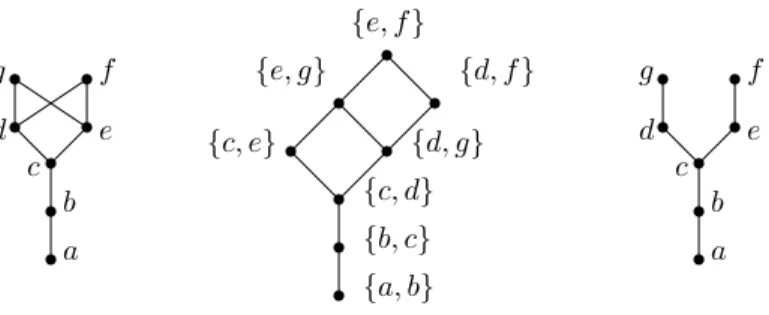
The statement of theorem 2.26 begs the question of whether all maximal chordal sub-graphs of a cocomparability graph are interval subsub-graphs. As shown in Figure 6 this is not the case. This naturally leads to the question: what is the complexity to compute a maximum interval subgraph (i.e., having a maximum number of edges) of a cocomparability graph? Unfortunately it has been shown in [12] that it is NP-hard.
It is interesting to compare theorem 2.26 to a result implicit in [20] but stated in [35] that says the following: every minimal triangulation (or chordalization) of a cocompara-bility graph is an interval graph. As a corollary, treewidth and pathwidth are equal for cocomparability graphs.
a b c d g e f {a, b} {b, c} {c, d} {d, g} {d, f} {c, e} {e, g} {e, f} a b c d g e f
Figure 6: From left to right: a cocomparability graph, along with one of its lattices and a maximal
chordal subgraph that is not an interval graph since it contains an asteroidal triple (a, f, g).
3
Algorithmic aspects
The problem of finding a maximal chordal subgraph of an arbitrary graph has been studied in [11] and an algorithm with complexity O(nm) has been proved. In this section, using a new graph search we will improve this to O(n + mlogn) for cocomparability graphs.
3.1
Graph searches and cocomparability graphs
In the introduction we presented two problems on cocomparability graphs solvable by graph searching where these algorithms are very similar to a corresponding algorithm on interval graphs. In subsection 3.2 we present other problems where this “lifting” technique provides new easily implementable cocomparability graph algorithms. All of the algorithms that we mention use a technique called the “+ tie-break rule” in which a total ordering τ of V (G)
is used to break ties in a particular graph search S. In particular, the next chosen vertex
in S will be the rightmost tied vertex in τ. Such a tie-breaking search will be denoted
S+(τ ). Many of these examples use that fact that some searches (most notably LDFS)
when applied as a “+-sweep” to a cocomp ordering produce a vertex ordering that is also a cocomp ordering. In fact, in [6] there is a characterization of the graph searches that have this property of preserving a cocomp ordering. Given a cocomparability graph G, computing a cocomp ordering can be done in linear time, [30]. This algorithm, however, is quite involved and other algorithms with a running time in O(n+m log(n)) are easier to implement [30, 19]. It should be noticed that up to now, it is not known if one can check if an ordering is a cocomp ordering in less than boolean matrix multiplication time.
3.2
Other examples of graph searches on cocomparability graphs
Following the two examples presented in the introduction we now present three other exam-ples of search based algorithms for other problems on cocomparability graphs:
vertex of an arbitrary LBFS starting at x. Then{x, y} forms a dominating pair in the sense that for all [x, y] paths in G, every vertex of G is either on the path or has a
neighbor on the path [7].4
• Let σ be an LDFS cocomp ordering of graph G. Then a simple dynamic programming algorithm for finding a longest path in an interval graph also solves the longest path problem on cocomparability graphs where σ is part of the input to the algorithm [32]. • Let σ be an LDFS cocomp ordering of graph G. Then a simple greedy algorithm for finding the maximum independent set (MIS) in an interval graph also solves the problem on cocomparability graphs where σ is part of the input to the algorithm [6].
It is well known that for any graph G = (V (G), E(G)) with MIS X ⊆ V (G), the set
Y = V (G)\ X forms a minimum cardinality vertex cover (i.e., every edge in E(G) has
at least one endpoint in Y ). The MIS algorithm in [6] certifies the constructed MIS by constructing a clique cover (i.e., a set of cliques such that each vertex belongs to exactly one clique in the set) of the same cardinality as the MIS. Recall that cocomparability graphs are perfect.
The last two algorithms in the list as well as the two in the introduction suggest the existence of an interesting relationship between interval and cocomparability graphs. We
believe that the basis of this relationship is the lattice MA(P ), which characterizes
cocom-parability graphs and shows that a cocomcocom-parability graph can be seen as a composition of
interval graphs (i.e., the maximal chains of cliques ofMA(P )).
3.3
Computing interval subgraphs of a cocomparability graph
In this section, we develop an algorithm that computes a maximal chain of the lattice
MA(Pσ) and show that it forms a maximal interval and chordal subgraph. The problem of
finding a maximal interval subgraph is the dual of the problem of finding a minimal interval completion (see [9, 23]). The algorithm that we are going to present uses a new graph search that we call LocalMNS, since it shares a lot of similarities with MNS.
This algorithm also gives us a way to compute a minimal interval extension of a partial order. An interval extension of a partial order is an extension that is also an interval order.
In [21, 22], it has been proved that the maximal chains of MA(P ) are in a one-to-one
correspondence with the minimal interval extensions. Therefore, our algorithm also allows us to compute a minimal interval extension of a partial order in O(n + mlogn) time.
This section is organized as follows. First we present a greedy algorithm, called Chain-clique with input a total ordering of an arbitrary graph’s vertex set, that computes an interval subgraph. This idea has already been described in [8] for extracting the maximal cliques of an interval graph from an interval ordering. Here we generalize it in order to accept as input any graph and any ordering. In subsection 3.4, we present a new graph search named
4In fact this result was proved for the larger family of asteroidal triple-free (AT-free) graphs and was the
LocalMNS. We will also prove that applying algorithm Chainclique on a LocalMNS cocomp
ordering produces a maximal chain of MA(P ). In subsection 2.4, we have shown that such
a maximal chain of MA(P ) forms a maximal interval and chordal subgraph.
Definition 3.1. Let G = (V (G), E(G)) be a graph and σ an ordering of V (G).
A graph H = (V (G), E(H)) with E(H)⊆ E(G) is a σ-maximal interval subgraph for the
ordering σ if and only if σ is an interval ordering for the graph H and∀S ⊆ E(G) − E(H),
S 6= ∅, σ is not an interval ordering for the graph H0 = (V (G), E(H)
∪ S).
Algorithm 1: Chainclique(G, σ)
Data: G = (V (G), E(G)) and a vertex ordering σ
Result: a chain of cliques C1,...,Cj
j ← 0;
i← 1;
C0 ← ∅;
while i≤ |V | do
j ← j + 1 %{Starting a new clique}%;
Cj ← {σ(i)} ∪ (N(σ(i)) ∩ Cj−1);
i← i + 1;
while i≤ |V | and σ(i) is universal to Cj do
Cj ← Cj∪ {σ(i)} %{Augmenting the clique}%;
i← i + 1;
Output C1, . . . , Cj;
As we will prove, Chainclique(G, σ) computes a σ-maximal interval subgraph for an arbitrary given graph G. To this end, Chainclique(G, σ) computes a sequence of cliques that respects the consecutiveness condition. Chainclique(G, σ) tries to increase the current clique and when it cannot, it creates a new clique and sets it to be the new current clique.
Another way to see it is that Chainclique(G, σ) discards all the edges xz ∈ E(G) such that
∃y, x <σ y <σ z and xy /∈ E(G).
It should be noticed that the cliques produced by Chainclique(G, σ) are not
necessar-ily maximal ones, for example take a P3 on the 3 vertices u, v, w with the edges uv
and vw. Chainclique(P3, σ) with σ = u, w, v, produces the cliques: {u}, {w, v}. It
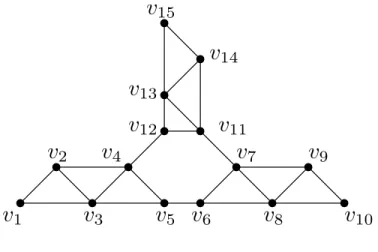
should also be noted that the algorithm works on an arbitrary graph and with an arbi-trary ordering. For an example, let us consider the graph H of Figure 7 and the ordering τ = v1, v2, v3, v4, v5, v6, v7, v8, v9, v10, v11, v12, v13, v14, v15. Chainclique(H, τ ) outputs
{v1, v2, v3}, {v2, v3, v4}, {v3, v4, v5}, {v5, v6}, {v6, v7, v8}, {v7, v8, v9}, {v8, v9, v10},
{v11, v12, v13}, {v11, v13, v14}, {v13, v14, v15}. For the graph H presented in Figure 7,
v
1v
2v
3v
4v
5v
6v
7v
8v
9v
10v
11v
12v
13v
14v
15Figure 7: The graph H
Now let us prove that Chainclique(G, σ) allows us to obtain a maximal interval subgraph for an ordering σ. The proof is organized as follows. In the first proposition we prove that Chainclique(G, σ) outputs a sequence of cliques that respects the consecutiveness property. In the second proposition, we prove that the ordering given to Chainclique is an interval ordering for the sequence of cliques. In the last proposition we prove that the graph formed by the sequence is a maximal interval subgraph for the ordering.
Proposition 3.2. For a graph G and an ordering σ, Chainclique(G, σ) outputs a sequence
of cliques C = C1, . . . , Ck such that for every Ce, Cf, Cg, 1≤ e ≤ f ≤ g ≤ k, Ce∩ Cg ⊆ Cf.
Proof. We do the proof by induction on the cliques ofC and the induction hypothesis is that
at each step j if x ∈ Cj−1-Cj then x /∈ Cj0, j0 ≥ j. Since C0 =∅, the hypothesis is true for
the initial case, j = 1.
Assume that the hypothesis is true for the first j ≥ 1 cliques. When we start to build
the clique Cj+1, we add a vertex that has not been considered before and its neighborhood
in Cj. By doing so, we cannot add a vertex x to Cj+1 such that x∈ Ci-Cj and i < j. When
we increase the clique, we only add vertices that have not been considered before and so
we cannot add a vertex x such that x ∈ Ci-Cj and i < j, in Cj+1. Therefore the induction
hypothesis is also verified at step j + 1.
Therefore using the characterization of interval graphs of corollary 2.22, Chainclique(G, σ) outputs a sequence of cliques that defines an interval subgraph.
Proposition 3.3. For a graphG and an ordering σ, Chainclique(G, σ) outputs a sequence of
cliques C = C1, . . . , Ck such that σ is an interval ordering for GC and ∀x ∈ Ci-Cj, ∀y ∈ Cj
-Ci, i < j, x <σ y.
Proof. Assume for contradiction that σ is not an interval ordering for GC. So there exists
appears, Cv be the first clique in which v appears and Cuw the first clique that contains both
u and w. Because Chainclique(G, σ) considers the vertices in the order they appear in σ,
the clique Cu must appear inC before the clique Cv. Using the same argument the clique Cv
must appear before the clique Cuw. But now Cu, Cv, Cuw contradict proposition 3.2, since
u /∈ Cv.
Now assume for contradiction that ∃x ∈ Ci-Cj, ∃y ∈ Cj-Ci, i < j, y <σ x. Now the
vertices are considered by Chainclique(G, σ) in the order they appear in σ. Since y <σ x,
let Cg be the first clique in which y appears. We see that g ≤ i. Since y belongs to Cg and
Cj, using proposition 3.2 we know that y ∈ Ci. Therefore y /∈ Cj-Ci, which contradicts our
choice of y. Thus ∀x ∈ Ci-Cj, ∀y ∈ Cj-Ci, i < j, x <σ y.
We are ready to prove that the graph formed by the sequence is a σ-maximal interval subgraph.
Proposition 3.4. For a graph G and an ordering σ, Chainclique(G, σ) outputs a sequence
of cliques C = C1, . . . , Ck that induces a maximal interval subgraph for the ordering σ.
Proof. Assume for contradiction that C = C1, . . . , Ck does not form a σ-maximal interval
subgraph. Therefore there exists a non empty set of edges S such that σ is an interval
ordering for the graph H = (V (G), E(C) ∪ S). Let uv be an edge of S and assume without
loss of generality that u <σ v. Let Ci be the last clique of C containing u and consider w
the first vertex of Ci+1, as chosen by Chainclique; clearly uw /∈ E and thus w 6= v. Now
u <σ w <σ v contradicts σ being an interval ordering for the graph H.
Proposition 3.5. Chainclique(G, σ) has complexity O(n + m).
Proof. All the tests can be performed by visiting once the neighborhood of a vertex. Since
the sequence of cliques forms a subgraph of G, its size is bounded by m. Therefore,
Chainclique(G, σ) has complexity O(n + m).
3.4
Computing a maximal chain in the lattice
In this subsection, we introduce a new graph search that will be used as a preprocessing
step in the computation of a maximal chain of MA(P ). This graph search will be called
LocalMNS and when we use Chainclique(G, σ) on a LocalMNS cocomp ordering σ we will
obtain a maximal chain of MA(P ).
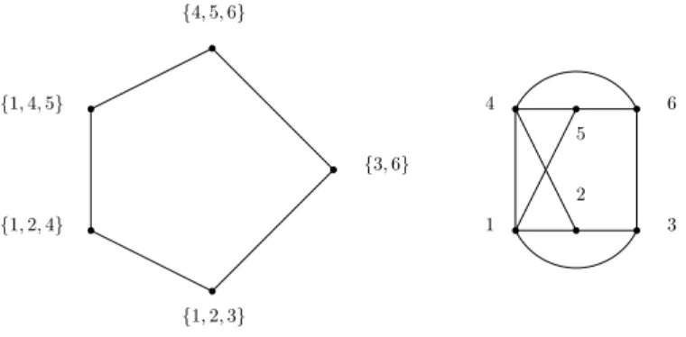
First, we start by looking at the behavior of Chainclique(G, σ) in which σ is a LBFS or a LDFS ordering. Let us consider the graph in Figure 8. Applying the algorithm Chainclique(G, σ) on the LDFS ordering σ = 1, 3, 2, 4, 6, 5, we get the chain of cliques {1, 2, 3}, {1, 2, 4} and {4, 5, 6} which is not a maximal chain of MA(P ). A similar re-sult holds using the LBFS ordering τ = 2, 3, 1, 4, 6, 5. Thus, LBFS and LDFS do not help
us find a maximal chain of cliques of MA(P ) using Chainclique(G, σ). This motivates the
{4, 5, 6} {1, 4, 5} {1, 2, 4} {3, 6} {1, 2, 3} 4 6 5 2 3 1
Figure 8: MA(P ) and the corresponding cocomparability graph G
Algorithm 2: LocalMNS
Data: G = (V, E)
Result: a total ordering σ such that σ(i) is the i’th visited vertex
D1 ← ∅;
V0
← V %{V0 is the set of unchosen vertices
}%;
X ← ∅ %{X is the set of chosen vertices}%;
;
for i = 1 to |V | do
v is chosen as a vertex from V0 with maximal neighborhood in D
i; σ(i) ← v; V0 ← V0 − {v}; X ← X ∪ {v};
Di+1← {v} ∪ (N(v) ∩ Di); % Note: x∈ Di-Di+1 → x /∈ Dj, j > i%;
This algorithm is very similar to the standard Maximal Neighborhood Search (MNS) algorithm. The only difference is in LocalMNS we are considering the neighborhood of the
unvisited vertices only in Di, which can be a strict subset of X (the visited vertices) and in
the case of MNS we are considering the neighborhood in X. This is the reason for the name
LocalMNS. Let us look at the behavior of LocalM N S+ on the example of Figure 8. Let
τ = 5, 6, 4, 2, 3, 1 be a cocomp ordering. σ = LocalM N S+(G, τ ) = 1, 3, 2, 4, 5, 6 is a cocomp
ordering and Chainclique(G, σ) computes the maximal chain{1, 2, 3}, {1, 2, 4}, {1, 4, 5} and
{4, 5, 6}.
Proposition 3.6. LocalMNS can be implemented in linear time.
Proof. It is well known that MNS can be implemented in linear time via MCS. So we will use
a LocalMCS to compute LocalMNS. LocalMCS works the same ways as LocalMNS except
that at each step i, instead of choosing a vertex of maximal neighborhood in Di, we choose
To implement LocalMCS we use a partition refinement technique. We use an ordered
partition in which each part contains the vertices of V0 having a given degree in D
i. This
structure can be easily maintained when Di+1 is formed from Di. If a vertex x ∈ Di does
not appear in Di+1, then x /∈ Dj, j > i and thus, during the execution of LocalMCS, we visit
the neighborhood of each vertex at most 2 times. Therefore LocalMCS is in O(n + m).
Proposition 3.7. LocalMNS+(G, σ) can be implemented in O(n + mlogn).
Proof. As in the previous proposition LocalM N S+ can be implemented via LocalM CS+.
We will also use an ordered partition in which each part contains the vertices of V0 having a
given degree in Di. But each part has to be ordered with respect to σ. This is the bottleneck
of this algorithm. To handle this difficulty each part will be represented by a tree data structure. This leads to an algorithm in O(n+mlogn).
We now prove that Chainclique(G, σ) on a LocalMNS cocomp ordering outputs a maximal chain of cliques. Let G be a cocomparability graph and τ a cocomp ordering of G. The proof
is organized as follows. We first show that σ = LocalM N S+(G, τ ) is a cocomp ordering.
Then we describe the structure of a maximal chain ofMA(Pσ) and its relation to Pσ. Finally
we prove that Chainclique(G, σ) outputs a maximal chain of MA(Pσ).
Lemma 3.8. If G is a cocomparability graph, then τ is a cocomp ordering if and only if
σ = LocalM N S+(G, τ ) is a cocomp ordering.
Proof. Note that this lemma can be stated as a corollary of the characterization in [6] of the
searches that preserve being a cocomp ordering. Instead we give a direct proof.
First we show that σ and τ satisfy the “flipping property” insofar as two nonadjacent vertices u, v must be in different relative orders in the two searches. To prove this, we assume
that u <σ v and u <τ v where, without loss of generality, u is the leftmost vertex in σ that
has such a non flipping non neighbor v. Now, because of the “+” rule in order for u <σ v
at the time u was selected by σ, there must exist a previously visited vertex w in σ such
that uw∈ E(G), vw /∈ E(G). Note that w <σ u <σ v. By the choice of u in σ, we see that
v <τ w and thus there is an umbrella u <τ v <τ w in τ , contradicting τ being a cocomp
ordering.
Now assume that τ is a cocomp ordering but σ is not. Let a <σ b <σ c be an umbrella
in σ where ac∈ E(G), ab, bc /∈ E(G). By the “flipping property”, b <τ a and c <τ b thereby
showing that c <τ b <τ a forms an umbrella in τ contradicting τ being a cocomp ordering.
The rest of the proof follows immediately.
Let us introduce some terminology to help us describe the behavior of Chainclique on an
ordering σ. Let ji be the first value of j such that σ(i) belongs to Cj (i.e., Cji is the leftmost
clique containing σ(i). Let C1
j, . . . , C lj
j be the sequence to build the clique Cj. Let pi be the