HAL Id: hal-02382427
https://hal.archives-ouvertes.fr/hal-02382427
Submitted on 3 Dec 2019HAL is a multi-disciplinary open access
archive for the deposit and dissemination of sci-entific research documents, whether they are pub-lished or not. The documents may come from teaching and research institutions in France or
L’archive ouverte pluridisciplinaire HAL, est destinée au dépôt et à la diffusion de documents scientifiques de niveau recherche, publiés ou non, émanant des établissements d’enseignement et de recherche français ou étrangers, des laboratoires
Sensitivity analysis of tree phenology models reveals
increasing sensitivity of their predictions to winter
chilling temperature and photoperiod with warming
climate
Julie Gaüzere, Camille Lucas, Ophélie Ronce, Hendrik Davi, Isabelle Chuine
To cite this version:
Julie GaÜzere, Camille Lucas, Ophélie Ronce, Hendrik Davi, Isabelle Chuine. Sensitivity analysis of tree phenology models reveals increasing sensitivity of their predictions to winter chilling tempera-ture and photoperiod with warming climate. Ecological Modelling, Elsevier, 2019, 411, pp.108805. �10.1016/j.ecolmodel.2019.108805�. �hal-02382427�
Title: Sensitivity analysis of tree phenology models reveals increasing sensitivity of their predictions to winter chilling temperature and photoperiod with warming climate
Authors: Gauzere J.1,2, Lucas C.1, Ronce O.2, Davi H.3, Chuine I.1
Adresses:
1CNRS, UMR 5175 CEFE-UM-UPVM3-EPHE-IRD, F-34293 Montpellier, France
2Institut des Sciences de l’Évolution, Université de Montpellier, CNRS, IRD, EPHE
Montpel-lier, France
3INRA, UR0629 URFM, F-84914 Avignon, France
Corresponding author: Julie Gauzere E-mail address: Julie.Gauzere@ed.ac.uk
Present address: Institute of Evolutionary Biology, School of Biological Sciences, University of Edinburgh, Charlotte Auerbach Road, Edinburgh EH9 3FL, UK.
Abstract
1
The phenology of plants is a major driver of agro-ecosystem processes and biosphere
feed-2
backs to the climate system. Phenology models are classically used in ecology and agronomy
3
to project future phenological changes. With our increasing understanding of the
environmen-4
tal cues affecting bud development, phenology models also increase in complexity. But, we
5
expect these cues, and the underlying physiological processes, to have varying influence on bud
6
break date predictions depending on the specific weather patterns in winter and spring. Here,
7
we evaluated the parameter sensitivity of state-of-the-art process-based phenology models that
8
have been widely used to predict forest tree species phenology. We used sensitivity analysis to
9
compare the behavior of models with increasing complexity under specific climatic conditions.
10
We thus assessed whether the influence of the parameters and modeled processes on predictions
11
varies with winter and spring temperatures. We found that the prediction of the bud break date
12
was mainly affected by the response to forcing temperature under current climatic conditions.
13
However, the impact of the parameters driving the response to chilling temperatures and to
pho-14
toperiod on the prediction of the models increased with warmer winter and spring temperatures.
15
Interaction effects between parameters played an important role on the prediction of models,
16
especially for the most complex models, but did not affect the relative influence of parameters
17
on bud break dates. Our results highlighted that a stronger focus should be given to the
char-18
acterization of the reaction norms to both forcing and chilling temperature to predict accurately
19
bud break dates in a larger range of climatic conditions and evaluate the evolutionary potential
20
of phenological traits with climate change.
21 22
Key words: Sensitivity analysis; Process-based modeling; Bud development; Forcing
1 Introduction
25
Bud break is a key phenological event that affects plant performance by defining the period
26
during which plants are able to grow, photosynthesize and produce their seeds. Therefore, the
27
phenology of plants is a major driver of agro-ecosystem processes (Cleland et al., 2007) and
28
biosphere feedbacks to the climate system (Richardson et al., 2013). It drives ecosystem
pro-29
ductivity (Richardson et al., 2012), carbon (Delpierre et al., 2009), water (Hogg et al., 2000)
30
and nutrient (Cooke & Weih, 2005) cycling processes, as well as energy balance (Wilson &
31
Baldocchi, 2000). Moreover, plant phenology critically affects yield and organoleptic quality
32
of crop harvest (Nissanka et al., 2015) as well as species distributions (Chuine, 2010). The
33
onset of plant activity has been reported to advance by 2.5 days per decade on average
dur-34
ing the last 50 years (Menzel et al., 2006), potentially increasing the risk of frost damages on
35
flowers and leaves (Vitasse et al., 2018a). These rapid responses have been shown to be highly
36
species-specific and are expected to have major consequences on species interactions, species
37
distributions, ecosystem functioning and forest carbon uptake (Cleland et al., 2007; Chuine,
38
2010; Richardson et al., 2013). Therefore, accurately predicting plant species phenology at
39
both large and local scales is of key importance for assessing the impact of global change on
40
agro-ecosystems and the multiple services they provide, as well as species range shift and
pop-41
ulations’ local extinction.
42 43
Fu et al. (2015b) showed however that the linear trend towards earlier spring onset had been
44
slowing down significantly during the last two decades. One of the hypothesis put forward by
45
the authors to explain this slowdown is the warming of winters. And indeed, recently, Asse
46
et al.(2018) documented the negative effect of the warming of winter on the leaf unfolding and
flowering date of several tree species. Air temperature is the major environmental factor
regu-48
lating the dates of budburst and flowering of plants (Rathcke & Lacey, 1985; Polgar & Primack,
49
2011). In perennial species, temperature has an antagonistic effect on bud development
depend-50
ing on the season: low temperature (called chilling) are required to release the endodormancy
51
of buds during winter, which is characterized by the inability of bud cells to growth despite
52
optimal growing conditions, while higher temperature (called forcing) are required to promote
53
bud cell elongation in spring. Recently, the effect of long photoperiod in compensating the lack
54
of chilling temperature has also been reported for some tree species (Laube et al., 2014; Way &
55
Montgomery, 2015; Zohner et al., 2016).
56 57
Our understanding of the environmental cues affecting species-specific bud break dates has
58
been increasing thanks to the compilation of large phenological datasets (Menzel et al., 2006; Fu
59
et al., 2015b), and to experimental work in controlled conditions using growth chambers (e.g.
60
Caffarra & Donnelly 2011; Zohner et al. 2016). This empirical knowledge has been essential
61
for the development and calibration of process-based phenology models (Chuine & Regniere,
62
2017), that are used to predict spring phenology over large spatial and temporal scales (e.g.
63
Chuine et al. 2016; Gauzere et al. 2017). While the relative contribution of environmental cues
64
in driving spring phenological responses in current and future climatic conditions is still debated
65
for most species (Chuine & Regniere, 2017; Laube et al., 2014; Fu et al., 2015a,b), the recent
66
declining of the response of spring onset to global warming suggests that the relative influence
67
of environmental cues driving the endodormancy phase varies with climatic conditions. Since
68
climate change is likely to generate non-equilibrium conditions, the relative influence of the
en-69
vironmental cues might also not remain constant over time. Overall, a strong expectation is that
environmental conditions. Yet, comprehensive analysis of the behavior of phenology models in
72
different climates are still lacking, while pioneer modeling studies in crops have shown that it is
73
expected to change depending on ecological conditions (e.g. Yin et al. 2005; Zhang et al. 2014).
74 75
Recently, Huber et al. (2018) highlighted the importance of improving our understanding
76
of models behavior, and identifying key parameters and processes that have the strongest
ef-77
fects on model predictions under different ecological conditions. It is a major stage to enhance
78
model applications across large spatial and temporal scales, as well as the robustness of model
79
projections. We embrace this view and acknowledge here the usefulness of sensitivity analysis
80
to reach this general objective. Sensitivity analyses are interesting statistical tools to address
81
the impact of parameters variations on the outputs of models (Cariboni et al., 2007), allowing
82
to evaluate both intrinsic (i.e. model structure and parameters) and extrinsic (i.e. model inputs)
83
sources of variation. They can also highlight model limitations and directions for further
im-84
provements (Saltelli et al., 2000; Cariboni et al., 2007). Therefore, they represent an important
85
step in the modeling cycle (Saltelli et al., 2000; Cariboni et al., 2007; Augusiak et al., 2014;
86
Courbaud et al., 2015).
87 88
For forest tree species, most studies in phenology modeling have focused on the analysis
89
of extrinsic sources of variation, e.g. investigating the uncertainty of climatic inputs on
sim-90
ulations (Morin & Chuine, 2005; Migliavacca et al., 2012). Ecological studies interested in
91
intrinsic sources of variation most often evaluate the effect of the variation of single parameters
92
on the model outputs, other parameters remaining fixed at a given default value (e.g. Lange
93
et al.2016). The major disadvantage of this approach is to neglect possible interactions among
94
parameters and to be unreliable in presence of non-linear relationships between the parameters
and the model predictions (Coutts & Yokomizo, 2014). At the opposite, sensitivity analyses
96
varying all parameters simultaneously allow to account for parameter interactions and
non-97
linear relationships and providing robust sensitivity measures for complex simulation models.
98
While phenology model complexity is increasing with our understanding of the physiological
99
responses involved in bud development, these interaction effects and non-linear relationships
100
can no more be overlooked. A first originality and aim of this study was thus to compare the
101
behavior of phenology models with increasing complexity, and to disentangle the main and
in-102
teraction effects of parameters on bud break date predictions.
103 104
The most commonly used phenology models are process-based, meaning that they describe
105
known or suspected cause-effect relationships between physiological processes and some
driv-106
ing factors in the organism’s environment to predict the precise occurrence in time of various
107
phenology events (see for review Chuine & Regniere 2017). The parameters of these models are
108
either defined using parameter values measured in experimental controlled conditions, or
statis-109
tically inferred from phenological and meteorological data using inverse modeling techniques.
110
Since they describe causal relationships derived from experimental work, the sensitivity
analy-111
sis of process-based models is supposed to reflect the sensitivity of the real processes (Saltelli
112
et al., 2000). Therefore, we can expect the sensitivity of phenology models to specific
param-113
eters, e.g. driving the endodormancy phase, to change with varying climatic conditions. The
114
impact of climate on observed and simulated bud break dates is expected to be complex,
be-115
cause of the cumulative and antagonistic effects of temperature depending on the season on bud
116
development (Chuine & Regniere, 2017). For this reason, we also aimed at testing the
param-117
eter sensitivity of phenology models to climatic conditions. We thus analyzed model behavior
or late bud break date. This study thus differ from that of Lange et al. (2016) which explored
120
the behavior of phenology models in uniformly warmer or colder conditions all along the year.
121
In the present study we used different observed climatically contrasted years with their specific
122
weather patterns.
123 124
Using a sensitivity analysis approach, we aimed at evaluating the parameter sensitivity of
125
state-of-the-art process-based phenology models that have been widely used to predict bud
126
break dates of forest tree species. The main originalities of this study are to (i) compare the
127
behavior of models with increasing complexity; and, (ii) perform this analysis under realistic
128
and contrasted climatic conditions in order to better estimate how the relative influence of
pa-129
rameters on model prediction varies with specific weather patterns in winter and spring. To
130
perform this study we used historical climatic conditions encountered at different elevations in
131
the Pyrenees Mountains, to cover a large range of temperature variation, without variation of the
132
day length between sites. More specifically, we propose here to: 1) evaluate whether increasing
133
model complexity is related to higher interaction effects between parameters; 2) identify key
134
parameters and processes that cause the highest variability in the output of the models under
135
different climatic regimes; 3) assess the physiological plausibility of this sensitivity; 4) discuss
136
our outcome for future studies that will use phenology models to address key question in
ecol-137
ogy and evolution. In particular, we expect parameters related to physiological responses to
138
spring forcing temperatures to have a stronger impact on the prediction of the bud break date
139
in cold environmental conditions, and more generally in historical climatic conditions in
West-140
ern Europe. On the opposite, we expect parameters related to endodormancy release (requiring
141
chilling conditions during winter) to have an increasing influence on the prediction of models in
142
warmer environmental conditions. Finally, we expect parameter interactions to have a greater
influence on the prediction of models with increasing model complexity.
144 145
2 Material and methods
146
2.1 Process-based phenology models
147
Process-based phenology models (see for review Chuine & Regniere 2017) are deeply grounded
148
on experimental results which have accumulated over the last 50 years and describe how the
de-149
velopment of buds, from dormancy induction in fall to bud break in spring, is determined by
150
the individual or interactive effects of different environmental cues, notably temperature and
151
photoperiod. Most of these models are based on the same framework (see Chuine & Regniere
152
2017). Each development phase (e.g. endodormancy, ecodormancy) is described by a
sub-153
model determining its reaction norms to various cues. Several response functions describing
154
the reaction norms to various cues can combine by addition, multiplication, or composition.
155
Development phases either are sequential (follow each other in time) or overlap (a phase can
156
start before the end of the previous one).
157 158
We chose three different kinds of model within this framework that represent the three main
159
types of environmental regulation of bud break (of either vegetative or reproductive buds) in
160
perennial species and are the most widely used in phenology studies: UniForc (Chuine, 2000),
161
UniChill (Chuine, 2000) and PGC (Gauzere et al., 2017). These models differ by their
com-162
plexity and by the environmental cues they account for. While UniForc and UniChill are
ther-163
mal ecodormancy and ecodormancy models respectively, PGC is a photothermal
endo-164
ecodormancy model. In the three models described below, t0defines the beginning of the
of forcing units to reach bud break.
167 168
UNIFORC- The UniForc model is an one-phase model, describing the cumulative effect of
169
forcing temperatures on the development of buds during the ecodormancy phase. This model
170
thus assumes that the endodormancy phase is always fully released and that there is no dynamic
171
effects of chilling and photoperiod on forcing requirements. Bud break occurs when the rate of
172
forcing, Rf (Eqn. 7), accumulated since t0, reaches the critical state of forcing F∗: 173
tf
∑
t0
Rf(T ) ≥ F∗ (1)
with T the daily average temperature.
174 175
UNICHILL– The UniChill model is a sequential two-phases model describing the
cumula-176
tive effect of chilling temperatures on the development of buds during the endodormancy phase
177
(first phase) and the cumulative effect of forcing temperatures during the ecodormancy phase.
178
Like in the Uniforc model, bud break occurs when the accumulated rate of forcing, Rf, reaches
179
F∗(Eqn. 1).
180
The start of the ecodormancy phase corresponds to the end of the endodormancy phase, tc,
181
which occurs when the accumulated rate of chilling Rc(Eqn. 8) has reached the critical state of
182 chilling C∗: 183 tc
∑
t0 Rc(T ) ≥ C∗ (2)PGC – The PGC model has been designed to explain bud break date of photosensitive
184
species, which might represent about 30 % of the species (Zohner et al., 2016). It has been
shown to be particular relevant to simulate the bud break date of beech (Fagus sylvatica) which
186
is one of the most photosensitive species for bud break (Gauzere et al., 2017). This is a
pho-187
tothermal model that integrates the compensatory effect of photoperiod on insufficient chilling
188
accumulation through a growth competence function (GC; Gauzere et al. 2017). The growth
189
competence function describes the ability of buds to respond to forcing temperatures. It
modu-190
lates the rate of forcing (Rf) through a multiplicative function to define the actual daily forcing
191
units accumulated by the bud until bud break as:
192
tf
∑
t0
(GC(P)Rf(T )) ≥ F∗ (3)
with P and T the daily photoperiod and average temperature respectively.
193 194
The growth competence (GC) is related to the daily photoperiod through a sigmoid function:
195
GC(P) = 1
1 + e−dP(P−P50(t)) (4)
with P50the mid-response photoperiod and dP the positive slope of the sigmoid function.
196
P50 is not constant and depends on the state of chilling (CS): the greater the accumulated rate
197
of chilling, the shorter the mid-response photoperiod, i.e. buds become sensitive to shorter
198
photoperiod when they have accumulated chilling:
199
P50(CS) = (12 − Pr) +
2Pr
1 + e−dC(CS(t)−C50) (5)
with Pr the range boundaries of the parameter P50, so that P50 ∈ [12-Pr; 12+Pr], dC the
200
negative slope of the sigmoid function, and C50 is the mid-response parameter if the sigmoid
function, reflecting chilling requirements under short-day length.
202
Finally, chilling units accumulated as:
203 CS(t) = t
∑
t0 Rc(T ) (6) 204 205For the sake of comparison, the version of the models used for this study have the same type
206
of response functions to forcing and to chilling temperatures. The response function to forcing
207
temperature, Rf, was defined as a sigmoid function as it has been shown to be the most realistic
208
experimentally (Hanninen et al., 1990; Caffarra & Donnelly, 2011):
209
Rf(Td) = 1
1 + e−dT(Td−T50) (7)
with dT the positive slope and T50 the mid-response temperature of the sigmoid function.
210
We defined the rate of chilling, Rc, as a threshold function (Caffarra et al., 2011b):
211 Rc(Td) = 1 if Td < Tb 0 if Td ≥ Tb (8)
with Td, the mean temperature of day d and Tb, the threshold temperature (also called base
tem-212
perature) of the function.
213 214
As defined here, the UniForc model has 4 parameters (t0, dT, T50, F∗), the UniChill model
215
6 parameters (t0, Tb, C∗, dT, T50, F∗), the PGC model 9 parameters (t0, Tb, C50, Pr, dC, dP, dT, 216
T50, F∗; Table 1). 217
218
2.2 Model calibration and validation
219
In order to set up the sensitivity analysis design, we first calibrated and validated the studied
220
phenology models for three emblematic tree species in European forests: common beech (Fagus
221
sylvatica L.), sessile oak (Quercus petraea L.) and silver fir (Abies alba Mill.). These results
222
were used to (i) define the natural parameter variation among tree species (Table 1) and (ii)
223
identify contemporary climatic years that produced particularly early and late spring phenology
224
(Appendix D). The three models were parametrized for the three different species using
obser-225
vations of the bud break date in the Pyrenees and corresponding weather data from 2005 to 2012.
226 227
The phenology of several populations located at different elevations following the Gave and
228
Ossau valleys in the Pyrenees have been yearly monitored since 2005. The studied populations
229
ranged from 131 to 1604 m (9 sites) for beech, from 131 to 1630 m (13 sites) for oak, and from
230
840 to 1604 m (6 sites) for fir (for further details about these populations, see Vitasse et al.
231
2009). Data used for this study consisted in the bud break date (BBCH 9) monitored from 2005
232
to 2012 in these populations. Models were parametrized using daily weather data since 2004
233
from Prosensor HOBO Pro (RH/Temp, Onset Computer Corporation, Bourne, MA 02532) that
234
have been placed at the core of each monitored population (Vitasse et al., 2009). Day length was
235
calculated according to the latitude of the meteorological stations (see Caffarra et al. 2011a).
236
Using these datasets, the three studied models were parametrized for each species following
237
Gauzere et al. (2017). The models RMSE varied from 5.85 to 10 days, with mean RMSE of
238
6.28 for beech, 6.92 for oak, 9.39 for fir (Appendix C).
2.3 Sensitivity analysis
241
To perform the sensitivity analysis we sampled 1,000,000 parameters combinations for each
242
model, to fully capture each parameter space. To sample each parameter, we used beta
distri-243
butions for the slope parameter of the sigmoid functions (equations 4, 5 and 7) and uniform
244
distributions for other parameters (Appendix E). The beta distribution was chosen to account
245
for the fact that variations in shape parameters have differential effects on sigmoid responses
246
(variation in extreme shape values have a lowest impact on the global shape of the sigmoid
247
function). The bounds of the sampling distributions were defined according to two criteria: (i)
248
the sampled values needed to be biologically relevant, i.e. make sense according to the
empiri-249
cal knowledge about the physiological responses and the adjusted values for the three species,
250
and (ii) produce positioned dates, i.e. dates different from the last day of the year (DOY 6= 365).
251
Due to these constraints, all parameters do not have the same variance (coefficient of variation
252
ranging from 0.05 to 0.18). Appendix E details the parameter values adjusted for each species
253
in the parameter space explored for the sensitivity analysis.
254 255
Two different sensitivity indexes, describing the proportion of variance of the model’s output
256
Y (here bud break date) explained by the variation of a given parameter Xi, were calculated
257
from the "Sobol" and "Sobol-Jansen" methods implemented in the package "sensitivity" of the
258
R software. These two methods implement the Monte Carlo estimation of the variance-based
259
method for sensitivity analysis proposed by Sobol (1993). More precisely, these functions allow
260
estimating the first-order and total-effect indexes from the variance decomposition, sometimes
261
referred to as functional ANOVA decomposition. The first-order index is defined as:
Si=VarX i(EX∼i(Y |Xi)) Var(Y ) (9) with 263 n
∑
i=1 Si= 1 (Si> 0) (10)Y is the prediction and Xithe ith parameter of the model. The notation (X ∼ i) indicates the
264
set of all variables except Xi. The numerator represents the contribution of the main effect of Xi
265
to the variation in the output, i.e. the effect of varying Xialone, but averaged over variations in
266
other input parameters. Siis standardized by the total variance to provide the fractional
contri-267
bution of each parameter i.
268 269
And total-effect index as:
270
STi=
EX∼i(VarX i(Y |X∼i))
Var(Y ) = 1 −
VarX∼i(EX i(Y |X∼i))
Var(Y ) (11) with 271 n
∑
i=1 STi≥ 1 (STi> 0) (12)due to the interaction effect, e.g. Xi and Xj both counted in STi and ST j. STi thus measures
272
the contribution of Xi to the variation in the output, including all variances caused by its
inter-273
actions with any other input variables.
274 275
2.4 Climatic data used for the sensitivity analysis
276
To perform the sensitivity analysis, we used the climate simulated at different elevations, over
277
a gradient of 1000 m, for the period from 1956 to 2012, in order to explore a large range
278
of climatic conditions. To study the response of the models to realistic climate at different
279
elevations, we used measurements taken with local weather stations on three forest sites, at
280
627 m, 1082 m and 1630 m a.s.l., along the Gave valley (Prosensor HOBO Pro; Vitasse et al.
281
2009). As this weather dataset only covered the period from 2004 to 2012, we also used Météo
282
France measurements at other stations located close to these sites, and data from the SAFRAN
283
reanalysis on the points of the systematic grid located in the valley, to simulate the climate at
284
the forest sites over a larger period (1959-2012). The temperature data recorded with the local
285
HOBO sensors were linearly correlated to the climatic data derived by the SAFRAN model of
286
Météo France (Quintana-Segui et al., 2008) for the same period. Daily minimum and maximum
287
temperature data from 1960 to 2012 were generated based on the long-term SAFRAN outputs
288
using the following equation:
289
T(X ) = βt(X ) + αt(X ).TSAFRAN (13)
with X the targeted site, βt and αt the intercept and the slope of the linear regression
be-290
tween TSAFRANand THOBOfor the period 2004-2012. The coefficients used for this equation are
291
provided in Appendix A. Day length was calculated according to the latitude of the forest sites
292
(see Caffarra et al. 2011a).
293 294
Over this large simulated period, we chose three climatically contrasted years, that
corre-295
sponded to (1) a year with winter and spring mean temperatures close to their global mean over
the 1960-2012 period ("normal climatic year"; year 1966), (2) a year expected to produce early
297
spring phenology, i.e. with cooler winter and warmer spring temperatures than normal ("early
298
climatic year"; year 2011) and (3) a year expected to produce late spring phenology, i.e. with
299
warmer winter and cooler spring temperatures than normal ("late climatic year"; year 1975;
300
Table 2; Appendix B). We checked that the three years selected indeed generated early, average
301
and late bud break dates using the adjusted models for different tree species (Appendix D). This
302
range of climatic conditions allowed us to credibly investigate the impact of specific weather
303
patterns in winter and spring on the behavior of the models.
304 305
P arameter Models Description Units Species parameter range Sampling distrib ution t0 UniF orc starting date of ecodormanc y DO Y [22; 90] U [-31; 92] t0 UniChill, PGC starting date of endodormanc y DO Y [-120; -62] U [-122; -31] F ∗ UniF orc, UniChill, PGC critical state of forcing DU [16.3; 106.8] U [1; 30] T50 UniF orc, UniChill, PGC mid-response temperature to forcing ◦ C [2.8; 15.7] U [0; 14] dT UniF orc, UniChill, PGC slope of the forcing response DR/ ◦ C [0.051; 0.44] B{α = 20; β = 1 .3 } C ∗ UniChill critical state of chilling DU [1.1; 116.7] U [1; 60] Tb UniChill, PGC threshold chilling temperature ◦ C [10.7; 14.9] U [7; 13] C50 PGC mid-response parameter of the photoperiod sensiti vity DU [5.7; 192.3] U [1; 60] Pr PGC range boundaries of the mid-response photoperiod hours [0.9; 1.5] U [1; 6] dC PGC slope of photoperiod sensiti vity response hours/units [-40; -0.64] B{α = 20; β = 1 .3 } [-10;-10 − 5 ] dP PGC slope of the gro wth competence DR/hours [0.26; 11.9] B{α = 20; β = 1 .3 } [10 − 5 ; 10] T able 1: Description and sampling distrib ution of the parameters of the three models used to perform the sensiti vity analysis. F or all parameters, except slope parameters, v alues were dra wn in uniform distrib utions U . F or slope parameters d , v alues were dra wn in be ta distrib utions B{α = 20; β = 1 .3 } . The species paramete r range pro vides the v ariation range of the adjusted parameters for three major European tree species (F . sylvatica , Q. petr eae , A. alba ). More details about the sampling distrib utions choices, based on the model calibration and the empirical kno wledge of about the ph ysiological responses, are pro vided in Appendix E). DO Y = day of the year; DU = de v elopmental units; DR = de v elopmental rate.
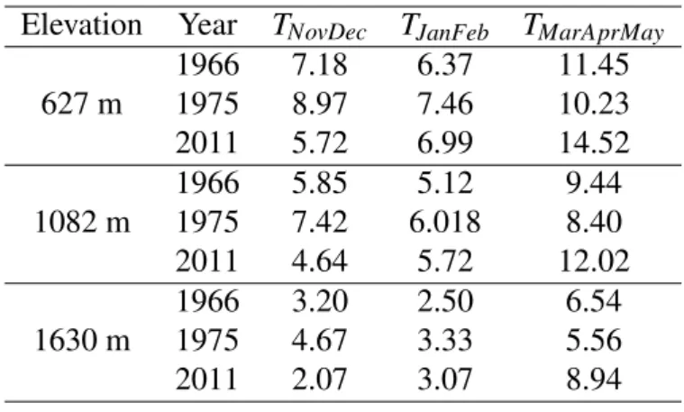
Elevation Year TNovDec TJanFeb TMarAprMay 1966 7.18 6.37 11.45 627 m 1975 8.97 7.46 10.23 2011 5.72 6.99 14.52 1966 5.85 5.12 9.44 1082 m 1975 7.42 6.018 8.40 2011 4.64 5.72 12.02 1966 3.20 2.50 6.54 1630 m 1975 4.67 3.33 5.56 2011 2.07 3.07 8.94
Table 2: Detail of the climatic conditions used to perform the sensitivity analysis of the
phe-nological models. With TNovDec the average temperature of November and December of the
previous year (in ˚ C), TJanFeb the average temperature of January and February of the focal
year (in ˚ C) and TMarAprMaythe average temperature of March, April and May of the focal year
3 Results
306
3.1 Main trends in parameter sensitivity of phenology models
307
For the three models, the mid-response temperature during the ecodormancy (T50) had the
great-308
est influence on the predictions of the models in most of the climatic conditions explored, except
309
in the cool winter-warm spring conditions producing early phenology (Figure 1, and see
Ap-310
pendices F, G and H for detailed results). This strong influence is both due to the main effect of
311
T50and its interaction with other parameters, and especially with dT, T50xdT defining the shape
312
of the forcing response during the ecodormancy phase. Under the conditions producing early
313
phenology, the main parameters affecting the predicted bud break date were t0, T50 and F∗ for
314
UniForc, UniChill and PGC respectively (Figure 1a). Note that the influence of the parameters
315
on the predictions of the models was significantly affected by their coefficient of variation (i.e.
316
parameters that had the highest variation also had the highest influence; Figure 2). However,
317
this effect only explained a small proportion of the total variation in the total-effect of the
pa-318
rameters (R2= 0.29).
319 320
3.2 The sensitivity to model parameters varies with model complexity
321
The sensitivity of model predictions to the variation in model parameters highly depended on
322
the phases and processes modeled (Figure 1). Predictions of the ecodormancy model UniForc
323
were more sensitive to the t0 parameter, i.e. the model starting date, than the predictions of
324
the endo-ecodormancy models UniChill and PGC, particularly under the climatic conditions
325
producing early phenology (Figure 1a and b). Predictions of the thermal model UniChill were
326
more sensitive to the critical amount of chilling to release dormancy (C∗ parameter) than the
predictions of the photothermal model PGC to the equivalent parameter (C50). Predictions of 328
this latter photothermal model was more sensitive to the critical amount of forcing (F∗) than
329
that of the thermal models UniForc and UniChill. Finally, predictions of the UniChill model
330
were more sensitive to the mid-response temperature during ecodormancy (T50) than that of the
331
UniForc and PGC models, which presented similar sensitivity to this parameter (Figure 1).
332
Depending on the model complexity, the uncertainty in the predictions will thus reply in the
333
accurate calibration of different key parameters.
334 335
3.3 The sensitivity to model parameters varies with climate
336
The sensitivity of the model predictions to the variation in model parameters also changed
ac-337
cording to the climatic conditions experienced during winter and spring (Figure 3). In the three
338
models, the sensitivity of the predictions to the mid-response temperature during ecodormancy
339
(T50) decreased with warming temperature (Figure 3), while the sensitivity to the parameters
340
driving the endodormancy phase (e.g. t0 in the UniForc model, C∗ in the UniChill model, dP
341
and C50 in the PGC model) increased with warming temperature (Figure 3). The sensitivity of
342
the endo-ecodormancy models to the critical amount of forcing to reach bud break (F∗) was
343
also higher in warmer conditions. This is probably because, even if forcing accumulation
be-344
comes less limiting with warming temperature, F∗still represents the minimum duration of the
345
ecodormancy phase and thus strongly drives bud break date.
346 347
The sensitivity of the predictions of the PGC model to both the critical amount of chilling
348
(C50) and the parameter determining the sensitivity to photoperiod (dP) increased with warming
the photoperiod related parameter was higher than that to chilling related parameters (C50 and 351
Tb; Figure 3). Finally, the sensitivity of PGC model predictions to the starting date of
endodor-352
mancy (t0) tended to increase with warming temperature conditions, while that of the Unichill
353
model remained constant and low (Figure 3). This result may be explained by the differences
354
in growth competence modeling between these two models. The growth competence function
355
of the PGC model is not null in autumn but decreases with the decreasing day length, and
in-356
duces endodormancy. If temperature conditions are particularly favorable, some forcing units
357
can be accumulated before endodormancy is fully induced contrary to the Unichill model. This
358
therefore gives an increasing importance to t0in driving bud break dates in warmer temperature
359
conditions.
360
For the three models, the increasing influence of the endodormancy vs ecodormancy related
361
parameters on bud break date predictions can already be noticed in warm winter conditions.
362 363
3.4 Main and interaction effects
364
In the results above, we describe the influence of the parameters on the predictions of the
mod-365
els based on their total effect, which include both main and second-order interaction effects.
366
However, it is also interesting to decompose these effects to understand their relative
contribu-367
tions to the variation of bud break dates. For most parameters, the total effects were mainly due
368
to main (or first-order) effects, and in a lesser extend to interaction effects between parameters
369
(or second-order effects; Figures 1). Second-order effects always explained less than 15 % of
370
the predictions variation (while the largest first-order effect explained more than 50 % of the
371
output variation ; Figure 4 and Appendix I). Interestingly, interaction effects did not modify the
372
relative influence of the parameters on the predictions of the models (Figures 1). Nevertheless,
total interaction effects represented an important source of variation in the predicted bud break
374
dates (Figure 4), in particular for the most complex models.
375 376
The total influence of interaction effects on model predictions also varied with the specific
377
weather patterns in winter and spring. For UniForc, total interaction effects were found to be
378
more important in the warm winter-cool spring conditions, producing late phenology, while for
379
PGC, these effects were more important in the cool winter-warm spring conditions, producing
380
early phenology (Figure 4a and c). The interaction between the parameters T50 and dT had the
381
largest effect on the predicted bud break date, notably in the coldest temperature conditions
382
(dTxT50; Appendices I). These two parameters define the shape of the response to
temper-383
ature during ecodormancy in the three models. For the PGC model in the warmest climatic
384
conditions, the interaction between the endodormancy starting date (t0) and the photoperiod
385
sensitivity (dP) also had an impact on the predicted bud break date (t0xdP; Appendix I).
386
The influence of interaction effects thus tended to increase with model complexity, but also
387
varied with specific weather patterns in winter and spring.
0.0 0.2 0.4 0.6 0.8 ● ● ● ● 0.0 0.2 0.4 0.6 0.8 main effect total effect a. Early conditions Par ameter effect t0 dT T50 F* UniFor c model 0.0 0.2 0.4 0.6 0.8 ● ● ● ● 0.0 0.2 0.4 0.6 0.8 main effect total effect t0 dT T50 F* c. Late conditions 0.0 0.2 0.4 0.6 0.8 ● ● ● ● 0.0 0.2 0.4 0.6 0.8 main effect total effect Parameters t0 dT T50 F* 0.0 0.2 0.4 0.6 0.8 ● ● ● ● ● ● 0.0 0.2 0.4 0.6 0.8 main effect total effect Par ameter effect t0 Tb dT T50 C* F* 0.0 0.2 0.4 0.6 0.8 ● ● ● ● ● ● 0.0 0.2 0.4 0.6 0.8 main effect total effect t0 Tb dT T50 C* F* 0.0 0.2 0.4 0.6 0.8 ● ● ● ● ● ● ● ● ● 0.0 0.2 0.4 0.6 0.8 main effect total effect Par ameter effect t0 Tb Pr dC dP dT T50 C50 F* 0.0 0.2 0.4 0.6 0.8 ● ● ● ● ● ● ● ● ● 0.0 0.2 0.4 0.6 0.8 main effect total effect t0 Tb Pr dC dP dT T50 C50 F* 0.0 0.2 0.4 0.6 0.8 ● ● ● ● ● ● ● ● ● 0.0 0.2 0.4 0.6 0.8 main effect total effect t0 Tb Pr dC dP dT T50 C50 F* UniChill m odel PGC model b. Sdt conditions 0.0 0.2 0.4 0.6 0.8 ● ● ● ● ● ● 0.0 0.2 0.4 0.6 0.8 main effect total effect t0 Tb dT T50 C* F* Parameters Parameters
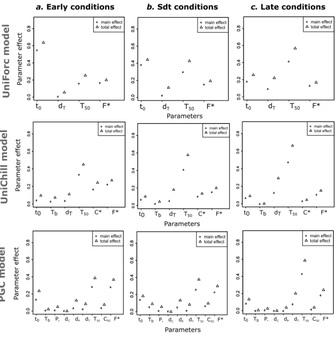
Figure 1: Main and total effects of the parameters on the predictions of the three studied models in the most contrasted climatic conditions. The main effect (or first-order effect)quantifies the individual effect of a parameter, i.e. without interactions. The total effect represents the first-and second-order effects (i.e. with second-order interaction effects). These effects quantify the proportion of variance of the model’s prediction explained by the variation of a given parame-ter. a. "Early conditions" corresponds to climatic conditions at 627 m in 2011, producing the earliest phenology, b. "standard conditions" to climatic conditions at 1082 m in 1966, produc-ing intermediate phenology, and c. "late conditions" to climatic conditions at 1603 m in 1975, producing the latest phenology over the range of conditions explored. The details of the results for each site and year are given in Appendix H.
0.06 0.08 0.10 0.12 0.14 0.16 0.18 0.0 0.1 0.2 0.3 0.4 0.5 0.6 Parameter CV Total ef fect (Sobo l index) R² = 0.29
Figure 2: Variation in the total-effect of parameters on the predictions of all models according to their coefficients of variation (CV). The coefficient of variation of each parameter was esti-mated from its sampling distribution. The R-squared was estiesti-mated using a linear model. The parameters with the highest CV were also the most influential on models prediction.
● ● ● ● ● ● ● ● ● 0.2 0.4 0.6 3 4 5 6 7 t 0 C* / C 50 Para meter ef fect ● ● ● ● ● ● ● ● ● 0.05 0.10 0.15 0.20 0.25 3 4 5 6 7 ● ● ● ● ● ● ● ● ● 0.3 0.4 0.5 0.6 7.5 10.0 12.5 T50 ● ● ● ● ● ● ● ● ● 0.15 0.20 0.25 0.30 0.35 0.40 7.5 10.0 12.5 F* ● ● ● ● ● ● ● ● ● 0.05 0.10 0.15 0.20 7.5 10.0 12.5 d P
average temperature January-February average temperature January-February
average temperature March-April-May average temperature March-April-May
average temperature March-April-May
Method ● PGC UniChill UniForc Para meter ef fect Para meter ef fect Para meter ef fect Para meter ef fect
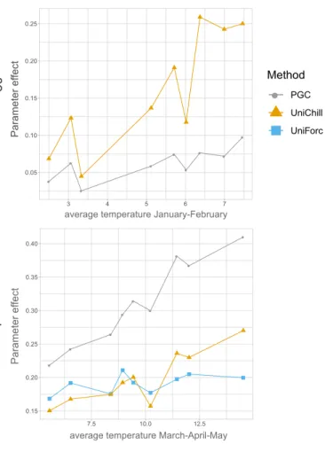
Figure 3: Variation in the total effect of the most biologically relevant parameters on the pre-dictions of the three studied models according to climatic variables (see also Appendix G). The total effect quantifies the proportion of variance in the model’s prediction explained by the vari-ation of a given parameter (considering its main and interaction effects). We chose to represent the average temperature of January and February because it is known to be involved in endodor-mancy release, and the average temperature of March, April and May because it is known to be involved in bud growth during ecodormancy. The climatic gradient corresponds to the nine contrasted climatic conditions used to perform the sensitivity analyses.
Main parameter effect Total interactions effects
UniForc model UniChill model PGC model
Parameter effects 0.0 0.1 0.2 0.3 0.4 0.5 0.6 0.0 0.1 0.2 0.3 0.4 0.5 0.6 0.0 0.1 0.2 0.3 0.4 0.5 0.6 c. Late conditions b. Standard conditions a. Early conditions
Figure 4: Proportion of the variation in model predictions explained by the main individual parameter effect and the total interaction effect for each model under the three most contrasted climatic conditions. The main parameter individual effects is the proportion of variance in the
predictions explained by the most influential parameter (T50in most cases). The total interaction
effects is the cumulative influence of the second-order interaction effects on models prediction. a. "Early conditions" corresponds to climatic conditions at 627 m in 2011, b. "standard condi-tions" to climatic conditions at 1082 m in 1966, and c. "late condicondi-tions" to climatic conditions at 1603 m in 1975.
4 Discussion
389
4.1 Bud break date predictions mainly depend on the forcing response under current
390
climatic conditions
391
The sensitivity analysis of the studied process-based models showed that the mid-response
tem-392
perature of the ecodormancy phase (called here T50) plays a critical role in the prediction of bud
393
break date under current climatic conditions. This result applies whether models account or not
394
for an endodormancy phase or a photoperiodic control of bud development. It therefore suggests
395
that the response to forcing temperature during the ecodormancy (defined by both T50 and dT in
396
the studied phenological models) is a major physiological response driving the variation of bud
397
break dates in temperate plant species in historical and current climatic conditions. This finding
398
is consistent with previous correlative modeling studies showing that bud break date variation
399
was mainly driven by the mean temperature of the two preceding months, which roughly
corre-400
sponds to the ecodormancy phase (e.g. Menzel et al. 2006). It is also consistent with previous
401
process-based modeling studies showing that models simulating only the ecodormancy phase
402
explained as much variance in bud break dates as models simulating both the endo- and
ecodor-403
mancy phases (Linkosalo et al., 2006; Gauzere et al., 2017). The similar performance of the
404
two types of model suggested either that the fulfillment of chilling requirements had not been
405
a limiting factor so far, or that the endodormancy phase is not accurately modeled (Linkosalo
406
et al., 2006; Chuine et al., 2016). Our results support the first hypothesis, i.e. winter chilling
407
temperature have played a minor role in bud break variations so far, which also explains why
408
the response of plant species to climate warming has so far resulted in an advancement of the
409
bud break dates (Menzel et al., 2006). A methodological consequence of this is that
phenolog-410
ical records in natural populations may not allow estimating accurately endodormancy model
parameters (Chuine et al., 2016).
412 413
4.2 Bud break date predictions are increasingly dependent on chilling temperatures and
414
photoperiod as climate warms
415
We found that the effect of the reaction norm to forcing temperature on the prediction of the
416
bud break date decreased with warming spring conditions, while the effect of chilling
accu-417
mulation during the endodormancy phase increased with warming winter temperature for the
418
thermal endo-ecodormancy models UniChill and PGC. This suggests that in warmer
environ-419
mental conditions reaction norms to temperature during both bud endodormancy and
ecodor-420
mancy are critical in determining bud break dates. This result is supported by several recent
421
experimental studies showing that temperature sensitivity of the bud break dates was currently
422
decreasing, likely due to an increasing influence of warming winters on bud endodormancy (Fu
423
et al., 2015a,b; Vitasse et al., 2018b; Asse et al., 2018). In particular, Vitasse et al. (2018b)
424
showed that a differential response to chilling temperatures between trees living at low and high
425
elevations may explain the difference in the temporal trends of bud break date advancement
426
observed at different elevations with warming conditions during the last decade. Overall, these
427
results highlight that the influence of chilling temperatures on bud development can no longer
428
be overlooked, and that the correct estimation of the parameters governing the endodormancy
429
phase is required to accurately predict bud break.
430 431
The sensitivity analysis of the photothermal endo-ecodormancy model PGC showed that the
432
influence of the photoperiodic response (through the dPparameter) on the prediction of the bud
that the phenology of up to 30 % of tree species might be sensitive to photoperiod at various
435
degrees (Laube et al., 2014; Zohner et al., 2016). Understanding how this increasing effect of
436
the photoperiodic cue will affect the variation of bud break dates in future climatic conditions
437
is an issue still debated (Fu et al., 2015b; Gauzere et al., 2017). However, in the most sensitive
438
species, such as beech, it has been suggested that this sensitivity may counteract the negative
439
effect of insufficient chilling during winter (Gauzere et al., 2017). Our results thus highlight
440
that a stronger focus should be given to the modeling of the reaction norm to photoperiod to
441
be able to accurately predict bud break dates of up to 30 % of tree species in future climatic
442
conditions.
443 444
4.3 Originality and limits of the study
445
Only a few studies have performed sensitivity analysis of phenology models so far. They
ei-446
ther analyzed the behavior of phenology models, identified the main sources of uncertainties in
447
bud break date predictions, or assessed the consequences of phenological uncertainties on
re-448
lated processes (e.g. Morin & Chuine 2005; Migliavacca et al. 2012; Zhang et al. 2014; Lange
449
et al.2016). A key results from these previous studies is that uncertainty in climate conditions,
450
notably generated by climate scenarios, was a greater source of variation in phenological date
451
projections than uncertainty in phenology models (Migliavacca et al., 2012).
452 453
To our knowledge, this study is the first to have compared the behavior of different
phenol-454
ogy models, with increasing complexity, and to perform this analysis under different weather
455
patterns in winter and spring. The results found here are in line with a recent sensitivity
anal-456
ysis of species-specific phenology models, which found an increasing importance of chilling
requirements and photoperiod in warm climatic conditions for temperate tree species (Lange
458
et al., 2016). The consistency of our results with the sensitivity analysis of other phenology
459
models strengthens the scope of our study, and thus further stress the importance of
investigat-460
ing the behavior of phenology models in contrasted climatic conditions in order to fully embrace
461
their robustness.
462 463
While the climate we used to perform the sensitivity analyses covers a small geographical
464
region, it still explores a large range of variation in winter and spring average temperatures
465
(TNovDec∈ [2.07; 8.97], TMarAprNay∈ [5.56; 14.52]). This temperature variation is less impor-466
tant then in other sensitivity analyses (e.g. Lange et al. 2016), but it is large enough to allow
467
extrapolating the results of this study at larger spatial scales. The aim of the present study was
468
not to investigate the behavior of phenology models under climate change scenarios.
Neverthe-469
less, by extrapolating our results on the impact of warming conditions on parameter sensitivity,
470
we can expect the influence of the parameters governing the endodormancy to overall have more
471
influence on bud break date predictions in the future.
472 473
Due to the high computational requirement of sensitivity analyses, most studies usually
ne-474
glect, partially or completely, interaction effects between model parameters as a source of output
475
variation (e.g. Lange et al. 2016). However, the complexity of process-based phenology models
476
tends to increase as we gain better knowledge about the physiological processes involved in bud
477
development. With increasing model complexity and realism, we can expect interaction effects
478
to have non-negligible influence on the prediction of the models, and thus local sensitivity
anal-479
ysis to partially reveal the effect of parameters on output variance. Our results also suggest that
effects. Moreover, increasing model complexity would generate higher uncertainty in model
482
outputs because of parameter compensation during the statistical adjustment, notably if models
483
are used to perform predictions outside of the range of the climatic conditions used to adjust
484
them (Gauzere et al., 2017).
485 486
Here, we showed that sensitivity analysis of process-based phenology models are relevant
487
to identify key parameters and processes that have the largest effect on phenology (Migliavacca
488
et al., 2012; Lange et al., 2016). However, the choice of the parameter variation range likely
489
affects the results of such analyses. Since for most plant species, the range limits or shape of the
490
distributions of the physiological parameters in natural populations are unknown, such
sensitiv-491
ity analyses rely on assumptions that cannot be tested. Here, we might have overestimated the
492
real contribution of T50 and F∗to the variation of the bud break date due to uneven variances in
493
parameter sampling distributions. This effect of parameter variation on the outcome of
sensitiv-494
ity analyses should be more acknowledged. To improve the scope and relevance of sensitivity
495
analyses, more attention should be given to the characterization of the natural variation of the
496
physiological parameters described in process-based models (e.g. Burghardt et al. 2015).
497 498
4.4 Implications for the adaptive potential of phenological traits
499
While the sensitivity analysis of phenology models has direct implications for ecological and
500
climate change studies, we wanted to highlight also here their usefulness for evolutionary
stud-501
ies. The bud break date is among the most genetically differentiated trait across species
dis-502
tribution ranges (De Kort et al., 2013), suggesting that it is strongly involved in the process of
503
local genetic adaptation. Evolutionary response of the bud break date is expected to depend on
which parameters present genetic variation and how this variation impacts the bud break date,
505
i.e.the expressed trait variation. Sensitivity analysis outputs can be used to address this second
506
issue. For example, our results show that the mid-response temperature of the ecodormancy
507
phase (T50) has the highest impact on the variation of the bud break date in most conditions.
508
We thus suggest that future experimental research consider measuring the genetic variation of
509
this key physiological trait in natural populations and crops to evaluate their adaptive potential.
510
This can be done by monitoring bud break of several genotypes either in varying controlled
511
conditions (e.g. Caffarra et al. 2011b), or by monitoring growth transcriptor factors in natura
512
or in the field using new transcriptomic technics (e.g. Nagano et al. 2012), or even better by
513
combining both approaches (e.g. Satake et al. 2013). Given the increasing importance of the
514
response to chilling temperatures during the endodormancy phase to determine the bud break
515
date in warming conditions, future experimental research might additionally consider
measur-516
ing the genetic variation in chilling requirement and reaction norms to chilling temperature,
517
especially in species requiring large amount of chilling. Finally, future experimental research
518
should consider measuring the genetic variation in the reaction norm to photoperiod in most
519
sensitive species, and notably beech (Goyne et al. 1989 for example in crops).
520 521
5 Conclusions
522
The identification of the physiological responses underlying the bud break date variation in
cur-523
rent environmental conditions is an important on-going experimental research field (Fu et al.,
524
2015a,b; Vitasse et al., 2018b). Assuming that process-based phenology models reflect real
525
physiological responses and processes, the analysis of their behavior under contrasted climatic
jor influence of the response to forcing temperature on the prediction of the bud break date,
528
but also an increasing importance of the responses to chilling temperature and photoperiod in
529
warming environmental conditions. Changes in the sensitivity of the prediction of phenology
530
models to their parameters with climatic conditions highlights that we need to better take into
531
account the temporal and spatial variation of environmental conditions when analyzing
pheno-532
logical changes (Vitasse et al., 2018b). More generally, we acknowledge here that the sensitivity
533
analysis of process-based models is a useful tool to understand the relative contributions of
envi-534
ronmental cues in driving phenotypic traits variation and their evolutionary potential (Donohue
535
et al., 2015; Burghardt et al., 2015; Lange et al., 2016).
536 537
Acknowledgements
538
We thank Claude Bruchou and Guillaume Marie for helpful discussions on the approach and
539
results of this manuscript. We thank also two anonymous reviewers for their constructive
com-540
ments which helped us improving previous versions of this article. This study was founded by
541
the ANR-13-ADAP-0006 project MeCC. The authors have no conflict of interest to declare.
References
543
Asse, D., Chuine, I., Vitasse, Y., Yoccoz, N.G., Delpierre, N., Badeau, V., Delestrade, A. &
544
Randin, C.F. (2018) Warmer winters reduce the advance of tree spring phenology induced by
545
warmer springs in the Alps. Agricultural and Forest Meteorology, 252, 220–230.
546
Augusiak, J., Van den Brink, P.J. & Grimm, V. (2014) Merging validation and evaluation of
547
ecological models to ‘evaludation’: A review of terminology and a practical approach.
Eco-548
logical Modelling, 280, 117–128.
549
Burghardt, L.T., Metcalf, C.J.E., Wilczek, A.M., Schmitt, J. & Donohue, K. (2015) Modeling
550
the Influence of Genetic and Environmental Variation on the Expression of Plant Life Cycles
551
across Landscapes. American Naturalist, 185, 212–227.
552
Caffarra, A. & Donnelly, A. (2011) The ecological significance of phenology in four different
553
tree species: effects of light and temperature on bud burst. International Journal of
Biomete-554
orology, 55, 711–721.
555
Caffarra, A., Donnelly, A. & Chuine, I. (2011a) Modelling the timing of Betula pubescens
556
budburst. II. Integrating complex effects of photoperiod into process-based models. Climate
557
Research, 46, 159–170.
558
Caffarra, A., Donnelly, A., Chuine, I. & Jones, M.B. (2011b) Modelling the timing of Betula
559
pubescens budburst. I. Temperature and photoperiod: a conceptual model. Climate Research,
560
46, 147–157.
561
Cariboni, J., Gatelli, D., Liska, R. & Saltelli, A. (2007) The role of sensitivity analysis in
eco-562
logical modelling. Ecological Modelling, 203, 167–182. 4th Conference of the
International-563
Society-for-Ecological-Informatics, Busan, SOUTH KOREA, OCT 24-28, 2004.
564
Chuine, I. (2000) A unified model for budburst of trees. Journal of Theoretical Biology, 207,
565
337–347.
566
Chuine, I., Bonhomme, M., Legave, J.M., Garcia de Cortazar, A., Charrier, G., Lacointe, A. &
567
Améglio, T. (2016) Can phenological models predict tree phenology accurately in the future?
568
the unrevealed hurdle of endodormancy break. Global Change Biology, 22, 3444–3460.
569
Chuine, I. (2010) Why does phenology drive species distribution? Philosophical Transactions
570
of the Royal Society B-Biological Sciences, 365, 3149–3160.
571
Chuine, I. & Regniere, J. (2017) Process-Based Models of Phenology for Plants and Animals.
572
Futuyma, DJ, ed., Annual Review of Ecology, Evolution, and Systematics, volume 48 of
573
Annual Review of Ecology Evolution and Systematics, pp. 159–182.
574
Cleland, E.E., Chuine, I., Menzel, A., Mooney, H.A. & Schwartz, M.D. (2007) Shifting plant
575
phenology in response to global change. Trends in Ecology & Evolution, 22, 357–365.
576
Cooke, J. & Weih, M. (2005) Nitrogen storage and seasonal nitrogen cycling in Populus:
bridg-577
ing molecular physiology and ecophysiology. New Phytologist, 167, 19–30.
Courbaud, B., Lafond, V., Lagarrigues, G., Vieilledent, G., Cordonnier, T., Jabot, F. & de
Col-579
igny, F. (2015) Applying ecological model evaludation: Lessons learned with the forest
dy-580
namics model Samsara2. Ecological Modelling, 314, 1–14.
581
Coutts, S.R. & Yokomizo, H. (2014) Meta-models as a straightforward approach to the
sensi-582
tivity analysis of complex models. Population Ecology, 56, 7–19.
583
De Kort, H., Vandepitte, K. & Honnay, O. (2013) A meta-analysis of the effects of plant traits
584
and geographical scale on the magnitude of adaptive differentiation as measured by the
dif-585
ference between Q(ST) and F-ST. Evolutionary Ecology, 27, 1081–1097.
586
Delpierre, N., Dufrene, E., Soudani, K., Ulrich, E., Cecchini, S., Boe, J. & Francois, C. (2009)
587
Modelling interannual and spatial variability of leaf senescence for three deciduous tree
588
species in France. Agricultural And Forest Meteorology, 149, 938–948.
589
Donohue, K., Burghardt, L.T., Runcie, D., Bradford, K.J. & Schmitt, J. (2015) Applying
de-590
velopmental threshold models to evolutionary ecology. Trends in Ecology & Evolution, 30,
591
66–77.
592
Fu, Y.H., Piao, S., Vitasse, Y., Zhao, H., De Boeck, H.J., Liu, Q., Yang, H., Weber, U.,
Han-593
ninen, H. & Janssens, I.A. (2015a) Increased heat requirement for leaf flushing in
temper-594
ate woody species over 1980-2012: effects of chilling, precipitation and insolation. Global
595
Change Biology, 21, 2687–2697.
596
Fu, Y.H., Zhao, H., Piao, S., Peaucelle, M., Peng, S., Zhou, G., Ciais, P., Huang, M., Menzel,
597
A., Uelas, J.P., Song, Y., Vitasse, Y., Zeng, Z. & Janssens, I.A. (2015b) Declining global
598
warming effects on the phenology of spring leaf unfolding. Nature, 526, 104+.
599
Gauzere, J., Delzon, S., Davi, H., Bonhomme, M., Garcia de Cortazar, A. & Chuine, I. (2017)
600
Integrating interactive effects of chilling and photoperiod in phenological process-based
mod-601
els. a case study with two european tree species: Fagus sylvatica and quercus petraea.
Agri-602
cultural and Forest Meteorology, 244, 9–20.
603
Goyne, P., Schneiter, A., Cleary, K., Creelman, R., Stegmeier, W. & Wooding, F. (1989)
Sun-604
flower genotype response to photoperiod and temperature in field environments. Agronomy
605
Journal, 81, 826–831.
606
Hanninen, H., Hakkinen, R., Hari, P. & Koski, V. (1990) Timing of growth cessation in relation
607
to climatic adaptation of northern woody-plants. Tree Physiology, 6, 29–39.
608
Hogg, E., Price, D. & Black, T. (2000) Postulated feedbacks of deciduous forest phenology on
609
seasonal climate patterns in the western Canadian interior. Journal of Climate, 13, 4229–
610
4243.
611
Huber, N., Bugmann, H. & Lafond, V. (2018) Global sensitivity analysis of a dynamic
vegeta-612
tion model: Model sensitivity depends on successional time, climate and competitive
inter-613
actions. Ecological Modelling, 368, 377–390.
614
Lange, M., Schaber, J., Marxn A. abd Jäckel, G., Badeck, F., Seppelt, R. & Doktor, D. (2016)
615
Simulation of forest tree species bud burst dates for different climate scenarios: chilling
616
requirements and photo-period may limit bud burst advancement. International Journal of
617
Biometeorology, DOI: 10.1007/s00484-016-1161-8.
Laube, J., Sparks, T.H., Estrella, N., Hoefler, J., Ankerst, D.P. & Menzel, A. (2014) Chilling
619
outweighs photoperiod in preventing precocious spring development. Global Change
Biol-620
ogy, 20, 170–182.
621
Linkosalo, T., Hakkinen, R. & Hanninen, H. (2006) Models of the spring phenology of boreal
622
and temperate trees: is there something missing? Tree Physiology, 26, 1165–1172.
623
Menzel, A., Sparks, T.H., Estrella, N., Koch, E., Aasa, A., Ahas, R., Alm-Kuebler, K., Bissolli,
624
P., Braslavska, O., Briede, A., Chmielewski, F.M., Crepinsek, Z., Curnel, Y., Dahl, A., Defila,
625
C., Donnelly, A., Filella, Y., Jatcza, K., Mage, F., Mestre, A., Nordli, O., Penuelas, J., Pirinen,
626
P., Remisova, V., Scheifinger, H., Striz, M., Susnik, A., Van Vliet, A.J.H., Wielgolaski, F.E.,
627
Zach, S. & Zust, A. (2006) European phenological response to climate change matches the
628
warming pattern. Global Change Biology, 12, 1969–1976.
629
Migliavacca, M., Sonnentag, O., Keenan, T.F., Cescatii, A., Keefe, J.O. & Richardson, A.D.
630
(2012) On the uncertainty of phenological responses to climate change, and implications for
631
a terrestrial biosphere model. Biogeosciences, 9, 2063–2083.
632
Morin, X. & Chuine, I. (2005) Sensitivity analysis of the tree distribution model PHENOFIT
633
to climatic input characteristics: implications for climate impact assessment. Global Change
634
Biology, 11, 1493–1503.
635
Nagano, A.J., Sato, Y., Mihara, M., Antonio, B.A., Motoyama, R., Itoh, H., Nagamura, Y. &
636
Izawa, T. (2012) Deciphering and Prediction of Transcriptome Dynamics under Fluctuating
637
Field Conditions. Cell, 151, 1358–1369.
638
Nissanka, S.P., Karunaratne, A.S., Perera, R., Weerakoon, W.M.W., Thorburn, P.J. & Wallach,
639
D. (2015) Calibration of the phenology sub-model of APSIM-Oryza: Going beyond goodness
640
of fit. Environmental Modelling & Software, 70, 128–137.
641
Polgar, C.A. & Primack, R.B. (2011) Leaf-out phenology of temperate woody plants: from
642
trees to ecosystems. New Phytologist, 191, 926–941.
643
Quintana-Segui, P., Le Moigne, P., Durand, Y., Martin, E., Habets, F., Baillon, M., Canellas, C.,
644
Franchisteguy, L. & Morel, S. (2008) Analysis of near-surface atmospheric variables:
Valida-645
tion of the SAFRAN analysis over France. Journal of Applied Meteorology and Climatology,
646
47, 92–107.
647
Rathcke, B. & Lacey, E. (1985) Phenological patterns of terrestrial plants. Annual Review of
648
Ecology and Systematics, 16, 179–214.
649
Richardson, A.D., Anderson, R.S., Arain, M.A., Barr, A.G., Bohrer, G., Chen, G., Chen, J.M.,
650
Ciais, P., Davis, K.J., Desai, A.R., Dietze, M.C., Dragoni, D., Garrity, S.R., Gough, C.M.,
651
Grant, R., Hollinger, D.Y., Margolis, H.A., McCaughey, H., Migliavacca, M., Monson, R.K.,
652
Munger, J.W., Poulter, B., Raczka, B.M., Ricciuto, D.M., Sahoo, A.K., Schaefer, K., Tian, H.,
653
Vargas, R., Verbeeck, H., Xiao, J. & Xue, Y. (2012) Terrestrial biosphere models need better
654
representation of vegetation phenology: results from the North American Carbon Program
655
Site Synthesis. Global Change Biology, 18, 566–584.
656
Richardson, A.D., Keenan, T.F., Migliavacca, M., Ryu, Y., Sonnentag, O. & Toomey, M. (2013)