Ferromagnetic/antiferromagnetic exchange bias nanostructures for ultimate spintronic devices

(1)

HAL Id: tel-01161786

https://tel.archives-ouvertes.fr/tel-01161786

Submitted on 9 Jun 2015

HAL is a multi-disciplinary open access archive for the deposit and dissemination of sci-entific research documents, whether they are pub-lished or not. The documents may come from teaching and research institutions in France or abroad, or from public or private research centers.

L’archive ouverte pluridisciplinaire HAL, est destinée au dépôt et à la diffusion de documents scientifiques de niveau recherche, publiés ou non, émanant des établissements d’enseignement et de recherche français ou étrangers, des laboratoires publics ou privés.

Ferromagnetic/antiferromagnetic exchange bias

nanostructures for ultimate spintronic devices

Kamil Akmaldinov

To cite this version:

Kamil Akmaldinov. Ferromagnetic/antiferromagnetic exchange bias nanostructures for ultimate spin-tronic devices. Condensed Matter [cond-mat]. Université Grenoble Alpes, 2015. English. �NNT : 2015GREAY009�. �tel-01161786�

(2)

THÈSE

Pour obtenir le grade de

DOCTEUR DE L’UNIVERSITÉ DE GRENOBLE

Spécialité : Physique

Arrêté ministériel : 7 août 2006

Présentée par

Kamil AKMALDINOV

Thèse dirigée par Vincent BALTZ codirigée par Bernard DIENY

préparée au sein du Laboratoire SPINTEC et de la société Crocus Technology

dans l'École Doctorale de Physique de Grenoble

Ferromagnetic/antiferromagnetic

exchange bias nanostructures

for ultimate spintronic devices

Thèse soutenue publiquement le 6 février 2015,

devant le jury composé de :

M. Manuel BIBES

Directeur de recherche du CNRS, Rapporteur

M. Robert STAMPS

Professeur de l’Université de Glasgow, Rapporteur

M. Olivier BOURGEOIS

Directeur de recherche du CNRS, Membre

M. Luc LECHEVALLIER

Maître de conférences de l’Université de Cergy-Pontoise, Membre

Mme Clarisse DUCRUET

Ingénieur R&D chez Crocus Technology, Membre

(3)

(4)

(5)

(6)

INTRODUCTION

The research presented here is focused on ferromagnetic/antiferromagnetic (F/AF) exchange bias (EB) nanostructures for ultimate spintronics devices and more specifically for the improvement of thermally-assisted random access memories (TA-MRAM) now developed by the CROCUS technology company. It was conducted within the SPINTEC laboratory (spintronics and technology of compounds), joint research unit between French institutions: University of Grenoble Alpes, CNRS, CEA (INAC) in the frame of a joint research and development program between the CROCUS technology company and the SPINTEC laboratory. Such a program financially supported this PhD thesis under a CIFRE grant (Convention Industrielle de Formation par la REcherche).

Basically, a MRAM comprises a magnetic tunnel junction, an exchange biased reference layer and a storage layer. The specificity of a TA-MRAM is that the storage layer is also exchange biased for improved data retention. The bit writing scheme of every memory cell involves additional heating to temporarily unblock the exchange bias coupling between the F and AF stacks of the storage layer. To ensure stable device functioning and to compete with other memory types the memory cell to memory cell parameters dispersion such as the exchange bias loop shift and the write power should be as low as possible. It is well-known, that EB can be strongly affected by diverse external conditions - from the deposition rates and layers thicknesses to annealing temperatures and fields. It becomes even more critical when talking about nano-dimensional structures, where the shape and the size of a bit also matters. No doubts, all these parameters should be taken into account to control the variability and in the literature there are numerous studies focused on shape, growth and fabrication reasons for cells dispersions. Apart from that, it is widely recognised that EB is strongly dependent on the F-AF interfacial quality and in particular on the amount of highly unstable regions - spin-glass like phases. It was supposed few years ago that randomly spread spin-glass like phases at the F/AF interface or within the bulk of the AF layer significantly contribute to the distributions of EB properties in devices after processing. This PhD thesis aimed at factually addressing this point. The manuscript is therefore structured as follows:

Chapter 1 introduces the exchange bias phenomenology and state-of-art. It covers early theoretical suggestions considering ideal systems and to more complicated systems accounting for interfacial spin-glass like phases. It continues with the description of nowadays macroscopic picture based on both experimental findings and theoretical view.

(11)

The latter assumes a granular model coupled to F/AF spin-glass like phases and will be used throughout. Finally, and given the description of today’s macroscopic view, this chapter ends with a paragraph about the recent way proposed to quantify spin-glass like phases via bimodal blocking temperature distributions.

Chapter 2 first introduces to the reader some of the basic principles in use in spintronics devices such as giant- and tunnel magnetoresistance and spin transfer torque. In a second step devices employing the EB phenomenon are described. In particular, the chapter ends with a focus on TA-MRAM devices and sets the issues to be addressed in the frame of this PhD thesis: i) better understanding and finding ways to tune the amount of F/AF spin-glass like phases and ii) factually comparing the amount of spin-glasses spread over F/AF thin films and bit-cell dispersions of EB in corresponding TA-MRAM.

Chapter 3 therefore studies the origin of the spin-glass like regions and more specifically the role of Mn-diffusion. First, in collaboration with the ‘groupe de physique des matériaux’ (GPM) of Rouen, atom probe microscopy was used for direct inspection of the spatial distribution of species in the stack. This work was the object of a publication: Ref. [1]. Then, we report a study where barriers to limit Mn-diffusion were used and significantly affected the amount of spin-glass like phases. This last part was dealt with in Ref. [2].

Chapter 4 is focused on the insights of spin-glass like phases for applications. On the one hand, it shows the use of composite AF materials to respond to an industrial need and in particular to provide an ideal material for a TA-MRAM storage layer with better stability than FeMn at rest temperature but requiring less write power consumption than IrMn. In addition to showing the potential benefits of employing such composite materials for applications it is yet another way to tune the amount of spin-glass like phases. This part was the object of Ref. [3]. In the second part of this chapter, we factually prove that spin-glass-like phases spread over the F/AF storage layer are the main cause of bit-distributions once the film is nanofabricated into 1kb TA-MRAM device. This last part will be reported in Ref. [4].

Although defined in the text, the acronyms and abbreviations are reminded at the end in the glossary. Finally, preliminary works also dealt with in the frame of the present PhD thesis are shown in the appendices: 1 - use of single barrier to Mn-diffusion, 2 - tuning the interface vs volume contributions via ion irradiations and 3 - comparing blocking temperature distributions and x- ray dichroism results.

(12)

Chapter 1. Introduction to ferromagnetic /

antiferromagnetic exchange bias

In this chapter the phenomenology as well as selected theoretical models describing exchange bias are first discussed. They are useful for the further understanding of today’s macroscopic view that is described in a second step and then used throughout the manuscript. Given today’s macroscopic view, the distributions of blocking temperatures and in particular the recent way to measure these latter and thus to quantify F/AF spin-glass like phases is extensively described.

1.1. Exchange bias phenomenology

1.1.1. Discovery

In 1956 Meiklejohn and Bean [5], discovered the exchange anisotropy, more often referred to as exchange bias (EB). The effect arises from the coupling between the ferromagnetic (F) and antiferromagnetic (AF) spins at the interface. It results in a shift of the F hysteresis loop along the magnetic field axis with respect to the applied magnetic field. Figure 1.1 shows Meiklejohn and Bean’s original finding. Note already that when the coercive field is larger than the hysteresis loop shift, the F magnetization will return to a fixed direction at remanence. EB thus sets a reference direction. Using a torque magnetometer Meiklejohn and Bean have also shown that EB relates to unidirectional anisotropy, as shown in Figure 1.2.

(13)

Chapter 1 Introduction to ferromagnetic / antiferromagnetic exchange bias

Figure 1.1

Hysteresis loops for oxide-coated Co particles measured at 77K. Dashed and solid line correspond to zero-field cooled (ZFC) and field-cooled (FC) measurements respectively. After [5]

Actually, Meiklejohn and Bean were studying oxidized Co particles with a diameter of 100 nm and cooled through the Néel Temperature (TN) in the presence of a saturating

magnetic field. The Néel temperature is the critical temperature above which the magnetic state of a material transits from AF to paramagnetic. It is intrinsic to the AF and relates to the AF-AF exchange stiffness. Note already that EB is temperature dependent and vanishes at TN. Actually it vanishes at a lower temperature usually referred to as blocking temperature

(TB). This latter is linked to F/AF interactions and it is the temperature above which an AF

grain is no more stable (i.e. no more pinned) when cycling the F magnetization. TB not only

relates to the F-AF interfacial exchange stiffness but also to the AF grain core properties like the AF grain anisotropy energy: KV, where K and V are the AF anisotropy and volume, respectively. Given that, TB is also influenced by size effects via V, thus resulting in TB

distributions for polycrystalline films due to grains sizes dispersions. We will further see that TB distributions provide many more information than simply the grains sizes distribution.

Prior to that, we will explain in the next paragraph how to set EB for the simple case of a single grain.

(14)

1.1.2. Setting exchange bias

Figure 1.2 represents 3 distinct magnetic configurations with a corresponding torque (top row) and a hysteresis loop (middle row). The first column (a - b) shows a typical hysteresis loop for a single F slab: symmetric with respect to the origin of the axes. Two stable remanence states evidence the presence of uniaxial anisotropy. That is confirmed by torque measurements which obey a sin(2φ) law, φ – being the angle between magnetization and applied field. The origin of such magneto-crystalline anisotropy primarily arises from spin-orbit interaction (Note that this is not the single mechanism responsible for the anisotropy formation, some of them will be discussed lately in present manuscript). In Figure 1.2 (c-d), the AF layer is now in contact with F layer without any (neither magnetic nor temperature) treatments. The corresponding hysteresis loop is wider and the torque has a higher amplitude. That translates in HC and anisotropy increment respectively. The above

described changes arise from the interaction between the F and AF materials.

Figure 1.2

Schematic representation of the F-AF system evolution from single F-material (a-b), through intermediate state when the AF is in contact with the F (c-d), and then to the exchange biased sandwich after FC across TB (e-f). Adapted from [6], [15].

(15)

Figure 1.2 (e-f) shows how the system evolved from an ‘as-deposited’ to a FC state (c-d). Indeed, after cooling the system from above the blocking temperature with an applied field the loop shifts and loses its symmetry with respect to the origin of the axes. The torque curve switches from a sin(2φ) behaviour to a sin(φ) character. This is caused by a new energy term, favouring only one preferred magnetization direction in the F-layer thus bringing to the system a new “unidirectional” anisotropy.This brief description was aimed to point out some basic peculiarities of magnetization process occurring with F/AF sandwiches and the necessary conditions to set up a unidirectional anisotropy. More details will be discussed lately.

In Figure 1.3 the intuitive picture of the establishment of EB and of the loop shift mechanism are shown schematically. The top sketch demonstrates the initial state of the system (left) with the AF material in the paramagnetic state due to the T, higher than its ordering temperature (TN). The transition from this state takes place once the system is

cooled down though this temperature with an applied magnetic field. Due to the interfacial interactions AF spins adopt F-layer spins orientation. The neighbouring spin lattices follow the interfacial pattern in a way to produce zero bulk magnetization, i.e. with staggered orientations, see Figure 1.3(1). This configuration also corresponds to the saturation curve on the hysteresis loop. Cycling the field for this structure, at the point where it changes sign (2) the F-spins start to rotate, whereas with a sufficiently large anisotropy AF spins remain stable. Because of the interactions between AF and F spins at the interface the latter experience a torque from the former spins, trying to keep them in initial position (3). Exactly this interfacial interaction establishes the unidirectional anisotropy, favouring F-spins to be aligned in one single direction. Finally, when the applied field is strong enough to counteract the anisotropy – the F-layer is reversed (4). Note that, if the AF anisotropy is sufficiently weak, the HC increase effect will be observed only, with no loop shift, similarly to Figure 1.2

(c-d).

Also note that the above picture is intuitive and that reality goes beyond that, as we will discuss later. In particular, in order to set EB, it is not necessary to reach TN. Breaking the

F/AF interaction by raising the temperature up to TB is enough. After FC, the AF is not

perfectly staggered but accommodates the F/AF interaction and the spin frustrations introduced by defects as will be detailed later (roughness, grain boundaries, etc.)

Despite the simplicity of this phenomenological explanation, it is hard to draw an accurate and universal picture. In the following sections the state-of-art from early suggestions to nowadays model will be discussed.

(16)

1.2. Theoretical models

1.2.1. Meikeljohn and Bean intuitive picture

In their early and intuitive model Meikeljohn and Bean [7] considered coherent rotation of two coupled macrospins describing the F layer and the AF uncompensated layer. Based on that, the following equation for the energy per unit area could be written:

cos

/ cos (1.1)

where H is the applied magnetic field, MF is the saturation magnetization in the F, tF

and tAF are the thicknesses of the F and AF layers, KF and KAF are the magnetic anisotropies in

the F and the AF and JF/AF is the exchange coupling constant at the interface, α, β and θ are

Figure 1.3

Schematic diagram of the F and AF moments during field cooling and then at different steps of the hysteresis loop.

(17)

the angles between the spins in the AF and the AF easy axis (see Figure 1.4), the direction of the spins in the F and the F easy axis and the direction of H and the F easy axis, respectively, as shown in Figure 1.4.

Figure 1.4

Scheme introducing the important parameters introduced in the model of Meiklejohn and Bean. After [8].

By considering that the AF anisotropy is large compared to the F one KF << KAF, the AF

spins will remain fixed meaning that α≈0 and sinα≈0. Taking the energy partial derivatives with respect to angles α and β, the exchange bias field writes:

/

μ (1.2)

The above equation qualitatively reflects the magnetic behaviour, but quantitatively it is orders of magnitude larger than experiments. Despite that the Meiklejohn and Bean’s model correctly predicts the sign of the exchange bias field. In addition, there is very important result hidden in the denominator of Equation (1.2) since HE obey the ratio (1/tF)

(for instance [9–11]), that gives the clue about interfacial origin of the effect [12] and which is proven in many experimental investigations. This question will be considered in details in Section 1.2.4.

(18)

As an implement and based on this previous intuitive model, Meiklejohn later considered a finite AF anisotropy, since this could explanation the rotational hysteresis observed in torque measurements. He found that EB occurs when KAFtAF/JF/AF≥1 meaning

that the AF remains still rigid when the F is cycled. Else, if KAFtAF/JF/AF<1 the AF spins follow

the F magnetization reversal. As a consequence, the loop shift is zero and an increase of coercivity is observed. Although resulting from a toy-model, this shows that the AF (or an AF grain/domain) can be dragged by the F reversal depending on the relative strength of the inner AF energy KAFtAF and the F/AF interfacial coupling. As a consequence of this funding, we

understand that for a given JF/AF, a thicker AF will be more stable over the F magnetization

reversal. We will reuse these notions later on when discussing blocking temperature and blocking temperature distributions.

Meiklejohn and Bean’s macroscopic and qualitative approach underlines the necessity of AF interfacial uncompensated magnetization for EB. It probably lacks a mesoscopic and microscopic level interpretations. In the following, we will discuss some of the theories taking into account such considerations.

1.2.2. Néel/Mauri domain wall model

In an attempt to reduce the theoretical value of hysteresis loop shift, Néel implemented the Meiklejohn and Bean’s theoretical approach by introducing the concept of a planar domain wall forming during the magnetization reversal, rather than a coherent rotation. Basically, the AF domain wall will store a fraction of the exchange coupling energy and the exchange bias field will be reduced. Néel obtained a differential equation that gave a picture of the magnetization profile in the AF:

4 sin 0 (1.3)

where θis the angle between m and the easy axes, and J and K are the interfacial exchange constant and anisotropy energy, respectively. His study mostly suffers from the fact that the thickness of the layers should be at least about hundreds of nanometers, therefore it could not explain the phenomena in thin films. Later, Mauri [13] completed this idea of a domain wall forming in the AF when cycling the F magnetization.

(19)

As illustrated in Figure 1.5, in his approximation the domain wall (DW) formation caused by the magnetization reversal of the F layer is considered in the vicinity of the F/AF interface. Focusing on the DW in the AF layer Mauri first studied the energy of the wall: 2$% with AAF and KAF the AF exchange stiffness and anisotropy, respectively and he

derived the following total magnetic energy:

& 2$% 1 cos %( /ξ*1 cos +

cos 1 cos (1.4)

where KF, and M are the anisotropy and magnetization of the F layer; α, β are the

angles between the AF anisotropy axis (z axis) and the AF and F magnetization respectively. At a distance ξ from the interface, a F of thickness t follows the AF rotation. The first term reflects the AF DW energy term, the second is the F/AF exchange energy, the third corresponds to the F anisotropy energy and the last accounts for the magnetostatic energy. The previous equation can be rewritten in units of domain wall energy per unit surface (2$% ):

& 1 cos ,*1 cos + - cos . 1 cos (1.5)

with

Figure 1.5

Sketched representation of a DW formation in the AF according to the model of Mauri model [13].

(20)

, %(

ξ2$%

/

2/$% (1.6)

The latest equation for λ reflects a very intuitive physical picture since it is a proportion between interfacial energy and AF stiffness, i.e. the influence of F torque experienced by AF layer. Therefore Mauri acknowledges two possible situations: i) a weak coupling (λ << 1) that does not involve DW creation because Jex << $% thus giving very

limited values for HE; and ii) a strong coupling (λ >> 1) resulting in a 180° DW in the AF.

Accordingly, the two following exchange values can be calculated for strong and weak coupling respectively: for λ ≪ 1, 2 5$% 6 7 8 for λ ≫ 1, : / 6 7; (1.7)

To summarize, the Néel/Mauri concept predicts more reasonable values for EB when the AF layer is thick enough. The main drawbacks of this model are: 1) the formation of AF DW is subject to strong coupling and to weak AF anisotropy for AF domain wall formation, otherwise it would be more energetically favourable to form domain walls in the F layer; 2) the interface is supposed to be ideal; 3) the model does not explain HC enhancement. In

practice, some F/AF bilayers meet all the criteria to form exchange springs in the AFM and this was observed experimentally, for example in Co/NiO bilayers. It is important to note that the Néel/Mauri model introduces the concept of AF reconfiguration over F magnetization reversal and this will be used in the forthcoming chapters.

(21)

1.2.3. Magnetic frustrations: Malozemoff’s random field and Takano models

In addition to the above mentioned magnetic reconfiguration, on a microscopic scale the exchange anisotropy depends on a large number of parameters. In particular some models among which the Malozemoff’s [14] random field model and Takano model evidenced the role of magnetic frustrations and we will now deal with such models. The role of such frustrations is significant and part of my PhD thesis work will show quantitative measurements of that.

Contrary to the previously discussed models assuming perfectly smooth interfaces at the atomic level, the theory developed by Malozemoff takes into account a more realistic situation. For example, numerous experimental studies use sputtered stacks, with a non-zero roughness due to the deposition process. Examples of defects due to roughness and of the subsequent magnetic frustrations are depicted in Figure 1.6.

Figure 1.6

Schematic side view representation of possible interfacial spins frustrations for F/AF sandwiches. Adapted from [14]

Malozemoff used the notion of interfacial random-field as an explanation for the exchange anisotropy in this case. He argued that the roughness generates random field acting from the F layer onto the AF layer. If a domain wall in the F propagates under an external magnetic field, and if the interfacial energy in one AF region (σ1) is not the same as the interfacial energy in the neighbouring AF region (σ2), then the exchange bias field can be calculated by the equilibrium condition between the interfacial energy difference ∆σ and the applied field pressure 2 [14]:

(22)

In fact, due to the presence of atomic scale randomness of the interface and to the concomitant magnetic frustrations, it is more energetically favourable for the AF layer to break up into domains in order to minimize the net random unidirectional interfacial anisotropy. As a result a perpendicular domain wall is permanently formed in the interface and in the bulk AF, see Figure 1.7. This contrasts with the previously discussed models with in-plane and reversible domain walls.

Figure 1.7

(a) Formation of an AF-domain wall due to an atomic step at the F/AF interface andresponsible for geometrical-induced spin frustration. (b) More realistic bubble like domain wall. After [15]

The Malozemoff’s random field model shows the influence of spin-glasses on EB since magnetic frustrations resulting from atomic steps lead to AF domain walls. In some implementations it leads to AF bubbles as shown in Figure 1.7b). Apart from roughness (atomic steps), other sources of magnetic frustrations such as interfacial and core stacking faults are taken into account in other models such as the domain state model by Nowak et al [16]. The idea of such spin-glass like phases influencing exchange bias was actually early pointed out by Takano and Berkowitz [17] who also observed and modelled this effect. Such studies are briefly evoked below. We will see later on that such spin-glass like phases play an important role in the macroscopic model that we will further describe and use to interpret our findings. In addition, Takano extended the notion of spin-glasses to the case of polycrystalline films. He claimed that EB and in particular for NiFe/CoO bilayers arises from uncompensated interfacial AF spins, that result from interfacial frustrations that lead to spin-glass like phases. Let’s first describe his experimental result. Figure 1.8 shows the thermoremanent magnetization (TRM) signal for field cooled (FC) and (ZFC) zero field cooled CoO/MgO multilayers. For the FC curve two distinct regions should be distinguished. First, a “plateau” between 50K and 200K where the magnetization does not depend on temperature. And second, for T < 50K, where a peak is observed. The magnitudes of these two scales are independent on CoO thickness, while the effect is higher with increasing

(23)

number of repetitions. This observation evidences that the effect is coming from the interface, rather than from the bulk of the AF. Additionally, when the sample was cooled down to 100K in the presence of field, and further cooled to 10K without external field, the low-T peak disappears. The latest statement postulates that for the alignment of low-T spins responsible for the increase, a moderate FC is required below 100K. The authors suppose that a part of interfacial spins responsible for the increase at low-T are weakly coupled to the bulk of the AF, taking into account the critical temperature of 100K which is lower than TN

for the CoO. In contrast, the “plateau” part is due to another population of spins, with much larger anisotropy field.

Note that the above ZFC-FC TRM data cannot measure the frustrations in a F/AF interface. In fact, for ZFC-FC measurements of a F/AF bilayers the small signal coming from the AF uncompensated spins would be masked by the F much larger signal. In paragraph 1.3, we will describe and then use another technique to directly quantify the amount of spin-glass like phases of F/AF bilayers.

Figure 1.8

FC (empty symbols) and ZFC (black circles) ’magnetization’ as a function of temperature for a [CoO/MgO]15 multilayer. After [17].

Following the above experiments, in the model proposed by Takano [18], he considered a rough AF interface and a polycrystal with single domain CoO crystallite, see Figure 1.9. The simulations predicted about 1% of uncompensated interfacial spins that contribute to the exchange bias. This explained the reason why the experimentally observed values of loop shift are orders of magnitude smaller compared to those calculated with some of the early models. In addition, the model calculates an inverse relationship between the exchange bias field and the grain diameter.

(24)

Figure 1.9

Schematic of uncompensated AF moments of uniaxial AF grains in a polycritalline AF. The uncompensated AF moments point randomly ‘up’ or ‘down’ in the ZFC case; whereas in the FC case all the uncompensated AF moments havea component along the direction of the cooling field. After [17].

1.2.4. Todays’ macroscopic picture:

granular model plus spin-glass like phases

Although literature on microscopic models bring forward some of the microscopic mechanisms accounting for the EB macroscopic consequences and given the complexity of the class of spin-glass systems discussed above, providing a universal microscopic model for EB is illusory. Yet, at the macroscopic level, it is commonly accepted since the 90ies that a granular model [19] coupled to interfacial spin-glass shall account for the EB properties. This vision is for example clearly depicted by Berkowitz and Takano in Figure 1.10 of their 1999 review paper [20] and used in Refs. [21] and [22] to account for experimental results. In fact, different terminologies now describe the same idea: SG-like phases; SG-like regions; spin clusters but it is implemented in different ways in models: i) by a smooth thermal variation of the F/AF interfacial coupling C*(T) [22] that indirectly and partly results from the SG-like phases distributions or ii) directly by the SG-like phases distributions [21]. However, the use of a single C*(T) fails in reproducing bimodal DTB [22].

(25)

Up to now, we were mainly focusing on the principles of EB almost regardless of thermal effects. Since further down we will deal with thermally activated process and with polycrystals, let’s now describe the macroscopic picture that we will use for the following of the manuscript (granular model with spin-glass like phases) and its thermal dependence. This vision is influenced by Fulcomer and Charap and by Berkowitz and Takano and was extensively described in [21].

Figure 1.10

Sketch of a polycrystalline F/AF bilayer at a given temperature, TM. To ease the reading, only the AF grains are sketched. Blue color indicates the grains pinned at TM, thus contributing to the EB, while grey refers to unstable grains. After [93].

The granular model was initially proposed by Fulcomer and Charap [19,23] when studying the progressive oxidization of NiO/Ni, thus resulting in AF grains of different sizes. Based on the Stoner-Wohlfarth [24] reversal calculations, they considered the energy barrier for the AF grains to reverse and straightforwardly found that, for a given temperature the contribution of each AF grain to the loop shift depends on the size of the grain. The EB was affected both by the size and number of the grains, in a good agreement with their experiments. They used the simplified description of the F/AF bilayer sketched in Figure 1.10. The AF layer is viewed as an assembly of almost uncoupled grains. The pinning energy of each grain is KV, where K is the anisotropy energy per unit of volume and V is the volume of the AF grain. Each AF grain is coupled to the F layer by an effective exchange interaction per unit area JF/AF [20,25,26]. After the initial FC process to set EB (see Chapter 1.1.2), all the

grains are oriented towards the FC direction. In fact, the external field polarizes the F magnetization so that the AF spin lattice of each grain adopts a magnetic ordering which satisfies as much as possible the F/AF interfacial exchange interactions to minimize the total energy. From this state, if a strong enough field is applied to reverse the F layer magnetization, all the AF grains are then subjected to the torque coming from the exchange interaction with the F spins. The criteria of reversibility for each grain depends on its intrinsic pinning (KV), the coupling to the F (JF/AF) and the thermal activation energy. The latter can be

(26)

expressed as follows: log A A_{> .}_BC, where τ is a characteristic time of experiment (~ 1s), τ0

is the attempt time (~10-9s) and kB is a Boltzmann constant. The criterion for stability of a

given AF grain spin lattice is related to the comparison between: (K – JF/AF/tAF)V and

log A A> .BC, tAF being the AF thickness. The blocking temperature (TB) of an AFM grain is

thus defined by: (K-JF/AF/tAF)V ∝ Log(τ/τ0)kBTB. For a given temperature, and according to

Fulcomer and Charap, the grains can be split in three groups: i) the superparamagnetic grains that due to thermal fluctuation do not contribute to HE but only to HC; ii) the AF grains

with high anisotropy, holding their orientation while cycling the magnetization of the F. These AF grains were called “frozen spins” and hence were responsible for the loop shift; and iii) the last group consisted of grains with weaker anisotropy and strongly coupling to the F thus being responsible for both HC and HE. The loop shift can be expressed as:

6 D / EF E E

GHIJKL MNIOPG

(1.9)

where MS and tF are the saturation magnetization and thickness of the F layer

respectively.

It was however argued that the temperature dependence of EB is more complicated than the above picture and there are several reasons for that [21]. Neither the AF anisotropy, nor the interfacial coupling are thermally independent. The AF anisotropy is assumed to vary as the 3rd power of the AF sublattice magnetization which results in a higher intrinsic grain energy at lower temperatures. Concerning the interfacial coupling it strongly depends on the interfacial quality. More precisely, interfacial roughness may result in the co-existence of both positive and negative couplings with F-lattice even within a single grain trough the interface. Such kind of disorder may further be interpreted as an interfacial exchange frustration as it was explained in Chapter 1.2.3, as well as a spin-glass-like ordering [18,27]. There are various factors that may cause frustrations. Among them the growth-related issues, grain boundaries, texture and interfacial intermixing [16,28–30] can be listed. Important here is that if the frustration degree is high, these AF spins may behave as a spin-glass. The freezing temperature, TF is a threshold below which these AF regions have a

spin-glass behaviour and above becoming a spin liquid. Therefore this results in effective variations of JF/AF. For instance,above TF a F and an AF region with interfacial frustrations

may be completely decoupled and this even if the AF core is frozen, whereas below TF the F

and AF re-couple. To conclude, because of the frustrations distributed all over the F/AF interface, there exist a distribution of interfacial coupling JF/AF, which was expressed like

D(JF/AF). This other factor also contributes to the thermal dependence of EB. Taking into

(27)

6 Q / EF E R / E /

GHIJKL MNIOPG (1.10)

Such a D(JF/AF) could be measured experimentally and gave a way to quantify the

amount of spin-glass like regions in F/AF bilayers. This will be discussed below.

1.3. Quantifying the amount of spin-glass like phases

In this paragraph, based on the above discussed macroscopic model, the distributions of blocking temperatures and in particular the procedure to measure these latter is extensively described. The reasons of this is the following: blocking temperature distributions measure both the amount of F/AF spin-glass like phases and the stability of the AF grains and this was widely used during my PhD work, as shown later.

Although interfacial spin-glasses (SG) have been known for long as an exchange bias key ingredient [20] few quantitative data are available and no versatile technique existed until recently for their quantitative measurement, i.e. routinely available, fast and compatible with most F/AF bilayers. We discussed above (Paragraph 1.2.3) the case of TRM ZFC-FC which cannot probe F/AF interfaces. Note also that, X-ray magnetic dichroism [31] measures the amount of spin-glasses since the absorption from left- and right-circular polarized light and its further treatment and analysis gives the ratio between rotatable and frozen spins. Yet, with this technique require large scale synchrotron facilities, not routinely available and may suffer from stacking constraints related to elements absorptions that would mask the relevant AF spins signal.

Next, the measurement of blocking temperature distributions is detailed. It is a versatile recent technique that measures the amount of spin-glass. The technique is based on the one proposed by Soeya [32], but with an extension to the very low temperature to access information on the low-freezing spin-glass like regions. For the sake of the simplicity the term AF entities refers both to the grains and to the spin-glasses. The measurements are taken at fixed measuring temperatures (TM) and are followed by specific field cooling

procedures that consist in applying incremental field cooling process which results in a gradual reorientation of the AF entities. The successive steps are described below and

(28)

sketched in Figure 1.11. Typical raw hysteresis loops that I measured during the procedure (with TM = 4K) are shown in Figure 1.12 for the example of a Si/SiO2// Ta(3nm)/Cu(3nm) /

Co(3nm) /IrMn(7nm) /Pt(2nm) sample. The small linear contribution to the loops with negative slope is ascribed to the diamagnetic response of the sample holder and substrate.

Figure 1.11

(Left) Sketch of the AF entities orientations and corresponding DTB after: i) FC with a positive field from above the maximum TB (TB,max) down to the temperature of measurement (TM). (Middle) Same representation after: step i) followed by step ii) consisting in FC with a negative field from an annealing temperature (Ta) down to TM. (Right) Sketch of the resultant dependence of the EB field(HE) measured at TM as a function of Ta [21].

Initially, the EB is set by post-deposition annealing in a furnace under a positive field from above TB,max (here from 573K during 90 min) down to TM (here 4K). Thus, all the AF

entities are polarized positively. This state of the system is illustrated in Figure 1.11 (left). In this figure, the entities in grey correspond to those with a TB below the TM and for which no

information can be obtained, because the thermal activation energy overcomes the interfacial exchange and anisotropy energies, thus there is no contribution to the EB from that region. Since all the entities are polarized in the same direction, the loop shift for this initial FC shows maximum EB field. The following steps consist in switching the field to the opposite direction, then heating up the system to an intermediate temperature Ta, cooling

the system back to TM, and measuring a hysteresis loop at TM. As illustrated in Figure 1.11

(middle) the shift in field, HE, integrates AF entities with TB larger than Ta (unaffected by the

FC at Ta and still initially oriented positively) minus AF entities with TB lower than Ta

(reoriented negatively). The above steps are repeated for increasing values of Ta. A gradual

change in the amplitude and sign of HE is observed in Figure 1.12 and Figure 1.13 since the

higher the Ta, the more the reversed entities. Applying this steps with incremental Ta, one

will evolve the system from initial state with all the entities polarized in one direction, thus having -H , to the case with all the entities oriented to the opposite one resulting in H .

(29)

The dependence of HE as a function of Ta is sketched on Figure 1.11 and experimental results

are reported in Figure 1.13(a). In addition and by definition, the derivative δHE/δTa vs Ta

corresponds to DTB, see Figure 1.13(b). Thus: i) an inflection point for HE vs Ta denotes a peak

in the distribution and ii) the amplitude around the inflection, ∆i is the surface, Si of the

corresponding peak. In the following, we will discuss in terms of amplitude and surface without distinction. Since in the results and discussion paragraphs we will mostly deal with Δ and S, these notations are of a great importance and are to be kept in mind for the understanding of the following. Note also that, as it was pointed out earlier in the literature, the coercive field HC relates to the AF entities with spin-lattices dragged during the

magnetization reversal of the F layer. This effect is independent on the cooling history which explains the invariance of Hc on Ta since all the loops are measured at 4K. It also confirms

that MS does not depend on Ta for the same reasons.

Figure 1.12

Typical hysteresis loops measured with a VSM along the FC direction at TM = 4K for different annealing temperatures (Ta), for a film of Si/SiO2// Ta(3nm)/ Cu(3nm)/ Co(3nm)/ IrMn(7nm)/ Pt(2nm). The loops are subsequent to a specific cooling procedure involving various Ta and described in the text.

(30)

The advantage of this procedure is that all measurements are performed at the same measuring temperature. Accordingly, it focuses on the thermal distributions and not on the thermal variations. Another experimental procedures like measurements of HE as a function

of TM (note, that TM ≠ Ta) cannot provide directly thermal distributions since HE vs TM mixes

thermal distributions and thermal variations, e.g.[33].

Figure 1.13

(a) loop shift (HE) as a function of Ta and (b) normalized derivative & ⁄&CI calculated from (a) curve as a function Ta for a sample of Si/SiO2//Ta(3nm)/Cu(3nm)/Co(3nm)/IrMn(7nm)/Pt(2nm). The values of HE were taken from the hysteresis loops shown above and subsequent to cooling procedures

described in the text. The derivative (b) is the blocking temperature distribution. The red

curve in (a) is an interpolation of the raw data and is used for the derivative. Also, the

grey areas in (a) stand for the maximum and minimum values of HE, within experimental

error. Note that HEmin = - HEmax.

Further analysing Figure 1.13, it now discuss the origin of the typical bimodal DTB

observed. The TB distributions are made of two contributions:

i) a commonly observed high-T contribution that was associated in the literature to thermally activated reversal of the AF grains spin-lattice. For example, and in agreement with the granular model, this contribution shifts toward larger T when the AF thickness is increase [21,22,34] and Figure 1.14.

ii) a low-T contribution ascribed to F/AF interfacial spin-glasses. In contrast to the high-T contribution, this low-T contribution to the TB distribution was found to be

(31)

low-Chapter 1 Introduction to ferromagnetic / antiferromagnetic exchange bias

T contribution are likely associated with the F/AF interfacial spin-glass like region exhibiting low freezing temperature TF, typically between 4K and 70K). These regions undergo spin

reorganization when the sample is annealed at Ta typically between 4K and 70K and FC in

opposite field. This interfacial spin reorganization locally changes the effective coupling JF/AF

across these regions thus affecting the EB field (see Equation (1.10)). These spin-glasses are probably those located nearby any particular defects, e.g. grain boundaries or roughness-induced steps, which are able to locally reduce the molecular field. The distribution of the above properties results in a distribution of JF/AF: D(JF/AF) (Equation (1.10)), which is directly

probed here. Within a grain with many interfacial frustrations, the F and AF are magnetically coupled across spin-glass like interfacial regions only up to TF, even if the AF core below may

remain frozen up to TB. Over the whole sample, the resulting low-T DTB is related to the

distribution of TF which transposes in an effective distribution of JF/AF: D(JF/AF). In contrast, at

interfacial regions where the frustration is weak, F and AF are magnetically coupled up to TB.

In other words, bimodal DTB are essentially due to the convolution between P(V) peaked at

high-T and D(JF/AF) peaked at low-T.

Figure 1.14

Blocking temperature distributions for //Ta (3nm)/ Cu (3nm)/ Co (3nm)/ IrMn (tIrMn)/Pt (2nm) continuous films with tIrMn = 3, 4 and 7 nm from top to bottom respectively [21].

(32)

Given that most applications work above 300K, many studies from the literature used a measurement temperature, TM of 300K and observed the well-known high-T contribution

to DTB, i.e. single mode distributions. It was often studied in view of understanding the

influences of the structural properties and magnetic parameters (e.g. anisotropy, exchange stiffness) of the F/AF bilayers on the mean value, maximum value or standard deviation of the distribution [22,34]. By reducing TM to 4K, a second contribution was observed. The use

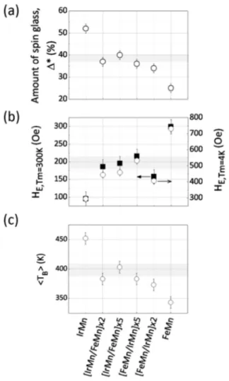
of blocking temperature distributions [32] and its extrapolation to 4K [21] offers a unique versatile way to quantify the glassy character of a FM/AFM interface. This was recently introduced by the SPINTEC laboratory [21] and thoroughly studied since then. In particular, by tuning various parameters such as the AF material (IrMn vs FeMn and NiMn) [21], F/AF interfacial mixing [35] via thermally activated species diffusions [36], the AF crystallography (polycrystalline- vs epitaxial-AF) [37] and lateral sizes [38], some of the key parameters influencing the formation of these F/AF spin-glass phases were identified and especially the role of Mn diffusions for Mn-based AF. Later on in this manuscript, we will deeply study the effect of Mn-diffusion, solutions to avoid such diffusion and the insights that this quantitative approach brought for applied spintronics and in particular for thermally activated TA-MRAMs.

Finally by comparing the various amplitudes (∆) either between high- and low-T contributions to DTB for a given sample, or between low-T contributions for various samples

we can quantify the relative impact of the F/AF glassy character. Basically, the smaller the ∆, the less the amount of spin-glass like phases. We will use this later on. Prior to that, let us detail some of the applications using exchange bias. Next, I will briefly introduce the notions of giant and tunnel magnetoresistance, the sensors applications and I will extensively describe memories applications and in particular thermally-assisted (TA) magnetic random access memories (MRAM). Essentially, this PhD work was done in the context of TA-MRAM. At the end of the next section, the issues related to TA-MRAM and the problems tackled in the frame of this PhD will be introduced.

(33)

(34)

Chapter 2. Applications of exchange bias and

issues to be solved

Spintronics applications such as thermally assisted MRAM (TA-MRAM), sensors (e.g.. hard disk drive read head), logic devices and radiofrequency emitters use F/AF EB interactions to set the reference direction required for the spin of conduction electrons. In this chapter, I will briefly discuss the principles of giant and tunnel magnetoresistance, that of a spin-valve with exchange bias F/AF bilayers and the applications employing these phenomena. Among the numerous kinds of devices employing magnetic properties, from very precise medical tools and microscopes to hard machinery and transducers, there are two major domains which are closely related to the current study. One of them is developed to detect magnetic field and the other stores data. Thus, the former belongs to the sensors family and the latter to the memories. Both of these families experienced a significant improvement over the last decades, not only because of modern technological facilities, but also thanks to several breakthrough discoveries. Nevertheless, the evolution of any technology happens step by step. I will focus on the evolution of sensors employed in HDDs read heads since the discovery of giant magnetoresistance (GMR) in 1988, and of another type of solid-state non-volatile magnetic data storage technology: magnetic random access memories (MRAM), since most of the work done in this PhD relates to MRAM.

2.1. Introduction of key concepts

2.1.1. Giant magnetoresistance

The discovery and interpretation of the giant magnetoresistance (GMR) phenomenon was rewarded by the Nobel prize in 2007. In 1988, Pr Peter Grunberg [39] and Pr Albert Fert [40] independently discovered this phenomenon in (Fe/Cr) sandwiches and multilayers. Their groups studied multilayered magnetic structures consisting of alternation of magnetic

(35)

Chapter 2 Applications of exchange bias and issues to be solved

and non-magnetic layers. Repeated Fe/Cr(tCr) multilayers with varied Cr thickness (tCr) were

studied, i.e. Fe thin layers separated by non-magnetic Cr metallic spacers. The first experimental result is shown in Figure 2.1a) for various thicknesses of Cr interlayer.

Figure 2.1

a) R(H) loops measured at 4.2K for [Fe (3nm)/ Cr (tCr)]N multilayers with tCr equal to 1.8, 1.2 and 0.9 nm and N repetitions = 30,35 and 60 respectively (After [40]). b) Schematically illustrated GMR scheme for 2 different F-layers orientation. Up-left – parallel configuration with low-resistance and up-right with a high resistance states. Bottom, corresponding sketch with the simplified equivalent electric circuit indicating the total resistance of the device. After [41].

The working principle of this system is based on a specific electron property – its spin, or more precisely on the spin-dependent conductivity in magnetic transition metal. The electrical current can be considered as carried in parallel by the spin “up” and spin “down” electrons. The notion of up and down refers to the spin-orientation relatively to the local magnetization. The resistivity of spin up and spin down electrons are equal in non-magnetic materials such as Cu or Al. However, in magnetic transition metal such as Fe, Ni and Co, the resistivity becomes spin-dependent. This is due to the different density of states at the Fermi for “up” and “down” spins orientation. Accordingly, the phenomenon of GMR arises from the spin dependent scattering phenomenon occurring in the bulk of the magnetic layers and their intefaces with the non-magnetic spacer. The overall electron scattering rate depends on the relative orientation of the magnetization in the successive ferromagnetic layers. (see Figure 2.1b)). Thus the two oppositely oriented populations of electrons propagating from one magnetic material to another through the non-magnetic spacer behave differently. Let us consider a three layer structure with F-layers separated by a non-magnetic spacer. When the two F layers are in parallel magnetic configuration, the system is in the low resistance state Figure 2.1b). Indeed, in this case the population of electrons with spins parallel to the

(36)

magnetization direction can easily traverse all layers with weak scattering. These spin up electrons can then carry lot of current and create a sort of short-circuit in the system. The spin-down electrons are strongly scattered in both magnetic layers but still the resistance is low due to the short-circuit effect of the spin-up electrons. If now the system is switched in the antiparallel magnetic configuration, both populations are affected Figure 2.1c) in either of the two F-layers. Now both categories of electrons are strongly scattered in one or the other ferromagnetic layers. The short-circuit effect of spin-up electrons present in parallel magnetic configuration no longer exists in the antiparallel configuration. As a result, the resistance becomes higher. Underneath sketched paths of electrons for each configuration, there is an equivalent resistance circuit for both configurations (Figure 2.1b-c). In this manner, by varying the magnetization direction of one magnetic layer so as to change the magnetic configuration from parallel to antiparallel, it becomes possible to achieve two distinct resistance states of the system.

Following the above sketched equivalent resistance circuits, one can derive the total resistance of the system in parallel and antiparallel orientations and the GMR ratio:

TU _X2T↑↓X↑↑ ↑↑ T↓↑ ; T U T↑↓ X↑↑ 2 (2.1) Z T T U_T TU U T↑↓ X↑↑ 4T↑↓X↑↑ (2.2)

2.1.2. Tunnel magnetoresistance

In 1970 spin-polarized tunneling was predicted by Tedrow and Meservey [42] and experimentally reproduced by Julliere [43] 5 years after. Studying Fe/GeO/Co structures, he found a resistance variation depending on the mutual orientation of the F-layers magnetization. As predicted by Slonczewski [44], the conductance of magnetic tunnel junctions is expected to be proportional to the cosine of the angle between the magnetization of the two F layers. Hence, the highest conductance (i. e. lowest resistance) is observed in the collinear case. Nevertheless, the interest for magnetic tunnel junctions dramatically increased when it became possible to perform magnetic tunnelling experiments at room temperature [45,47] with as much as 12% of MR ratio Figure 2.2a). These results were obtained with amorphous Alumina barrier. In these MTJ, the TMR amplitude is only determined by the electron polarization at the Fermi energy in the ferromagnetic electrodes. This polarization is equal to the relative difference in density of states at Fermi energy for

(37)

spin up and spin down electrons in the ferromagnetic layers. Following this breakthrough discovery, many studies were dedicated to increasing the tunnel magnetoresistance (TMR) amplitude by a proper choice of the tunnel barrier material. One of the best candidates as insulating layer which was predicted in 2001 [48,49] is thin crystalline MgO 001 [50] layer. The major difference between MgO and Alumina barrier is that the former are crystalline with good crystal matching with the ferromagnetic electrodes whereas the latter are amorphous. Thanks to this crystallinity, a new spin-filtering mechanism takes place associated with the symmetry of the wave functions. Electrons with _∆1 symmetry can tunnel easily through MgO barriers. It turns out that only spin up electrons have this ∆ 1 symmetry in Fe so that spin up electrons can easily tunnel in parallel magnetic configuration but not in antiparallel magnetic configuration [51]. This additional spin-filtering mechanism allows to significantly increase the TMR amplitude. In the late 90s, with Alumina barrier, the observed TMR were in the range 40-70% at room-temperature.[52–55].In 2004, TMR over 200% at RT were reported with MgO based crystalline MTJ, 410% TMR in 2006 [56] in 2007 500% [57] TMR was reached. In the following two subchapters, 2 different families of applications based on the above described phenomena will be discussed.

Figure 2.2

a) Room-Temperature magnetoresistance (R-H) loops for CoFe/Al2O3/Co tunnel junction. After [45]. b) Parallel and c) antiparallel F-layers mutual magnetization orientation with corresponding spins’ densities of d-states. After [46].

Tunneling Magneto Resistance (TMR) schematically is very similar to the GMR concept, apart from its physical origin due to the nature of material that separates F layers. Rather than using NM conducting layer like in GMR, for the TMR an insulator is inserted between magnetic electrodes. Applying voltage to F-electrodes and having thin enough insulator, there is a quantum mechanical probability for electrons to tunnel through the insulating layer. The TMR can be written as follows:

(38)

C T T U_T TU

U

2F(F

1 F(F (2.3)

where Pi is the polarization of the density of states (DOS) at the Fermi level for each F

layer surrounding the tunnel barrier:

F[ R_R[↑ \ R[↓ \

[↑ \ R[↓ \ (2.4)

2.1.3. Spin-valve

The spin-valve concept proposed in 1991 [58] consists in pinning the magnetization direction of one of the F-layers (in this case, the reference layer) by coupling this layer to an additional adjacent AF layer to pin it . Thanks to the F/AF exchange coupling, the F layer magnetization becomes stable and acts as a reference, while the magnetization of the sense F-electrode is free and therefore can easily rotate towards the applied field direction. The corresponding R-H loop on Figure 2.3b) shows the magnetic and transport responses of this system. Contrary to the first GMR-sandwiches consisted of two F-layers (Fe) coupled antiferromagnetically through a NM (Cr) spacer, spin-valve concept consists of two uncoupled F-layers separated by a non-magnetic spacer layer inducing no or only very weak interlayer coupling (typically Cu more than 2nm thick). Following this concept, the sensitive free layer magnetization is able to detect low fields while the pinned layer magnetization remains in a fixed direction reference. Spin-valves thus provided extremely sensitive magnetic field sensors and have been used as read head in hard disk drives between 1997 and 2004. (For detailed spin-valve review see for example - [59]).

(39)

Figure 2.3

(a) hysteresis loop and (b) magnetoresistance loop at room-T and (c) magnetoresistance loop at 78K;for a sample with composition: Si/ NiFe (15nm)/ Cu (2.6nm)/ NiFe (15nm)/ FeMn (10nm)/ Ag (2nm). The field is cycled along the FeMn FC direction. After [60].

2.2. Magnetoresistive read heads for hard disk drives

Many devices such as cell phones, smart-phones but also automotive or robotics require position and orientation sensors. When IBM introduced the AMR read-heads, replacing inductive coils it was already a giant leap in magnetic storage industry and led to a period of rapid areal density increase up to 1Gb HDD capacity with the rate about 60%/year for the areal density increase. The following years researchers were looking for a solution to further improve the scalability. With the AMR-based devices the main difficulty was related with the origin of phenomenon. Being a bulk effect, to be able to detect change in magnetization coming from tiny area, the sensor itself should be comparably small. With AMR, lowering the thickness lowers the output signal strength. This comes from the electrons property – with the film thickness up to couple of tens nanometers they start scattering out of the film surface up to an extent when signal to noise ratio becomes crucial. Therefore AMR-based read-heads could not be considered as a promising technology to increase areal density for the recording media. Being an interfacial effect, GMR was the best candidate to replace previous technology, with its high output signal at very low thickness of sense layer.

(40)

Figure 2.4

The evolution of magnetic storage industry: a) IBM 350 model with 5 Mb capacity introduced in 1956 [61] (picture from [62]), b) Micro SD card with 64 Gb storage capacity on a human finger (picture from [63]), and c) time evolution of the data storage areal density, after [64].

Having just a few percent of MR ratio for AMR and a couple of tens percent for GMR, one can guess how rapidly the further progress was evolving. To have a basic idea on how revolutionary it impacted magnetic recording industry, two numbers will make this impression. Before the introduction of GMR-based magnetic read-heads in 1997 the areal density was only 1 Gbit/in2 whereas 10 years later IBM showed a hard drive with the value of 300Gbit/in2. This huge technological leap completely changed recording media market. The famous Moore’s law reflecting the evolution of the number of transistors with the time has an analogy, representing the memory areal density reduction (Figure 2.4) for so-called magnetic areal density. This parameters simply tell us how small in its lateral dimensions can be written a Boolean elements – logic “1” or “0”. This correspondence becomes natural if one considers the more and more powerful machines and computers that obviously lead to the development of related technological progress in various areas. The quality of digital cameras, videos, photos, internet solutions and other media, demands larger storage capabilities.

Even though it may seem easy to implement new GMR-based approach, having good MR ratio, in a fully functional device, in fact there were a lot of efforts done to bring it to the market, especially dealing with low scales. One of the difficulties in GMR-based device implementation was related with magnetic field to reverse the magnetization of the storage layer. Being coupled antiferromagnetically (otherwise the system will be always in parallel state), the applied field to reverse the magnetization of storage layer should be strong

(41)

enough to overcome the AF coupling energy. Although, showing high MR ratio at low temperatures, the MR amplitude decreases significantly with temperatures and was requiring high field to be obtained (the MR about 65% at RT for Co/Cu multilayers was reached in 1991 [65] and required saturation field as big as 10kOe, whereas 35% of MR were available at only 300 Oe). Furthermore, in order to reduce the lateral dimensions of one bit - the read-head size had to be reduced accordingly, leading the storage and reference to become thinner and thinner. This issue was solved thanks to the spin-valve concept presented previously [59].

Figure 2.5

Picture of real HDD drive (left) with a sketch of the read-head (up-right). The Reference and free layer’s easy axes are perpendicular. Below the spin-valve structure is also sketched the track of “0” and “1” bits.

As it is schematically illustrated on Figure 2.5, the read-head flying above the surface of the disc senses the magnetic field coming from the underneath media. Obviously, the thickness of the free layer should not be greater than the length of each bit in the downtrack direction, otherwise the signal from two neighbouring bits would be detected, that in turn will lead to high error rate and big signal to noise ratio. In terms of media, a significant improvement has been the change from in-plane to out-of-plane magnetized media. Before, the magnetization was in plane and the bit readout was based on domain boundaries detection, producing stray fields. With the time, it became obvious, that longitudinal magnetization approach was reaching its limit with bit size reduction. The reason was that data retention for 10 years imposes the requirement KeffV > 67 kBT. where KeffV – anisotropy

energy, Keff – anisotropy constant, V –the volume of the grain, kB – Boltzmann constant. Keff,

being a fixed parameter as a material property, with continuous decrease of bit size (volume V accordingly), would lead to super-paramagnetic limit. The out-of-plane magnetic recording approach was proposed to push further the density of bits per unit area. Indeed, when the magnetization points out-of-plane, the demagnetizing field decreases while reducing the bit

(42)

size. This magnetic configuration allowed increasing the areal density up to 750 Gbits/in2, which is 18 times denser than for longitudinal media. In 2005 Seagate Corporation launched HDDs with heads based on TMR effect. Their larger MR ratios allowed keeping on increasing the storage capabilities of HDDs. High TMR ratios provide high signal to noise ratio provided the resistance area (RA) product can be maintained sufficiently low so that the sensor resistance remains in the range of a few tens of ohm and keep the shot noise low enough. [66].

2.3. Memories

Another family of devices based on the TMR-effect is magnetic random access memories (MRAM). In contrast to sensors where the magnetization of the free layer coherently rotates around a 90° orientation with the magnetization of the reference layer, in memory, the magnetization of the soft layer (called storage layer), can lie in two possible stable states (parallel or antiparallel magnetic configurations) with two associated values of MTJ resistance. The magnetization direction is switched either by application of a magnetic field or by using the spin-transfer-torque phenomenon. The information is stored as the magnetic orientation of the storage layer magnetization. The readout is achieved by measuring the resistance of the stack. In terms of fabrication, memories are much more demanding in terms of process control than read-heads. Indeed, read heads comprise only one MTJ and can be tested and selected one by one. In contrast, memories comprise millions or even billions of MTJs which must have very similar properties. The larger the memory capacity, the more stringent the constrains on the process quality.

From the very beginning, the MRAM concept attracted a worldwide attention that can be easily explained. MRAM have lot of advantages compared to other memory technologies: i) As FLASH memories and in contrast to DRAM or SRAM, they are non-volatile (no loss of data when the power is off); ii) they can be as dense as DRAM iii) Their data retention can exceed 10 years; iv) They have almost infinite endurance meaning that they can be written more than 1016 cycles which is much better than all other technologies of non-volatile memories (FLASH: endurance~105cycles) v) They can be written and read with low power consumption and vi) at high read/write speed (write speed ~3-10ns; read speed~10ns). These memories are solid state memories meaning that in contrast to HDD, the stored information can be accessed without any mechanical movement and in random order (random access memories)

Over the two last decades, many MRAM concepts were proposed for various types of applications. They will be discussed in the next section.

Ferromagnetic/antiferromagnetic exchange bias nanostructures for ultimate spintronic devices

HAL Id: tel-01161786

https://tel.archives-ouvertes.fr/tel-01161786

Ferromagnetic/antiferromagnetic exchange bias

nanostructures for ultimate spintronic devices

Kamil Akmaldinov

To cite this version:

THÈSE

DOCTEUR DE L’UNIVERSITÉ DE GRENOBLE

Kamil AKMALDINOV

Ferromagnetic/antiferromagnetic

exchange bias nanostructures

for ultimate spintronic devices

Contents

INTRODUCTION

Chapter 1.

Introduction to ferromagnetic /

antiferromagnetic exchange bias

1.1.

Exchange bias phenomenology

1.1.1.

Discovery

1.1.2.

Setting exchange bias

1.2.

Theoretical models

1.2.1.

Meikeljohn and Bean intuitive picture

1.2.2.

Néel/Mauri domain wall model

1.2.3.

Magnetic frustrations: Malozemoff’s random field and Takano models

1.2.4.

Todays’ macroscopic picture:

granular model plus spin-glass like phases

1.3.

Quantifying the amount of spin-glass like phases

Chapter 2.

Applications of exchange bias and

issues to be solved

2.1.

Introduction of key concepts

2.1.1.

Giant magnetoresistance

2.1.2.

Tunnel magnetoresistance

2.1.3.

Spin-valve

2.2.

Magnetoresistive read heads for hard disk drives

2.3.

Memories