HAL Id: inria-00321766
https://hal.inria.fr/inria-00321766
Submitted on 15 Sep 2008
HAL is a multi-disciplinary open access
archive for the deposit and dissemination of
sci-L’archive ouverte pluridisciplinaire HAL, est
destinée au dépôt et à la diffusion de documents
Functions
Pascal Berthomé, Nicolas Nisse
To cite this version:
Pascal Berthomé, Nicolas Nisse. A unified FPT Algorithm for Width of Partition Functions. [Research
Report] RR-6646, INRIA. 2008, pp.36. �inria-00321766�
a p p o r t
d e r e c h e r c h e
-6 3 9 9 IS R N IN R IA /R R --6 6 4 6 --F R + E N G Thème COMA unified FPT Algorithm for Width of Partition
Functions
Pascal Berthomé — Nicolas Nisse
N° 6646
Functions
Pascal Berthom´e
∗, Nicolas Nisse
†Th`eme COM — Syst`emes communicants Projets Mascotte
Rapport de recherche n°6646 — September 2008 — 36 pages
Abstract: During the last decades, several polynomial-time algorithms have been designed that decide if a graph has treewidth (resp., pathwidth, branchwidth, etc.) at most k, where k is a fixed parameter. Amini et al. (to appear in SIAM J. Discrete Maths.) use the notions of partitioning-trees and partition functions as a generalized view of classical decompositions of graphs, namely tree-decomposition, path-decomposition, branch-decomposition, etc. In this paper, we propose a set of simple sufficient conditions on a partition function Φ, that ensures the existence of a linear-time explicit algorithm deciding if a set A has Φ-width at most k (k fixed). In particular, the algorithm we propose unifies the existing algorithms for treewidth, pathwidth, linearwidth, branchwidth, carvingwidth and cutwidth. It also provides the first Fixed Parameter Tractable linear-time algorithm deciding if the q-branched treewidth, defined by Fomin et al. (Algorithmica 2007), of a graph is at most k (k and q are fixed). Our decision algorithm can be turned into a constructive one by following the ideas of Bodlaender and Kloks (J. of Alg. 1996).
Key-words: Tree-decomposition, FPT-algorithm, width-parameters, characteristics.
This work was partially funded by the support of CONICYT via Anillo en Redes ACT08, and of the European projects 1ST FET AEOLUS and COST 293 GRAAL.
∗LIFO, ENSI-Bourges, Universit´e d’Orl´eans, Bourges, France.{[email protected]@sophia.inria.fr †MASCOTTE, INRIA, I3S, CNRS, UNS, Sophia Antipolis, France. {[email protected]
partition
R´esum´e : Depuis une vingtaine d’annes, de nombreux algorithmes polynomiaux ont ´et´e con¸cu pour les probl`emes consistant `a d´ecider si la largeur arborescente (resp., largeur lin´eaire, largeur en branche, etc.) d’un graphe est au plus k, o`u k est un param`etre fix´e. Amini et al. (`a paraˆıtre dans SIAM J. Discrete Maths.) utilisent les notions d’arbre de partition et de fonctions de partition pour g´en´eraliser les d´ecompositions “classiques” des graphes, comme par exemple la d´ecomposition arborescente, la d´ecomposition lin´eaire, la d´ecomposition en branches, etc. Dans ce papier, nous proposons des conditions simples et suffisantes qui, si elles sont satisfaites par une fonction de partition Φ, suffisent `a assurer l’existence d’un algorithme lin´eaire qui d´ecide si un ensemble A poss`ede une Φ-largeur au plus k (k ´etant fix´e). En particulier, l’algorithme que nous proposons unifie les algorithmes existants pour la largeur arborescente, la largeur lin´eaire, la largeur en branche, etc. Notre algorithme est ´egalement le premier algorithme FPT d´ecidant en temps lin´eaire si la largeur arborescente q-branch´ee, d´efinie par Fomin et al. (`a paraˆıtre dans Algorithmica), d’un graphe est au plus k (k et q ´etant fix´es). Notre algorithme de d´ecision peut ˆetre modifi´e en un algorithme constructif en utilisant les id´ees de Bodlaender and Kloks (J. of Alg. 1996). Mots-cl´es : D´ecomposition arborescente, algorithme FPT, largeurs de graphes, car-act´eristique.
1
Introduction
The notion of treewidth is central in the theory of the Graph Minors developed by Robertson and Seymour [RS86]. Roughly, the treewidth of a graph measures how close a graph is to a tree. More formally, a tree-decomposition (T, X ) of a graph G = (V, E) is a tree T together with a family X = (Xt)t∈V(T ) of subsets of V , such that: (1) St∈V(T )Xt= V , (2) for any
edge e = {u, v} ∈ E, there is t ∈ V (T ) such that u, v ∈ Xt, and (3) for any v ∈ V , the set
of t such that v ∈ Xtinduces a subtree of T . The width of (T, X ) is the maximum size of
Xtminus 1, t ∈ V (T ), and the treewidth tw(G) of a graph G is the minimum width among
its tree-decompositions. If T is restricted to be a path, we get a path-decomposition of G, and the pathwidth pw(G) of G is the minimum width among its path-decompositions.
Both pathwidth and treewidth have a nice theoretical-game interpretation (see [Bie91, FT08] for surveys). Pathwidth can be described as a graph searching game where a team of searchers aims at capturing an invisible and arbitrary fast fugitive hidden on the vertices of the graph, whereas treewidth deals with the capture of a visible fugitive. In [FFN07], Fomin et al. introduce a variant of these games, called non-deterministic graph searching, that establishes a link between pathwidth and treewidth. Loosely speaking, in non-deterministic graph searching, the fugitive is invisible, but the searchers are allowed to query an oracle that possesses complete information about the position of the fugitive. However, the number of times the searchers can query the oracle is limited. The q-limited search number of a graph G, denoted by sq(G), is the smallest number of searchers required to capture an invisible
fugitive in G, performing at most q ≥ 0 queries to the oracle. Fomin et al. give the following interpretation of non-deterministic graph searching in terms of graph decomposition. A tree-decomposition (T, X ) is q-branched if T can be rooted in such a way that any path from the root to a leaf contains at most q ≥ 0 vertices with at least two children. q ≥ 0 being fixed, the q-branched treewidth twq(G) of a graph G is the minimum width among its
q-branched tree-decompositions (tw∞(G) = tw(G) and tw0(G) = pw(G)). For any q ≥ 0 and
any graph G, sq(G) = twq(G) + 1 [FFN07, MN08]. Fomin et al. prove that deciding sq(G) is
NP-complete for any q ≥ 0, and design an algorithm that decides whether sq(G) ≤ k in time
O(nk+1) for any n-node graph G [FFN07]. Prior to this work, no explicit Fixed Parameter
Tractable (FPT) algorithm for this problem was known.
The notion of treewidth also plays an important role in the domain of algorithmic com-putational complexity. Indeed, many graph theoretical problems that are NP-complete in general are tractable when input graphs have bounded treewidth. Thus, an impor-tant challenge consists in computing optimal tree-decompositions of graphs. Much re-search has been done on the problem of finding an optimal tree-decomposition. This prob-lem is NP-complete [ACP87] and special interest has been directed toward special graph classes [Bod93, BM93, BKK95]. The case of the class of graphs with bounded treewidth has been widely studied in the literature [ACP87, Ree92].
In their seminal work on Graph Minors [RS94, RS04], Robertson and Seymour give a non-constructive proof of the existence of a O(n2) decision algorithm for the problems of
k, the class of graphs of treewidth at most k is minor-closed, an immediate consequence is the existence of a polynomial-time algorithm deciding whether a graph has treewidth at most k, where k is a fixed parameter. In [BK96], Bodlaender and Kloks design a linear time algorithm for solving this problem. More precisely, k and k′ being fixed, given a n-node graph G and a
tree-decomposition of width at most k′ of G, the Bodlaender and Kloks’ algorithm decides
if tw(G) ≤ k in time O(n). The big-oh hides a constant more than exponential in k and k′.
In the last decades, analogous algorithms have been designed for other width parameters of graphs like pathwidth [BK96], branchwidth [BT97], linearwidth [BT04], carvingwidth and cutwidth [TSB00]. These algorithms are mainly based on the notion of characteristic (see Section 4). This paper aims at unifying and generalizing these FPT algorithms. As a particular application, our algorithm decides in linear time if the q-limited search number of a graph G is at most k, q ≥ 0 and k ≥ 1 fixed.
In order to generalize the algorithm of [BK96], we use the notions of partition function and partitioning-tree defined in [AMNT07]. Given a finite set A, a partition function Φ is a function from the set of partitions of A into the integers. A partitioning-tree of A is a tree T together with a one-to-one mapping between A and the leaves of T . The Φ-width of T is the maximum Φ(P), for any partition P of A defined by the internal vertices of T , and the Φ-width of A is the minimum Φ-width of its partitioning-trees. Partition functions are a unified view for a large class of width parameters like treewidth, pathwidth, branchwidth, etc. In [AMNT07] is given a simple sufficient property that a partition function over A must satisfy to ensure that either A admits a partitioning-tree of width at most k ≥ 1, or there exists a k-bramble (a dual structure).
In this paper, we extend the definition of Φ-width to the one of q-branched Φ-width of a set A. Then, we use the framework of [BK96] applied to the notions of partition functions and partitioning-tree in order to design a unified linear-time algorithm that decides if a finite set has q-branched Φ-width at most k. Again, q ≥ 0 and k ≥ 1 are fixed parameters. Our results: We propose a simple set of sufficient properties and an algorithm such that, for any k and q fixed parameters, and any partition function Φ satisfying the properties, our algorithm decides in time O(|A|) if a finite set A has q-branched Φ-width at most k (Theo-rem 1). Since treewidth, pathwidth, branchwidth, cutwidth, linearwidth, and carvingwidth can be defined in terms of Φ-width for some particular partition functions Φ that satisfy our properties (Theorem 2), our algorithm unifies the works in [BK96, BT97, TSB00, BT04]. Moreover, our algorithm generalizes the previous algorithms since it is not restricted to width-parameters of graphs but works as well for any partition function (not restricted to graphs) satisfying some simple properties. Finally, it provides the first explicit linear-time algorithm that decides if a graph G can be searched in a non-deterministic way by k searchers performing at most q queries, for any k ≥ 1, q ≥ 0 fixed. Due to lack of space, most of the proofs are omitted and can be found in the Appendices.
2
Main theorem.
2.1
Partition function and partitioning-tree.
Let A be a finite set. Let P = {A1, · · · , Ar} and Q = {B1, · · · , Bp} be two partitions of A.
For any subset A′⊆ A, the restriction P ∩A′of P to A′is the partition {A
1∩A′, · · · , Ar∩A′}
of A′ (where the empty parts have been removed). Q is a subdivision of P if, for any j ≤ p,
there exists i ≤ r with Bj⊆ Ai.
A partition function ΦA over A is a function from the set of partitions of A into the
integers. ΦA is monotone if, for any subdivision Q of a partition P of A, ΦA(P) ≤ ΦA(Q).
A (monotone) partition function Φ is a function that associates a (monotone) partition function ΦAover A to any finite set A. A partition function Φ is closed under taking subset
if, for any A′⊆ A and any partition P of A, Φ
A′(P ∩ A′) ≤ ΦA(P).
A partitioning-tree (T, σ) of A is a tree T together with a one-to-one mapping σ between A and the leaves of T . If T is rooted in r ∈ V (T ), the partitioning-tree is denoted by (T, r, σ). Any internal vertex v ∈ V (T ) corresponds to a partition Tvof A, defined by the sets of leaves
of the connected components of T \ v. Similarly, any edge e ∈ E(T ) defines a bi-partition Teof A. The ΦA-width of (T, σ) is the maximum of ΦA(Tv) over the internal (i.e., non leaf)
vertices v of T . The Φ-width of A is the minimum ΦA-width of its partitioning-trees (cf.
Figure 1 in Appendix A).
A branching node of a rooted tree (T, r) is either the root or a vertex of T with at least two children. A tree T is q-branched if there exists a root r ∈ V (T ) such that any path from r to a leaf contains at most q ≥ 0 branching nodes. For instance, T is 0-branched if and only if T is a path. The corpse cp(T ) of a tree T denotes the rooted tree obtained from T by removing all its leaves. A partitioning tree (T, σ) is q-branched if the corpse cp(T ) of T is q-branched. For instance, a partitioning-tree (T, σ) is 0-branched if and only if T is a caterpillar. The q-branched Φ-width of A is the minimum ΦA-width of its q-branched
partitioning-trees.
2.2
Sufficient conditions for a linear time algorithm.
A nice decomposition (D, X ) of a finite set A is a O(|A|)-node rooted tree D, together with a familly X = (Xt)t∈V(D) of subsets of A such that, ∪t∈V(D)Xt= A, and for any v ∈ V (D):
(a) start node: v is a leaf, or (b) introduce-node: v has a unique child u, Xu ⊂ Xv and
|Xv| = |Xu| + 1, or (c) forget-node: v has a unique child u, Xv ⊂ Xu and |Xu| = |Xv| + 1,
or (d) join-node: v has exactly 2 children u and w, and Xv= Xu= Xw.
For any v ∈ V (D), let Dv denote the subtree of D rooted in v, and Av= ∪t∈V(Dv)Xt.
Let Φ be a partition function. A nice decomposition (D, X ) for A is compatible with Φ if
it exists a function FΦthat associates an integer FΦ(x, P, e) to any integer x, partition
P of some subset of A and element e of A, such that, F is strictly increasing in its first coordinate, and, for any introduce node v ∈ V (D) with child u, any partition P of Av,
it exists a function HΦ that associates an integer HΦ(x, y, P) to any pair of integers
x, y, and partition P of some subset of A, such that, F is strictly increasing in its first and second coordinates, and, for any join node v ∈ V (D) with children u and w, any partition P of Av,
ΦAv(P) = HΦ(ΦAu(P ∩ Au), ΦAw(P ∩ Aw), P ∩ Xv).
Intuitively, the existence of FΦand HΦmeans that it is possible to compute the Φ-width
of some partitions P without knowing explicitly P, but only knowing a restriction of P and the Φ-width of some restrictions of P, these restriction being defined by the decomposition (D, X ).
Theorem 1. Let Φ be a monotone partition function that is closed under taking subgraph. Let k, k′ ≥ 1 and q ≥ 0 be three fixed integers (q may be ∞). There exists an algorithm that
solves the following problem in time linear in the size of the input set:
input: a finite set A, and a nice decomposition (D, X ) for A that is compatible with Φ, and maxt∈V(D)|Xt| ≤ k′, output: decide if the q-branched Φ-width of A is at most k.
Guideline of the algorithm.
In the following, we define the notion of characteristic, Char((T, r, σ), X), of a partitioning-tree (T, r, σ) of A restricted to X ⊆ A (Section 4). Roughly, characteristics are a compact data structure encoding the information necessary to build partitioning-trees. Following the framework in [BK96], we prove that the number of characteristics of q-branched partitioning-trees with Φ-width at most k, restricted to X, is bounded by a function of q, k and |X| (this function does not depend on q when q = ∞). Then, we prove that the size of such charac-teristics is also bounded (Lemma 6). Finally, we define an ordering ¹ on the characcharac-teristics that allows us to consider only some specific characteristics. More precisely, given v ∈ V (D), a set of characteristics Set(v) is a set of characteristics of q-branched partitioning-trees of Av with Φ-width at most k, restricted to Xv. This set is said full if, roughly, all minimal
such characteristics belong to it (see Section 4). By definition, there is a non empty full set of characteristics F ullSet(v) if and only if the q-branched Φ-width of Av is at most k.
The algorithm proceeds by performing a dynamic programming. First, it computes a full set of characteristics F ullSet(v) for any start node (i.e., leaf) v ∈ V (D). Then, for any v ∈ V (D), a full set of characteristics F ullSet(v) is computed in constant time, starting from the full sets of characteristics of the children of v. This is the role of Procedures IntroduceN ode (Section 5.1.2), F orgetN ode (Section 5.2) and JoinN ode (Section 5.3). Therefore, in time |V (D)| = O(|A|), our algorithm computes a full set of characteristics F ullSet(rD) of the root of D. Since ArD = A, the q-branched Φ-width of Av is at most k
if and only if F ullSet(rD) 6= ∅.
In Sections 4 and 5, we present the main tools used in the design of our algorithm. First, in the next section, we present an important application of this theorem to the graphs.
3
Tractability of width-parameters of graphs.
This section is devoted to present an application of Theorem 1 in terms of graph’s pa-rameters. We first recall the definition of some graph’s parameters, and establish their relationship with partition functions [AMNT07].
Let G = (V, E) be a connected graph. Let ∆ be the function that assigns, to any partition X = {E1, · · · , Er} of E, the set of the vertices of G that are incident to edges in Ei and Ej,
with i 6= j. Let δ be the partition function that assigns |∆(X )| to any partition X of E. Treewidth [RS86]: The treewidth of G is at most k ≥ 1 if and only if there is a partitioning-tree of E with δ-width at most k + 1. Indeed, let (T, σ) be a partitioning-partitioning-tree of E, then (cp(T ), (Xt)t∈V(cp(T ))), with Xt = ∆(Tt), is a tree-decomposition of G. Conversely, let
(T, X ) be a tree-decomposition of G with width at most k. Then, for any edge {x, y} ∈ E, let us choose an arbitrary bag Xt that contains both x and y, add a leaf f adjacent to
t in T , and let σ(f ) = {x, y}. Finally, let S be the minimal subtree spanning all such leaves. The resulting tree (S, σ) is a partitioning-tree of E with δ-width at most k + 1 and T = cp(S) [AMNT07].
Pathwidth [RS83]: The pathwidth of G is at most k ≥ 1 if and only if there is a partitioning-tree (T, σ) of E with δ-width at most k + 1 and such that (T, σ) is 0-branched. q-branched treewidth [FFN07]: More generally, the q-branched treewidth of G is at most k ≥ 1 if and only if there is a q-branched partitioning-tree (T, σ) of E with δ-width at most k + 1. Recall that a partitioning-tree (T, σ) is q-branched if cp(T ) is q-branched.
Other partition functions defining branchwidth (br), linearwidth (lw), carvingwidth (carw), and cutwidth (cw) are described in Appendix F. The remaining part of this section is devoted to prove the Theorem 2 that is an important interpretation of Theorem 1 when width-parameters of graphs are concerned. We first need some lemmata. The following lemma is straightforward and its proof is thus omitted.
Lemma 1. Aforementioned partition functions are monotone and closed under taking sub-set.
Lemma 2. Let G be a graph with maximum degree deg. Given a nice tree-decomposition (T, Y) of G with width at most k′ ≥ 1, a nice decomposition (D, X ) of E, compatible with
the partition functions corresponding to treewidth (resp., branchwidth), q ≥ 0, and with maxt∈V(D)|Xt| ≤ k′· deg can be computed in linear time.
Proof. Due to lack of space, we only prove the lemma for the partition function corresponding to treewidth. First, it is easy to obtain a nice decomposition (D, X ) of E from (T, Y). For any v ∈ V (T ), let Tv denote the subtree of T rooted in v, and Av= ∪t∈V(Tv)Yt, and let Ev
be the set of edges belonging to the subgraph induced by the vertices contained in Av that
are incident to a vertex in Yv. Any start node, resp., join node, Ytof (T, Y) corresponds to
a start node, resp., join node, Etof (D, X ). For any introduce node Yt of (T, Y), let x ∈ V
be the vertex such that Yt= Yt′∪ {x}, where t′ is the single child of t in T . Let e1, · · · , er
path of introduce nodes E(G[Yt′])∪{e1}, E(G[Yt′])∪{e1, e2}, · · · , E(G[Yt′])∪{e1, e2, · · · , er}
in (D, X ). Finally, any forget node Yt of (T, Y) is modified into a path of forget nodes
E(G[Yt′]) \ {e1}, E(G[Yt′]) \ {e1, e2}, · · · , E(G[Yt′]) \ {e1, e2, · · · , er} in (D, X ), where t′ is
the unique child of t in T , and e1, · · · , er are the edges that are incident to x = Yt′ \ Yt
and to no other vertex in Yt. The obtained decomposition of E is a nice decomposition
and its width (i.e., the maximum number of edges in each bag) is at most the width of the tree-decomposition (T, Y) times the maximum degree of G.
It remains to prove that (D, X ) is compatible with δ. Let Fδ be defined as follows.
Definition 1. Let x be an integer, P be a partition of a subset E′ of E and an edge e ∈ E′.
Then, Fδ(x, P, e) = x + |{v ∈ e | v ∈ ∆(P) \ ∆(P ∩ (E′\ {e}))}|.
That is, Fδ adds to x the number of vertices incident to e that contribute to the border
of the partition P because they are incident to e. Fδ is obviously strictly increasing in its
first coordinate. Moreover, it can be computed in constant time when |E′| is bounded by a
constant.
For any v ∈ V (D), let Dv denote the subtree of D rooted in v, and Av= ∪t∈V(Dv)Xt.
Let v ∈ V (D) be an introduce node with child u, and let {e} = Xv\ Xu. Let P be a
partition of Av. We need to prove that δAv(P) = Fδ(δAu(P ∩Au), P ∩Xv, e). In other words,
let us prove that δAv(P) = δAu(P ∩ Au) + |{v ∈ e | v ∈ ∆(P ∩ Xv) \ ∆(P ∩ Xv∩ (Xv\ {e}))}|.
δAv(P) is the number of vertices in the subgraph induced by the set of edges Av, that are
incident to edges in different parts of P. This set of vertices can be divided into two disjoint sets: (1) the set S1of vertices that are incident to two edges f and h that are different from
e and that belong to different parts of P, and (2) the set S2 of vertices x incident to e and
such that all other edges (different from e) incident to x belong to the same part of P that is not the part of e. S1 is exactly the set of vertices belonging to ∆Au(P ∩ Au), therefore
|S1| = δAu(P ∩ Au).
By definition of (D, X ) (because it has been built from a tree-decomposition), any edge of Au= Av\ {e} that has a common end with e belongs to Xv. Therefore, any vertex in S2
belongs to ∆(P ∩ Xv). It is easy to conclude that |S2| = |{v ∈ e | v ∈ ∆(P ∩ Xv) \ ∆(P ∩
Xv∩ (Xv\ {e}))}|.
Therefore, the function Fδ satisfies the desired properties. Let Hδ be defined as follows.
Definition 2. Let x and y be two integers, and let P be a partition of a subset E′ of E.
Then, Hδ(x, y, P) = x + y − δ(P).
Hδ is obviously strictly increasing in its first and second coordinates. Moreover, it can
be computed in constant time when |E′| is bounded by a constant.
Let v ∈ V (D) be a join node with children u and w, and let P be a partition of Av, we
must prove that δAv(P) = Hδ(δAu(P ∩ Au), δAw(P ∩ Aw), P ∩ Xv). That is, we prove that
δAv(P) = δAu(P ∩ Au) + δAw(P ∩ Aw) − δXv(P ∩ Xv).
First, note that ∆Au(P ∩ Au) ∪ ∆Aw(P ∩ Aw) ⊆ ∆Av(P). Moreover, by definition of the
Indeed, Xv has been built by taking all edges incident to a vertex in a bag Y of the
tree-decomposition (T, Y). By the connectivity property of a tree-tree-decomposition, if a vertex x would have been incident to an edge in Au\ Aw and to an edge in Aw\ Au, then x ∈ Y
which would have implied that both these edges belong to Xv = Au∩ Aw, a contradiction.
Therefore, ∆Av(P) ⊆ ∆Au(P ∩ Au) ∪ ∆Aw(P ∩ Aw). To conclude, it is sufficient to observe
that ∆Au(P ∩ Au) ∩ ∆Aw(P ∩ Aw) = ∆Xv(P ∩ Xv).
Due to lack of space the proof of the following lemma is omitted and can be found in Appendix F.2.
Lemma 3. Any nice tree-decomposition (T, Y) of G is a nice decomposition of V that is compatible with the partition functions corresponding to carwingwidth (resp., cutwidth).
Bodlaender designs a linear-time algorithm that decides if the treewidth of a graph G is at most k, and, if tw(G) ≤ k returns a tree-decomposition of width at most O(k) [Bod96]. Moreover, a nice decomposition of G can be computed in linear time from any tree-decomposition of G, and without increasing its width [BK96]. Finally, for any graph G and any q ≥ 0, tw(G) ≤ twq(G) ≤ pw(G) (By definition), tw(G) ≤ 32bw(G) [RS91], pw(G) ≤
cw(G) [TSB00], tw(G) ≤ 3carw(G) [TSB00] and pw(G) ≤ lw(G) [BT04]. Therefore, as an application of Theorem 1, Lemmata 1,2 and 3 lead to:
Theorem 2. Let k and q be two fixed parameters. There exists an algorithm that solves the following problem in time linear in the size of the input.
input: A graph G with degree bounded as a function of q and k, output: Decide if G has q-branched treewidth, resp., branchwidth, linearwidth, carvingwidth or cutwidth at most k.
4
Characteristics of partitioning-trees.
This section is devoted to define the characteristic of any rooted partitioning-tree of some finite set A when we “restrict” it to a subset B ⊆ A. Let Φ be a monotone partition function.
4.1
Contraction of labeled path
One of the main tool that we use is the contraction of labeled paths. A labeled path is a path the vertices and edges of which are labeled by integers. In the following, any path of a partitioning tree of A will be considered as a labeled path, the vertices and edges being labeled by the ΦA-width of the partition they correspond to. Note that, because Φ is
monotone, the label of any edge is at most the minimum label of its ends.
Let P = {v0, v1, · · · , vn} be a path where any vertex vi is labeled with an integer ℓ(vi),
and any edge ei= {vi−1, vi} with an integer ℓ(ei). To define the contraction of P , we revisit
the notion of typical sequence of a sequence of integers [BK96] (see Appendix B.1). Roughly, the goal of the following operation is to contract some edges and vertices of P that are not “necessary” to remember the variations of the sequence (ℓ(v0), ℓ(e1), ℓ(v1), · · · , ℓ(en), ℓ(vn)).
The contraction Contr(P ) is the path obtained from P , with same ends, by contracting some edges and vertices obtained by the following procedure. Start with one integral variable m = 1. While m 6= n, do the following. Let i, m ≤ i ≤ n − 1, be the greatest index such that, for any m ≤ j ≤ i, ℓ(em) ≤ ℓ(ej)) ≤ ℓ(vi) and ℓ(em) ≤ ℓ(vj)) ≤ ℓ(vi). Contract all
vertices and edges between e and vi. Then, set m to the greatest index such that, for any
i < j ≤ m, ℓ(vi) ≥ ℓ(ej) ≥ ℓ(em) and ℓ(vi) ≥ ℓ(vj) ≥ ℓ(em). Contract all vertices and edges
between vi and em. Edges and vertices of Contr(P ) keep their initial label (cf. Figure 2 in
Appendix A).
The crucial property of Contr(P ) = {v0= v′0, v1′, · · · , vp−1′ , vp′ = vn} is that the sequence
S′ = (ℓ(e′
1), ℓ(v1′), · · · , ℓ(e′p−1), ℓ(vp−1′ ), ℓ(e′p)) (where e′i = {vi−1′ , vi′}) is “almost” the
typi-cal sequence of the sequence S = (ℓ(e1), ℓ(v1), · · · , ℓ(en)). More precisely, if ℓ(e′1) 6= ℓ(v1′),
then S′ = τ (S), otherwise (ℓ(v′
1), ℓ(e′2), · · · , ℓ(vp−1′ ), ℓ(e′p)) = τ (S) (τ (S) denotes the
typ-ical sequence of S). Moreover, it is important to note that any v ∈ V (Contr(P )) (e ∈ E(Contr(P ))) represents a unique v∗∈ V (P ) (e∗∈ E(P )).
We define max(P ) as the maximum integer labeling an edge or a vertex of a labeled path P . Similarly, we define min(P ). The following lemma is straightforward when using the fact that the number of different typical sequences of integers in {0, 1, · · · , k} is at most
8
32
2k [BK96].
Lemma 4. Let P be a labeled path.
1. min(Contr(P )) = min(P ) and max(Contr(P )) = max(P ).
2. The number of contractions of paths P with max(P ) ≤ k is bounded by a function of k. In the following, we need to order the labeled paths. An extension of a labeled path P is any path obtained by subdividing some edges of P an arbitrary number of times. Both edges and the vertex resulting from the subdivision of an edge e are labeled with ℓ(e). Given two labeled paths P and Q, we say that P ¹ Q if there is an extension P∗ = {p
1, · · · , pr}
of P and an extension Q∗= {q
1, · · · , qr} of Q with same length, and such that ℓ(pi) ≤ ℓ(qi)
and ℓ({pi, pi+1}) ≤ ℓ({qi, qi+1}) for any i ≤ r.
4.2
Restriction of a partitioning-tree
Let (T, r, σ) be a partitioning-tree of A. Any internal vertex v ∈ V (T ) is labeled by ℓ(v) = ΦA(Tv) and any edge e ∈ E(T ) is labeled by ℓ(e) = ΦA(Te). To avoid technicality, we
assume that T is not restricted to an edge, and r is not a leaf of T . Therefore, the corpse cp(T ) (T without its leaves) can be rooted in r. The restriction Char((T, r, σ), B) of (T, r, σ) to B is a rooted partitioning-tree (T∗, r∗, σ∗) of B, together with a labeling function ℓ∗ :
V (cp(T∗)) ∪ E(T∗) → N, an integer dist∗, a subset K∗ of vertices of T∗ such that any
v ∈ K∗ has extra label (out∗(v), branch∗(v)) ∈ N × {0, 1}. Char((T, r, σ), B) is computed
as follows.
1. Let T∗ be the smallest subtree spanning the leaves of T that map elements of B. Let r∗
be the vertex of T∗ that is closest to r in T . From now on, T∗ is rooted in r∗. For any leaf
2. dist∗ is set to the number of branching nodes, in cp(T ), on the path between r and r∗
(including r, and excluding r∗).
3. Let K∗ be the set of vertices of T∗ that are either a leaf of T∗, or the parent of a leaf of
T∗, or a branching node of (T∗, r∗), or a branching node of cp(T ) in V (T∗) (rooted in r).
4. For any vertex v of K∗, branch∗(v) = 1 if v is a branching node of cp(T ), and
branch∗(v) = 0 otherwise. out∗(v) is set to the maximum number of branching nodes
on any path between v and a leaf in A \ B all internal vertices of which are different from r∗ and in T \ T∗.
5. Any internal vertex v ∈ V (T∗) (resp., any edge e ∈ E(T∗)) keeps the same label than in
T : ℓ∗(v) = Φ
A(Tv) (resp., ℓ∗(e) = ΦA(Te)).
6. Then, for any two vertices v, w in K∗such that no internal vertices of the path P between
v and w are in K∗, replace P by Contr(P ).
An example is illustrated in Figure 3 in Appendix A.
The key point for the understanding of the relationship between the partitioning-tree (T, r, σ) of A and its restriction ((T∗, r∗, σ∗), ℓ∗, K∗, dist∗, out∗, branch∗) to B is based on
the following. Any vertex of K∗ represents a specific vertex of T that is either a leaf of
T that maps an element of B, or the parent of such a leaf in T , or a branching node of cp(T ) or a vertex of T that defines a partition of B with at least three part. Any path P between two vertices v, w in K∗ such that no internal vertices of P between v and w
are in K∗, represents a path P (v, w) in T the internal vertices of which have degree two in
T . Moreover, by definition of the operation P = Contr(P (v, w)), any vertex (resp., edge) of P represents a specific vertex (resp., edge) of T . Beside, by Lemma 4, the maximum (minimum) label over the vertices and edges of T∗ is the maximum (minimum) label over
the vertices and edges of T . In particular, ℓ∗(v) ≤ k and ℓ∗(e) ≤ k for any v ∈ V (T∗) and
e ∈ E(T∗) if and only if (T, r, σ) has Φ-width at most k.
Finally, the labels out and branch are sufficient to remember if (T, r, σ) is q-branched. Indeed, let the br-height of v, denoted by brheight(v), in cp(T ) be the maximum number of branching nodes in a path from v to a leaf of the subtree of cp(T ) rooted in v. With this definition, (T, r, σ) is q-branched if and only if the br-height of r is at most q. If v is a leaf of T∗, it is a leaf of T , then brheight(v) = 0. Otherwise, the br-height of v can be
computed recursively by max{out(v), height} + branch(v), where height is the maximum of the br-height among the children of v. In particular, if (T, r, σ) is q branched, out∗(v) ≤ q
for any v ∈ K∗. Finally, the br-height of r equals the br-height of r∗ plus dist∗.
4.3
Characteristic of
A restricted to B
Let ((T∗, r∗, σ∗), ℓ∗, K∗, dist∗, out∗, branch∗) be such that (T∗, r∗, σ∗) is a rooted
partitioning-tree of B ⊆ A, ℓ∗ : V (cp(T∗)) ∪ E(T∗) → N, K∗ ⊆ V (T∗) that contains at least all
leaves, parents of leaves, the root and vertices with degree at least three of T∗, dist∗ ∈ N,
out∗ : K∗ → N, branch∗ : K∗ → {0, 1}, and for any v, w ∈ K∗ such that no internal
ver-tices of the path P between v and w are in K∗, P = Contr(Q) (i.e., P results from some
Definition 3. ((T∗, r∗, σ∗), ℓ∗, K∗, dist∗, out∗, branch∗) is a characteristic of A restricted to
B if it exists a partitioning-tree (T, r, σ) of A, such that ((T∗, r∗, σ∗), ℓ∗, K∗, dist∗, out∗, branch∗) =
Charac((T, r, σ), B). ((T∗, r∗, σ∗), ℓ∗, K∗, dist∗, out∗, branch∗) is a (k, q)-characteristic of A
restricted to B if, moreover, ℓ∗: V (T∗) ∪ E(T∗) → [0, k], and dist∗+ brheight(r∗) ≤ q. Note
that the latter assumption implies that out∗: K∗→ [0, q].
Lemma 5. ((T∗, r∗, σ∗), ℓ∗, K∗, dist∗, out∗, branch∗) is a (k, q)-characteristic of A restricted
to B if and only it exists a q-branched partitioning-tree (T, r, σ) of A with Φ-width at most k, such that ((T∗, r∗, σ∗), ℓ∗, K∗, dist∗, out∗, branch∗) = Charac((T, r, σ), B).
Lemma 6. The number of (k, q)-characteristic of A restricted to B is bounded by f (k, q, |B|). Proof. Let ((T∗, r∗, σ∗), ℓ∗, K∗, dist∗, out∗, branch∗) be a (k, q)-characteristic of A restricted
to B. T∗ is a tree with |B| leaves, |K∗| ≤ kq + 2k, any path between two vertices in K∗has
length at most 2k + 1 (Lemma 4 and [BK96]), dist∗≤ q, and for any vertex v ∈ V (cp(T∗))
and edge e ∈ E(T∗), ℓ∗(v) ≤ k, ℓ∗(e) ≤ k, and out(v) ≤ q.
Case q = ∞. Note that, if q is unbounded, the number of characteristics of (k, ∞)-characteristic of B is bounded by a function k and |B|. Indeed, if q is unbounded, we don’t need to take the variables dist∗, out∗ and branch∗ into account. More precisely, the items
2 and 4 of the previous procedure can be removed and K∗must be the set of vertices of T∗
that are either a leaf of T∗, or a branching node of (T∗, r∗).
The skeleton Sk(C) of C = ((T∗, r∗, σ∗), ℓ∗, K∗, dist∗, out∗, branch∗) is the tree obtained
from T∗by contracting all vertices that are not in K∗ (these vertices have degree two, thus
the notion of contraction is well defined). Therefore, V (Sk(C)) = K∗. Two
partitioning-trees (T, r, σ) and (T′, r′, σ′) are isomorphic if there is an one-to-one function ϕ : V (T ) →
V (T′) preserving the edges, such that ϕ(r) = r′, and moreover, σ′(ϕ(f )) = σ(f ) for any leaf
f of T .
Definition 4. Given two characteristics C∗= ((T∗, r∗, σ∗), ℓ∗, K∗, dist∗, out∗, branch∗) and
C = ((T, r, σ), ℓ, K, dist, out, branch) of A restricted to B, C∗ ¹ C if Sk(C∗) and Sk(C)
are isomorphic, dist∗ ≤ dist, for any v, w ∈ K∗ = K, out∗(v) ≤ out(v), branch∗(v) ≤
branch(v), ℓ∗(v) ¹ ℓ(v), and P∗(v, w) ¹ P (v, w) where P∗(v, w) is the path between v and
w in T∗, and P (v, w) is the path between v and w in T .
Definition 5. A set F of (k, q)-characteristics of A restricted to B is full if for any q-branched partitioning-tree (T, r, σ) of A with Φ-width at most k, there is a q-q-branched partitioning-tree (S, u, µ) of A, such that Char((S, u, µ), B) ¹ Charac((T, r, σ), B) and Char((S, u, µ), B) ∈ F .
5
Decision algorithm.
This section is devoted to the presentation of Procedures used in our main algorithm. No-tations are those defined in Section 2 for Theorem 1. Let (D, X ) be a nice decomposition
for A that is compatible with Φ a monotone partition function, and maxt∈V(D)|Xt| ≤ k′.
This section presents procedures that compute a full set F SC(t) of (k, q)-characteristics of Atrestricted to Xt, for any t ∈ V (T ). recall that, our algorithm proceeds by dynamic
pro-gramming from the leaves of D to its root. Due to lack of space, the proofs of Lemmata 7,8, and 9 are omitted and can be found in Appendix C,D and E.
If v is a leaf, i.e., a start node of D, Av = Xv, and |Xv| ≤ k′. F SC(v) consists of all
(k, q)-characteristics of Xv. By Lemma 6, |F SC(v)| is bounded by a function of k′, k and q.
It can be computed in constant time.
5.1
Case of an introduce node.
We first explain how any labeled partitioning-tree (T, r, σ) of A can be turned into a partitioning-tree of A ∪ {a}, a /∈ A. The following procedure (cf. Figure 4 in Appendix A) will be useful for a better understanding of Procedure IntroduceN ode, and will be used in the proof of its correctness.
5.1.1 Insertion of a new element in a partitioning-tree.
1. Let us choose either an internal vertex v ∈ V (T ) (Case 1) or an edge e ∈ E(T ) (Case 2) . In Case 1, we add a new leaf f adjacent to v, f mapping a and set ℓ({f, v}) = Φ(A, {a}). In Case 2, let us subdivide e into two edges, both new edges and the new vertex w receive label ℓ(e). Then, add a new leaf f adjacent to w, f mapping a and set ℓ({f, w}) = Φ(A, {a}). Let (T∗, r∗, σ∗) be the partitioning-tree of
A ∪ {a} obtained in this way.
2. For any internal vertex v ∈ V (T∗), let T
vbe the partition of A ∪ {a} defined by v. At
this step, note that ℓ(v) = Φ(Tv∩ A). We modify this label to ℓ(v) = Φ(Tv).
Similarly, for any edge e ∈ E(T∗) but the edge incident to f , ℓ(e) = Φ(T
e∩ A). We
modify this label to ℓ(v) = Φ(Te).
3. In Case 1, cp(T ) = cp(T∗), therefore, the branching nodes and the br-height of the
vertices of cp(T ) do not change. In Case 2, let e = {x, y} be the chosen edge, and x the parent of y. Obviously, all branching nodes of cp(T ) are branching nodes of cp(T∗). Moreover, x is the single vertex of cp(T∗) that may be a branching node of
cp(T∗) while it was not a branching node of cp(T ). This occurs iff y is a leaf and x
has exactly one non-leaf child in T . 5.1.2 Procedure IntroduceN ode.
Let v be an introduce node of D, u its child, and {a} = Xv \ Xu. Let F SC(u)
a full set of (k, q)-characteristics of Au restricted to Xu. For any characteristic C =
((T, r, σ), ℓ, K, dist, out, branch) ∈ F SC(u), Procedure IntroduceN ode proceeds as follows, repeating the five steps below, for any possible execution of Step 1. Roughly, it tries all possible ways to insert a in C.
1. Update of T:
There are two ways of inserting a in C. Either choose an internal vertex vattof V (T ),
add a leaf vleaf adjacent to vatt (Case 1), or choose an edge f = {vtop, vbottom}
(with vtop closer to the root than vbottom), subdivide it into etop = {vtop, vatt} and
ebottom = {vatt, vbottom} and add a new leaf vleaf adjacent to vatt (Case 2). In
both cases, set σ(vleaf) = a and let K ← K ∪ {vatt, vleaf}. Note that, now, T is a
partitioning-tree of Xv.
2. Labels of the new vertex (vertices) and edge(s):
First, enew= {vleaf, vatt} receives label ℓ(enew) = ΦAv({Au, {a}}).
In Case 2, ℓ(vatt) = ℓ(etop) = ℓ(ebottom) = ℓ(f ), and out(vatt) = branch(vatt) = 0.
3. Update of labels ℓ(e) and ℓ(v):
∀e ∈ E(T ), e 6= enew, let Tebe the partition of Xvdefined by e. ℓ(e) ← FΦ(ℓ(e), Te, a).
∀t ∈ V (T ), let Tt be the partition of Xv defined by t. ℓ(t) ← FΦ(ℓ(t), Tt, a).
∀x, y ∈ K with no internal vertices of the path P between x and y are in K, P ← Contr(P ).
4. Creation of a new branching node:
The variable dist and the variables out(v) and branch(v) (v ∈ K) are not modified. If initially vbottom is a leaf of T , branch(vtop) = 0 and vtop has a child x 6= vbottom in
T such that x is not a leaf of T . Then, branch(vtop) = 1. (this condition must be
understood in contrast with the last item of the procedure of insertion of an element in a partitioning-tree).
5. Update of FSC(v): Let height be the br-height of r (computable thanks to the variables out and branch). If dist + height ≤ q and ℓ(v) ≤ k for any internal vertex v ∈ V (T ), and ℓ(e) ≤ k for any edge e ∈ E(T ), then F SC(v) ← F SC(v) ∪ {C}. Lemma 7. IntroduceN ode computes a full set of (k, q)-characteristics of Av restricted to
Xv.
5.2
Procedure
F orgetN ode
Let v be a forget node of D, u its child and F SC(u) a full set of (k, q)-characteristics of Au
restricted to Xu. For any characteristic C = ((T, r, σ), ℓ, K, dist, out, branch) ∈ F SC(u),
Procedure F orgetN ode proceeds as follows. Roughly, it restricts C to Xv = Xu\ {a}.
1. Let vleaf be the leaf of T that maps {a}, let vatt be the vertex of T with degree at
least three that is closest to vleaf (if no such a vertex exists, T is a path and vatt is
set to the other leaf). Let w be the neighbour of vattin the path between vleaf and
vatt, and let height(w) be the br-height of w. Let p be the number of vertex v ∈ V (T )
2. Remove the path between vleaf and vatt(but the vertex vatt) from T and K.
If r 6= vatt and r is belongs to the path P between vleaf and vatt, r ← vatt and
dist ← dist + p. Otherwise, i.e., r = vatt or r does not belong to P , out(vatt) ←
max{out(vatt), height(w)}.
3. If vatthas degree 2 (after the removal), and vattis not the parent of a leaf neither the
root in the current tree, and branch(vatt) = 0, then K ← K \ {vatt}. Let w1, w2∈ K
be such that no internal vertices of the path P between w1 and w2 are in K and
vatt∈ V (P ). Then, P ← Contr(P ).
4. Add C to F SC(v).
Lemma 8. F orgetN ode computes a full set of (k, q)-characteristics of Av restricted to Xv.
5.3
Case of an join node.
We first explain how a labeled tree (T, r, σ) of A ∪ B and a labeled partitioning-tree (S, rS, σS) of A∪C can be turned into a partitioning-tree of A∪B ∪C, A, B and C being
three pairwise disjoint sets. The procedure merging two partitioning-trees (cf. Figure 5 in Appendix A) will be useful for a better understanding of Procedure JoinN ode, and will be used in the proof of its correctness.
5.3.1 Merging of two labeled paths.
First, we present an operation that merges two labeled paths P = {v1, · · · , vn} and
Q = {w1, w2, · · · , wm} with common ends, i.e., v1= w1 and wm= vn, and vertex-disjoint
otherwise. For any i < n, ei = {vi, vi+1}, and for any i < m, fi = {wi, wi+1}. Let F : N ×
N→ N. Let P∗= {p
1, · · · , ph} be an extension of P and Q∗= {q1, · · · , qh} be an extension
of Q with same length. A merging of P and Q using F is the labeled path {r1, · · · , rh},
where riis labeled by F (ℓ(pi), ℓ(qi)) and {ri, ri+1} is labeled by F (ℓ({pi, pi+1}), ℓ({qi, qi+1}))
(cf. Figure 2 in Appendix A).
5.3.2 Merging of two partitioning-trees.
The key point in the operation of merging is that T and S must have some structure in common. More precisely, let (T′, r′, σ′) (resp., (S′, r′
S, σ′S)) be the partitioning-tree of A
obtained by taking the smallest subtree spanning the leaves of T (resp., S) that map the elements of A and contracting all vertices of which with degree two and different from the root (T′, resp., S′, is rooted in its vertex that is closest to r, resp., r
S). We impose that
(T′, r′, σ′) and (S′, r′
S, σ′S) are isomorphic and that r′S = rS.
Any (T∗, r∗, σ∗) built by the following procedure is a merging of (T, r, σ) and (S, r
S, σS)
in A. (T∗, r∗, σ∗) is built as follows. Start with a copy of (T, r, σ) and a copy of (S, r
S, σS).
For any vertex v ∈ V (T′) = V (S′), let v
1 be the corresponding vertex in T , and v2 be the
corresponding vertex in S. Identify v1 and v2, that is, replace both these vertices by a new
one v∗ ∈ V (T∗) adjacent to the neighbours of v
1and v2. For any {v, w} ∈ E(T′), let v∗and
w∗ be the vertices built as above. Currently in T∗, there are two paths P
T (initially a path
v∗ and w∗. Compute a merging of P
T and PS. Any vertex, resp., edge , of the resulting
path defines a partition P of A ∪ B ∪ C, label it with ΦA∪B∪C(P). Let r∗be the vertex that
results from r′. Note that, a vertex v ∈ V (T∗) is a branching node in cp(T∗) if and only if
v has been obtained from a branching node of cp(T ) or cp(S), or v has been obtained from a vertex of T with one non-leaf child and from a vertex of S with one non-leaf child. 5.3.3 Procedure JoinN ode.
Let v be a join node of D, let u, w be its children, let F SC(u) be a full set of characteristics of Au restricted to Xu, and F SC(w) a full set of characteristics of Aw restricted to Xw.
The structure Struct(C) of a tree C is the tree obtained from Sk(C) by contracting all its
vertices with degree two, different from r∗. For any characteristic C = ((T, r, σ), ℓ, K, dist, out, branch) ∈
F SC(u) and CS = ((S, rS, σS), ℓS, KS, distS, outS, branchS) ∈ F SC(w), with isomorphic
structures and distS = 0, Procedure JoinN ode proceeds as follows. Roughly, it merges C
and CS to obtain C∗= ((T∗, r∗, σ∗), ℓ∗, K∗, dist∗, out∗, branch∗).
1 Identifying the structures: For any vertex t ∈ V (Struct(T )) = V (Struct(S)), let t1be the corresponding vertex in T , and t2be the corresponding vertex in S. Identify
t1 and t2, let t∗ be the resulting vertex. Note that r and rS are identified, let r∗ be
the resulting vertex. Let dist∗= dist.
2 Merging the paths: For any {x, y} ∈ E(Struct(T )), let x∗ and y∗ be the vertices
built as above. Currently in T∗, there are two paths P
T (initially a path of T ) and PS
(initially a path of S) between x∗ and y∗ and that are vertex-disjoint but in x∗ and
y∗. Any internal vertex, resp., edge , of both these paths defines the same partition P
of A. Compute a merging of PT and PS using the function F : (i, j) → HΦ(i, j, P).
3 Updating of K∗: Any vertex x∗in T∗results from x
1∈ V (T ) and x2∈ V (S). Let K∗
be the set of vertices that result from x1∈ V (T ) and x2∈ V (S) with, either x1∈ K or
x2∈ KS. For any x∗ ∈ K∗, branch∗(x∗) = branch(x1) or branchS(x2) or (out(x1) >
0 & outS(x2) > 0) and out∗(x∗) = max{out(x1), outS(x2)}.
4 Contracting the paths: ∀x, y ∈ K∗ with no internal vertices of the path P between
x and y are in K∗, P ← Contr(P ).
5 Update of FSC(v): Let height be the br-height of r∗ (computable thanks to the
variables out∗and branch∗). If dist∗+height ≤ q and ℓ∗(v) ≤ k for any internal vertex
v ∈ V (T ), and ℓ∗(e) ≤ k for any edge e ∈ E(T ), then F SC(v) ← F SC(v) ∪ {C∗}.
Lemma 9. F SC(v) is a full set of (k, q)-characteristics of Av= Au∪ Aw restricted to Xv.
References
[ACP87] Stefan Arnborg, Derek G. Corneil, and Andrzej Proskurowski. Complexity of finding embeddings in a k-tree. SIAM J. Algebraic Discrete Methods, 8(2):277–284, 1987.
[AMNT07] Omid Amini, Fr´ed´eric Mazoit, Nicolas Nisse, and St´ephan Thomass´e. Submodular partition functions. Accepted in SIAM J. discrete Maths. Tech. Report, LABRI RR-1427-07, Univ. Bordeaux, Apr., 2007.
[Bie91] Daniel Bienstock. Graph searching, path-width, tree-width and related problems (a survey). DIMACS Ser. in Discrete Mathematics and Theoretical Computer Science, 5:33–49, 1991.
[BK96] Hans L. Bodlaender and Ton Kloks. Efficient and constructive algorithms for the path-width and treepath-width of graphs. J. Algorithms, 21(2):358–402, 1996.
[BKK95] Hans L. Bodlaender, Ton Kloks, and Dieter Kratsch. Treewidth and pathwidth of permutation graphs. SIAM J. Discrete Math., 8(4):606–616, 1995.
[BM93] Hans L. Bodlaender and Rolf H. M¨ohring. The pathwidth and treewidth of cographs. SIAM J. Discrete Math., 6(2):181–188, 1993.
[Bod93] Hans L. Bodlaender. A linear time algorithm for finding tree-decompositions of small treewidth. In STOC, pages 226–234, 1993.
[Bod96] Hans L. Bodlaender. A linear-time algorithm for finding tree-decompositions of small treewidth. SIAM J. Comput., 25(6):1305–1317, 1996.
[BT97] Hans L. Bodlaender and Dimitrios M. Thilikos. Constructive linear time algorithms for branchwidth. In ICALP, pages 627–637, 1997.
[BT04] Hans L. Bodlaender and Dimitrios M. Thilikos. Computing small search numbers in linear time. In IWPEC, pages 37–48, 2004.
[FFN07] Fedor V. Fomin, Pierre Fraigniaud, and Nicolas Nisse. Nondeterminis-tic graph searching: From pathwidth to treewidth. Algorithmica, 2007. http://dx.doi.org/10.1007/s00453-007-9041-6.
[FT08] Fedor V. Fomin and Dimitrios M. Thilikos. An annotated bibliography on guaranteed graph searching. Theor. Comput. Sci., 399(3):236–245, 2008.
[MN08] Fr´ed´eric Mazoit and Nicolas Nisse. Monotonicity of non-deterministic graph searching. Theoretical Computer Science, 399(3):169–178, 2008.
[Ree92] Bruce A. Reed. Finding approximate separators and computing tree width quickly. In STOC, pages 221–228. ACM, 1992.
[RS83] Neil Robertson and Paul D. Seymour. Graph minors. i. excluding a forest. J. Comb. Theory, Ser. B, 35(1):39–61, 1983.
[RS86] Neil Robertson and Paul D. Seymour. Graph minors. ii. algorithmic aspects of tree-width. J. Algorithms, 7(3):309–322, 1986.
[RS91] Neil Robertson and Paul D. Seymour. Graph minors. x. obstructions to tree-decomposition. J. Comb. Theory, Ser. B, 52(2):153–190, 1991.
[RS94] Neil Robertson and Paul D. Seymour. Graph minors. xi. circuits on a surface. J. Comb. Theory, Ser. B, 60(1):72–106, 1994.
[RS04] Neil Robertson and Paul D. Seymour. Graph minors. xx. wagner’s conjecture. J. Comb. Theory, Ser. B, 92(2):325–357, 2004.
[ST94] P. D. Seymour and R. Thomas. Call routing and the ratcatcher. Combinatorica, 14(2):217–241, 1994.
[TSB00] Dimitrios M. Thilikos, Maria J. Serna, and Hans L. Bodlaender. Constructive linear time algorithms for small cutwidth and carving-width. In ISAAC, pages 192–203, 2000.
APPENDIX
A
Figures
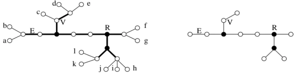
In Figure 1, a 2-branched partitioning-tree (T, R, σ) of the set {a, b, · · · , k, l} is
repre-sented. The vertex V ∈ V (T ) defines the partition TV = {abf ghijkl, c, de}, R ∈ V (T )
defines TR = {abcde, f g, hijkl}, and the edge E ∈ E(T ) defines the bi-partition
TE = {ab, cdef ghijkl}. The black vertices are the branching nodes of cp(T ).
E V R b a E c d V e f R g j i h k l
Figure 1: Partitioning-tree of {a, b, · · · , k, l} (left) and its corpse (right).
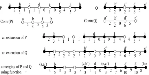
In Figure 2, we illustrate two labeled paths P and Q. The black vertices and bold
edges of P and Q are those that are represented in Contr(P ) and Contr(Q). The vertices of Contr(P ) and Contr(Q) are named as the vertices they represent in P and Q. We also illustrate an extension P∗ of P and an extension Q∗ of Q. The black
vertices and bold edges of P∗ and Q∗ are those in Init(P∗) and Init(Q∗). Finally, we
represent a merging of P and Q using the function F : (x, y) → x + y. When merging P and Q, we assume they have same ends, i.e., a = a′ and h = e′. The black vertices
and bold edges the merging R are those in M atching(R).
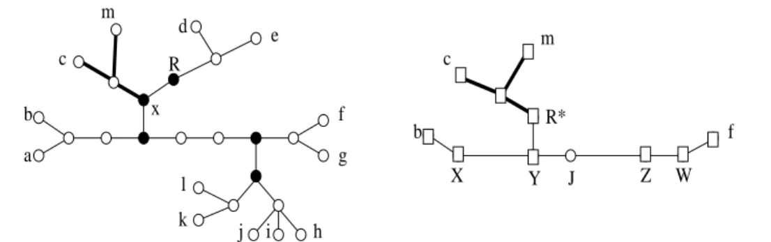
In Figure 3, we illustrate the building of the restriction of a partitioning-tree (T, R, σ)
of A = {abcdef ghijkl} to B = {bcf }. T is represented to the left of Figure 3. The black vertices are the branching nodes of cp(T ). We omit the labels of edges for a better readability.
The top-right figure represents the smallest subtree spanning the leaves of T that map elements of B (Step 1 of the building of Char((T, R, σ), B)). At Step 2, dist∗= 1. The
vertices represented by a square are the vertices of K∗ (Step 3). During Step 4, we set
branch∗(Y ) = branch∗(Z) = 1 and branch∗(R∗) = branch∗(X) = branch∗(W ) = 0,
and out∗(Z) = 1 and out∗(R∗) = out∗(Y ) = out∗(X) = out∗(W ) = 0.
Finally, during Step 6, any path P between two vertices in K∗, and with no internal
vertex in K∗ is replaced by Contr(P ). The bottom-right figure represents the final
an extension of P an extension of Q (c,b’) (e,c’) f d’ (h,e’) b d g (a,a’) a merging of P and Q using function a b 3 2 1 h 3 g 5 f 5 4 e 0 1 0 d 1 1 c 1 1 1 1 1 4 4 Q 2 0 5 b’ c’ e’ a’ 2 2 2 2 2 2 2 2 0 0 2 5 5 d’ 6 2 2 a b c d e f g h 5 5 1 1 3 1 2 1 1 0 0 4 3 P Contr(P) a b 3 2 0 Contr(Q) a’ b’ c’ d’ e’ 0 6 2 2 2 2 5 a’ b’ 0 2 2 d’ e’ 6 5 f 5 3 h 5 3 1 4 3 3 3 3 3 1 0 3 2 7 6 10 9 10 8
+
Figure 2: Labeled paths: contraction, extension and merging.
b c f R* b a c f g k l j i h R b c f R* e d E Y J Z W X 2 3 1 5 3 2 5 5 3 3 2 2 2 2 3 5 3 1 X I Y J K Z W 2
Figure 3: Partitioning-tree (T, R, σ) of {abcdef ghijkl} (left) and Char((T, R, σ), B), its characteristic restricted to {bcf } (bottom-right).
Figure 4 (left) illustrates the procedure of insertion that turns the partitioning-tree
(T, R, σ) (Figure 3 left) into a partitioning-tree (S, RS, σS) of A ∪ {m}. We choose
to illustrate the case when the insertion is performed by subdividing an edge E = {x, y} ∈ E(T ) (x is the parent of y). The bold edges are the new edges. Moreover, we are in the case when y is a leaf and x has exactly one non-leaf child in T . Therefore, x becomes a branching node of cp(S) in the new partitioning-tree.
Figure 4 (right) illustrates the same operation in Char((T, R, σ), B) (Figure 3 bottom-right). That is, Figure 4 (right) illustrates Procedure IntroduceN ode executed on an introduce node v of a nice decomposition D, such that, v has one child u, Xv =
b a f g k l i h R e d j c m b R* f c m x Y J Z W X
Figure 4: Insertion of {m} in (T, R, σ) by subdividing E (left). Same operation in Char((T, R, σ), B) (right).
Figure 5 represents the merging of a partitioning-tree (T, R, σ) of A∪B = {abcdef ghijkl}
(top-left) and a partitioning-tree (S, RS, σS) of A ∪ C = {bcf gmnopqrst} (top-right),
with A = {bcf g}. The bold edges are the edges of the smallest subtrees T′ and S′
(of T and S) spanning the leaves that map elements of A. The black vertices are the vertices of the common structure Struct of T and S obtained by contracting all degree-2 vertices of T′ and S′. Recall we also impose that R
S ∈ V (T′).
The graph in the middle results of the identifying of the vertices in this common structure. Now, any edge in Struct corresponds to two paths in the current graph. We compute a merging of these paths. A possible result is illustrated Figure 5 (bottom).
B
On labeled paths.
Let Φ be a monotone partition function. Any partitioning-tree (T, σ) can be viewed as a labeled graph, where any v ∈ V (T ) is labeled with Φ(Tv) and any e ∈ E(T ) is labeled with
Φ(Te). Because Φ is monotone, the label of an edge is at most the label of its ends. In
this section, we detail operations over labeled paths, that will serve as subroutine in the forthcoming sections.
B.1
Labeled paths.
A labeled path P is a path {v0, v1, · · · , vn} where any vertex vi is labeled with an integer
ℓ(vi), and any edge ei= {vi−1, vi} with an integer ℓ(ei). We assume moreover that the label
of any edge is at most the minimum label of its ends.
A vertex vi∈ V (P ) or an edge {vi, vi+1} is smallest than vj ∈ V (P ) if i < j. Similarly
vi (resp., {vi, vi+1}) is smallest than {vj, vj+1} if i < j. We define max(P ) as the maximum
integer labeling an edge or a vertex of P . Similarly, we define min(P ). An extension of a labeled path P is any path obtained by subdividing some edges of P an arbitrary number of times. Both edges and the vertex resulting from the subdivision of an edge e are labeled with ℓ(e). Let P∗be an extension of P . The initial elements Init(P∗) ⊆ V (P∗)∪E(P∗) of P∗are
a c f g b c f g b k l j i h e d b f g c k l j i h e d a b f g c e d a k l j i h m n R’ o p t s r q R n p o m t s r q m t s r q n p o R’
Figure 5: Merging of a partitioning-tree (T, R, σ) of A ∪ C = {abcdef ghijkl} and a partitioning-tree (S, RS, σS) of B ∪ C = {bcf gmnopqrst}, with C = {bcf g}.
the vertices of P∗ that do not result from the subdivision of an edge in P , and the edges of
P∗the smallest end of which are in Init(P∗). Given two labeled paths P and Q, we say that
P ¹ Q if there is an extension P∗= {p
1, · · · , pr} of P and an extension Q∗ = {q1, · · · , qr}
of Q with same length, and such that ℓ(pi) ≤ ℓ(qi) and ℓ({pi, pi+1}) ≤ ℓ({qi, qi+1}) for any
i ≤ r. For any function F : N → N, let F (P ) denote the path {v0, v1, · · · , vn, vn+1} where
any label ℓ has been replaced by F (ℓ). If P = {v1, · · · , vn} and Q = {w1, · · · , wm} are two
labeled paths with a common end vn = w1and vertex disjoint otherwise, their concatenation
B.2
Contraction of a labeled path.
In this section, we define an operation on labeled paths that will be widely used in the next sections. For this purpose, we revisit the notion of typical sequence of a sequence of integers [BK96]. Roughly, the goal of the following operation is to contract some edges and vertices of P that are not “necessary” to remember the variations of the sequence (ℓ(v0), ℓ(e1), ℓ(v1), · · · , ℓ(en), ℓ(vn)).
First, let us recall the definition of the typical sequence of a sequence of integers [BK96]. Let S = (si)i≤2n−1 be a sequence of integers. Its typical sequence τ (S) is obtained by
iterating the following operations while it is possible: (1) if there is i < |S| such that si = si+1, remove si+1 from S, and (2) if there are i < j − 1 < |S|, and either, for any
i ≤ k ≤ j, si ≤ sk ≤ sj, or, for any i ≤ k ≤ j, si ≥ sk ≥ sj, remove sk from S for any
i < k < j. Note that the order in which the operations are executed is not relevant, therefore τ (S) is uniquely defined.
The contraction Contr(P ) is the path obtained from P , with same ends, by contracting some edges and vertices obtained by the following procedure. Start with one integral variable m = 1. While m 6= n, do the following. Let i, m ≤ i ≤ n − 1, be the greatest index such that, for any m ≤ j ≤ i, ℓ(em) ≤ ℓ(ej)) ≤ ℓ(vi) and ℓ(em) ≤ ℓ(vj)) ≤ ℓ(vi). Contract all
vertices and edges between e and vi. Then, set m to the greatest index such that, for any
i < j ≤ m, ℓ(vi) ≥ ℓ(ej) ≥ ℓ(em) and ℓ(vi) ≥ ℓ(vj) ≥ ℓ(em). Contract all vertices and edges
between vi and em. Edges and vertices of Contr(P ) keep their initial label (cf. Figure 2 in
Appendix A).
The crucial property of Contr(P ) = {v0= v′0, v1′, · · · , vp−1′ , vp′ = vn} is that the sequence
S′ = (ℓ(e′
1), ℓ(v1′), · · · , ℓ(e′p−1), ℓ(vp−1′ ), ℓ(e′p)) (where e′i = {vi−1′ , vi′}) is “almost” the
typi-cal sequence of the sequence S = (ℓ(e1), ℓ(v1), · · · , ℓ(en)). More precisely, if ℓ(e′1) 6= ℓ(v1′),
then S′ = τ (S), otherwise (ℓ(v′
1), ℓ(e′2), · · · , ℓ(vp−1′ ), ℓ(e′p)) = τ (S) (τ (S) denotes the
typ-ical sequence of S). Moreover, it is important to note that any v ∈ V (Contr(P )) (e ∈ E(Contr(P ))) represents a unique v∗∈ V (P ) (e∗∈ E(P )).
Lemma 1. Let P and Q be two labeled paths. Let P∗ be an extension of P .
1. Contr(P∗) = Contr(P ) = Contr(Contr(P )).
2. Let F : N → N be any strictly increasing function. Contr(F (Contr(P ))) = Contr(F (P )). 3. If P ¹ Q, then Contr(P ) ¹ Contr(Q).
4. Contr(P ⊙ Q) = Contr(Contr(P ) ⊙ Contr(Q))
Lemma 2. Let P = {v0, · · · , vn} be a labeled path and Contr(P ) = {w0, · · · , wp}. Let
i ≤ p. Let Contr′(P ) = {w
0, · · · , wi, x, wi+1, · · · , wp} be the extension of Contr(P ) obtained
by subdividing once ei = {wi, wi+1}. Let e∗i = {vj, vj+1} be the edge of P represented by ei,
and P′= {v
0, · · · , vj, y, vj+1, · · · , vn} be the extension of P obtained by subdividing once e∗i.
Let Q1= {w0, · · · , x}, Q2= {x, · · · , wp}, P1′ = {v0, · · · , y} and P2′ = {y, · · · , vn}.
Then Contr(P′
B.3
Merging of labeled paths.
Now, we present an operation that merges two labeled paths P = {v1, · · · , vn} and Q =
{w1, w2, · · · , wm} with common ends (i.e., v1 = w1 and wm = vn) and vertex-disjoint
otherwise. For any i < n, ei = {vi, vi+1}, and for any i < m, fi = {wi, wi+1}. Let F : N ×
N→ N. Let P∗= {p
1, · · · , ph} be an extension of P and Q∗= {q1, · · · , qh} be an extension
of Q with same length. A merging R of P and Q using F is the labeled path {r1, · · · , rh},
where ri is labeled F (ℓ(pi), ℓ(qi)) and {ri, ri+1} is labeled F (ℓ({pi, pi+1}), ℓ({qi, qi+1})). We
say that ri matches pi = P eer(qi) ∈ V (P∗) and qi = P eer(pi) ∈ V (Q∗), and {ri, ri+1}
matches {pi, pi+1} = P eer({qi, qi+1}) ∈ E(P∗) and {qi, qi+1} = P eer({pi, pi+1}) ∈ E(Q∗).
Let M atching(R) be the set of pairs (pi, qi) such that pi∈ Init(P∗) or qi∈ Init(Q∗), and
the pairs ({pi, pi+1}, {qi, qi+1}) such that {pi, pi+1} ∈ Init(P∗) or {qi, qi+1} ∈ Init(Q∗).
Let R∗ be a merging of Contr(P ) and Contr(Q) using F . We say that a merging R of
P and Q respects R∗ if, for any (a, b) ∈ M atching(R∗), (a′, b′) ∈ M atching(R) where a′ is
the element of P represented by a in Contr(P ), and b′ is the element of Q represented by b
in Contr(P ).
Let us assume P = P1⊙ P2⊙ · · · ⊙ Pr, i.e., P = {v1, · · · , vn}, 1 = t1< t2< · · · < tr= n
are r integers, and Pi= {vti, · · · , vti+1}, i < r. Moreover, Q = Q1⊙ Q2⊙ · · · ⊙ Qq, that is,
Q = {w1, · · · , wm}, 1 = t′1 < t2′ < · · · < t′q = m are q integers, and Qi = {wt′
i, · · · , wt′i+1},
i < q. Any merging M of P and Q will be noted M = M1 ⊙ M2⊙ · · · ⊙ Mr, where
M = {y1, · · · , yk}, k1< · · · < kr are the indexes such yki matches a vertex vtj, j ≤ r, with
P eer(vtj), or yki matches a vertex wt′j, j ≤ q, with P eer(wt′j), and Mi = {yki, · · · , yki+1}
for any i < u.
Lemma 3. Let F : N × N → N strictly increasing on both coordinates. Let P = P1⊙ P2⊙
· · ·⊙Prand P′ = Contr(P1)⊙Contr(P2)⊙· · · ⊙Contr(Pr). Let Q = Q1⊙Q2⊙· · ·⊙Qq and
Q′= Contr(Q
1)⊙Contr(Q2)⊙· · · ⊙Contr(Qq). Let M′= M1′⊙M2′⊙· · ·⊙Mr′ be a merging
of P′ and Q′ using F , and let M = M
1⊙ M2⊙ · · · ⊙ Mr be a merging of P and Q using F
that respects M′. Then, Contr(M′
1) ⊙ · · · ⊙ Contr(Mr′) = Contr(M1) ⊙ · · · ⊙ Contr(Mr).
Moreover, if P′′ = P′′
1 ⊙ P2′′⊙ · · · ⊙ Pr′′, with Pi′′ ¹ Contr(Pi) for any i ≤ r, and
Q′′= Q′′
1⊙ Q′′2⊙ · · · ⊙ Q′′q, with Q′′i ¹ Contr(Qi) for any i ≤ q. Then, there is a merging
M′′= M′′
1 ⊙ · · · ⊙ Mr′′ of P′′ and Q′′ using F , such that Mi′′¹ Contr(Mi′) for any i ≤ r.
C
Proof of Lemma 7: Introduce node
Since Φ is closed under taking subset, Avadmits a q-branched partitioning-tree with Φ-width
at most k only if Au does. Therefore, we can assume that F SC(u) 6= ∅, otherwise, Av does
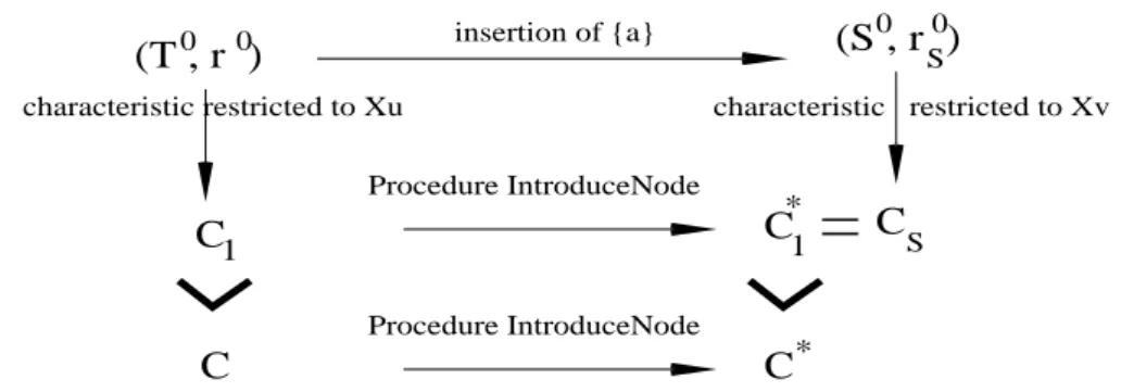
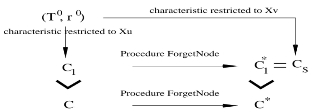
not admit a q-branched partitioning-tree with Φ-width at most k, and F SC(v) = ∅. The proof is twofold. We first prove that the set F SC(v) returned by Procedure IntroduceN ode is a set of characteristics of Av restricted to Xv, then we prove it is full. The proof is
(T , r )
0 0 0 0(S , r )
S Procedure IntroduceNode Procedure IntroduceNode characteristic restricted to XuC
* *C
insertion of {a}C
1C
1=
C
S characteristic restricted to XvFigure 6: Proof of correctness of Procedure IntroduceN ode
C.1
F SC
(v) is a set of characteristics of A
vrestricted to
X
vLet C∗
1 = ((T1∗, r∗1, σ1∗), ℓ∗1, K1∗, dist∗1, out∗1, branch∗1) ∈ F SC(v).
Let C1 = ((T1, r1, σ1), ℓ1, K1, dist1, out1, branch1) ∈ F SC(u) be the characteristic
trans-formed by procedure IntroduceN ode to compute C∗
1. Since C1∈ F SC(u), it is the
charac-teristic of a partitioning-tree (T0, r0, σ0) of A
u restricted to Xu. We prove that C1∗ is the
characteristic of the partitioning-tree (S0, r0
S, σ0S) of Av restricted to Xv, where (S0, r0S, σ0S)
is obtained from (T0, r0, σ0) by inserting {a} = X
v\ Xu.
We assume that C∗
1 is obtained from C1by inserting {a} in the edgef = {vtop, vbottom}.
This corresponds to Case 2 of Step 1 of Procedure IntroduceN ode. Case 1 can be proved in a similar way, and then we omit the proof here.
f ∈ E(T1), therefore, by definition of a characteristic, it represents an edge f0∈ E(T0).
Let (S0, r0
S, σ0S) = ins((T0, r0, σ0), f0, a), and let CS= ((TS, rS, σS), ℓS, KS, distS, outS, branchS) =
Char((S0, r0
S, σ0S), Xv) be its characteristic restricted to Xv. We prove that C1∗= CS.
We first prove that K∗
1 = KS. Indeed, let S′ be the smallest subtree of S0the leaves of
which map Xv, and let r′S be the vertex in S
′ that is closest to r0
S. KS is the set of vertices
that are leaves in (S′, r′
S), parents of leaves, branching nodes of (S
′, r′
S) or branching nodes
of cp(S0) in V (S′). Moreover, let T′ be the smallest subtree of T0 the leaves of which map
Xu, and let r′ be the vertex in T′ that is closest to r0. Since S0 is obtained from T0 by
subdividing f0 and adding a new leaf vleaf adjacent to the new vertex vatt, and moreover,
vleaf maps {a}, S′is obtained from T′by subdividing f0. Therefore, KS is the set of vertices
that are leaves in (T′, r′), or parents of leaves, or branching nodes of (T′, r′) or branching
nodes of cp(T0) in V (T′), or v
att or vleaf. In other words, KS = K1∪ {vatt, vleaf} = K1∗
(Step 1 of Procedure IntroduceN ode). Then, we prove that T∗
1 = TS and ℓ∗1 = ℓS. TS is obtained in the following way. Any
t ∈ V (S0) defines a partition S0
t of Av and receives label ℓ0(t) = ΦAv(S
0
t). Similarly,
any e ∈ E(S0) defines a partition S0
e of Av and receives label ℓ0(e) = ΦAv(S
0
e). Then,
TS is obtained from TS′ by replacing any path P (x, y) between two vertices x, y ∈ KS by
Contr(P (x, y)). Because KS = K1∗, x, y ∈ K1∗. Let us describe the path P1∗(x, y) between x
and y in T∗