Classifiers combination for recognition score improvement

HAL Id: inria-00107624

https://hal.inria.fr/inria-00107624

HAL is a multi-disciplinary open access archive for the deposit and dissemination of sci-entific research documents, whether they are

pub-L’archive ouverte pluridisciplinaire HAL, est destinée au dépôt et à la diffusion de documents scientifiques de niveau recherche, publiés ou non,

Classifiers combination for recognition score

improvement

Szilárd Vajda

To cite this version:

Szilárd Vajda. Classifiers combination for recognition score improvement. [Contract] A02-R-482 || vajda02c, 2002. �inria-00107624�

EDF PROJECT

Multi-oriented and multi-size alphanumerical character

recognition

PART III.

Classifiers combination for recognition score

improvement

This report corresponds to the task n.3 of the contract entitled: "Combinaison des classifieurs pour en améliorer les performances"

November 2002

Szilard VAJDA

1. Plan

• Objectives

• Combination methods description

• Experiments and results

• Conclusions

• References

2. Objectives

After the recognition step by using different kind of classifiers (MLP, SVM) and faced to the low recognition rates due to the bad quality of the database, it seemed natural to us, to combine the previous classifiers in order to improve the general recognition rate.

In fact, we cannot act individually on each classifier, because each classifier has shown its limits. Furthermore, the database drawbacks (low represented classes, bad quality of the character images, multi-scale and multi-size properties of the images) don’t allow to achieve better scores by using just only one classifier. So, the only remaining way to do it was to react, to merge many classifiers on the same samples for a best decision.

In the literature, a new trend called “Combination of multiple experts” (CME) has been developed in order to merge the different classifiers in a more powerful and more reliable one.

The main idea is to combine the different methods, different strategies with different features in order to complement each others. The cooperation between the different classification strategies and methods, conduces to an error reduction and achievement of a higher performance by the group decision.

In this work, we made experiments with two CME methods, wherewith were obtained good results in handwritten number recognition.

In the case of Stacked generalization method, the main idea is to use the output of a classifier as input for another classifier while in the Behaviour Knowledge Space method which operates in a behaviour knowledge space the result is derived from this space.

3. CME methods description

3.1. Method 1: Stacked generalization

The stacked generalization is a scheme for minimizing the error rate of one or more generalizers. Stacked generalization works by deducing the biases of the generalizer(s) with respect to a provided learning set. This deduction proceeds by generalizing in a second space whose input are the guesses of the original generalizers. When is used for multiple generalizers, stacked generalization can be seen as a more sophisticated version of cross-validation, exploiting a strategy more sophisticated than cross-validation’s crude winner-takes-all for combining the individual generalizers. The method will be presented through a scheme.

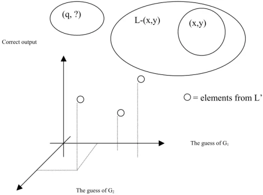
Figure 1: Stacked generalization method for two classifiers

In the scheme presented before (Figure 1) we can find the stacked generalization in the case of two generalizers, G1 respectively G2. The learning set L is represented by

the full ellipse. A question q is lying outside of L is also indicated. Finally, a partition of L is also indicated; one portion consists of the single input-output pair (x,y) and the other portion is contains the rest of L.

The guess of G2 L-(x,y) _(x,y) The guess of G1 Correct output = elements from L’ (q, ?)

Given this partition, we train both G1and G2 on the portion {L-(x,y)}. Then we ask

both generalizers the question x; their guesses are g1 and g2. In general, since the

generalizers have been not trained with the pair (x,y), both g1 and g2 will differ from

y. Therefore we just learned something; when G1guesses g1 and G2guesses g2, the

correct answer is y. This information can be cast as input-output information in a new space (i.e. as a single point with the 2-dimensional input (g1, g2) and the output y).

Choosing other partitions of L gives us other such points. Taken together, this points can be imagined as being a new learning set L’. We train our generalizers G1 and G2

on all of L and ask them both the question q. By having their guesses, we feed that pair as a question to a third generalizer, which has been trained on L’. This third generalizer’s guess is our final guess for what output corresponds to q.

3.2. Method 2: Behaviour Knowledge Space

The most of the CME methods require the independence assumption, by this we mean to treat each classifier equally or to derive useful information for the combination stage from the confusion matrix of a single classifier. To avoid this assumption, the information should be derived from a knowledge space which can concurrently record the decisions of all classifiers on each learned sample. Since this knowledge space records the behaviour of all classifiers, it is called “Behaviour Knowledge Space” (BKS).

A BKS is a K-dimensional space, where each dimension corresponds to the decision of one classifier. Each classifier has M+1 possible decision values. The intersection of individual classifiers occupies one unit in BKS which is called focal unit. Each unit contains three kind of data:

• the total number of incoming samples • the best representative class

• the total number of incoming samples for each class Symbols used in defining a BKS are:

BKS =a K-dimensional behaviour-knowledge space

BKS(e(1),e(2),…e(K)) =a unit of BKS, where classifier 1 gives its decision as e(1),...,and classifier K gives its decision as e(K).

ne(1)…e(K)(m) =the total number of samples belonging to class m in

BKS(e(1),e(2),…e(K))

T(e(1),e(2),…e(K)) =the total number of incoming samples in BKS(e(1),e(2),…e(K)) =

¦

R(e(1),e(2),…e(K)) =the best representative class of BKS(e(1),e(2),…e(K)) =

{

}

The BKS operates in two stages: knowledge modelling and decision making. The knowledge modelling stage uses the learning samples with genuine and recognized class labels to construct the BKS; then the values of T(e(1),e(2),…e(K)) and R(e(1),e(2),…e(K)) are computed as presented before.

The decision making process according to the built BKS and the individual decision of the classifiers, enters the focal unit and makes the final decision by the following rule: ° ¯ ° ® ­ + ≥ = otherwise M T R n and whenT R x E _{e eK} K e e K e e K e e K e e , 1 ( 0 ) ( ) ( )... 1 ( ) ( )... 1 ( ) ( )... 1 ( ) ( )... 1 ( ) ( )... 1 ( λ

4. Experiments and results

4.1. Stacked generalization method results

We used this method, in both ways, to improve a single model (in our case the MLP and the SVMs) and respectively to improve the results of both classifiers together. As was presented before, with this method we are projecting our samples in a lower dimension space, where we are using another classifier to make the final decision. In our case each time the 2nd classifier was a MLP with one hidden layer.

4.1.1. Improvement of a single classifier with stacked generalisation method

In the MLP’s case we used the answers of the MLP in order to create a 2nd low dimension space (62 inputs) and we used as 2nd classifier, an another MLP with one

hidden layer (124 units) in order to improve the results. In that case we obtained 73,45% which is an amelioration of 3,98%

The same procedure with the results of the SVMs generated an amelioration of 0,5%.

4.1.2. Improvement of the MLP and SVMs by a hybrid stacked generalization

In that case we used the outputs coming from the SVMs and the images (shape matrices) which were used in the first case (see Training and evaluation of the models for isolated character recognition). For this joint process we used a 2nd MLP with 638 inputs (the outputs of the SVMs(62) and the shape matrices(576)), 212 units in the hidden layer and respectively 62 neurons in the output. The MLP was fully connected. In that case we obtained 77,48% which is an amelioration of 8,01%. In that case we used no rejection criteria, each character was recognised as an alphanumerical character and it was not used any kind of regroupment operation. In order to make the decision more precisely, we introduced a rejection criteria and a regroupment too.

We used as rejection criteria, the fact than the distance between the first two possible candidates in the output layer of the MLP should have a distance ∆dbetween them in order to make our final decision, if not, we are rejecting the character.

As regroupment operation we used the fact, than some characters are very similar, so we should treat them as one. We used the following regroupment operations: {0,o,O,D}=0, {2,z,Z}=2, {1,i,l,I,J}=1, {8,B}=8, {c,C}=C, {p,P}=P, {u,U}=u, {s,S}=S, {v,V}=V, {x,X}=x. By introducing these operators, we reduced the number of classes, from 62 to 53.

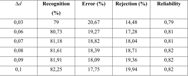
By making the regroupment operations, we achieved 85,24% recognition score. In the next two tables, we are presenting the results achieved by using the rejection criteria and no kind of regroupment operation and respectively the result obtained with regroupment and rejection criteria.

d

∆ Recognition (%)

Error (%) Rejection (%) Reliability

0,03 79 20,67 14,48 0,79 0,06 80,73 19,27 17,28 0,81 0,07 81,18 18,82 18,04 0,81 0,08 81,61 18,39 18,71 0,82 0,09 81,91 18,09 19,36 0,82 0,1 82,25 17,75 19,94 0,82

Table 1: Recognition results with rejection

d

∆ Recognition (%)

Error (%) Rejection (%) Reliability

0,08 88,31 11,69 18,71 0,88 0,09 88,48 11,52 19,36 0,88 0,1 88,72 11,28 19,94 0,88

Table 2: Recognition results with rejection and regroupment

4.2. Behaviour Knowledge Space method results

In this case, as was presented in chapter 3.2, we created the BKS space and after we made our decision by the rule presented here. In the building phase of the BKS space it was used the results of the MLP respectively the SVMs.

Without any kind of regroupment and rejection criteria, we achieved 70,93% as recognition score.

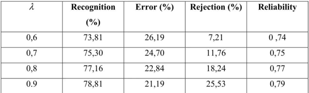
In the next table we are presenting the results obtained with the use of the rejection criteria in the BKS case.

λ Recognition (%)

Error (%) Rejection (%) Reliability

0,6 73,81 26,19 7,21 0 ,74 0,7 75,30 24,70 11,76 0,75 0,8 77,16 22,84 18,24 0,77 0.9 78,81 21,19 25,53 0,79

Table 3: Recognition results with rejection

5. Conclusions

In the tables below, we can find the comparisons between two combinational models used in the experiments. As we can see, the Stacked generalization is giving betters results than the BKS.

Method (no regroupment, no rejection) Recognition(%) Stacked generalization 77,48

BKS 70,93

Table 4: Comparison between Stacked generalization and BKS without rejection and without regroupment

The cause of result differences between these methods can be explained with the different way of acting (see decision making) of the classifiers. As long as in the Stacked generalization case, the classifier it’s able to learn from that low dimensional space, in the second case, the classification criteria is more rigid.

By introducing the rejection criterions we can see, the same proportions in the recognition scores.

Method (no regroupment, rejection) Recognition(%) Stacked generalization 88,72

BKS 78,81

Table 5: Comparison between Stacked generalization and BKS with regroupment and without regroupment

By using in the BKS method, more classifiers, as elementary classifiers (see ei), the

BKS space will become more complex, by this way it will be possible to make more complex and precisely decisions in that space too.

Taking in consideration the results, obtained by the combination of the classifiers (MLP and SVMs), we consider these results as been successfully.

The bad quality of the database, the low representation of some classes and the different orientations and size of the characters are limiting the recognition process to this layer.

As future works, we are proposing the usage of other elementary classifiers, in order to give enough information to the CME models and another considered aspect would be the usage of the rotation angle of the characters, which will simplify the work of the MLP, which is sensitive to the geometrical transformations.

Another aspect, could be the improuvement of the Goshtasby transform, by introducing a more precise building technique of the shape matrix and the perfection of the shifting technique.

6. References

[1] Y. S. Huang, C. Y. Suen, “A method of combining multiple experts for the recognition of unconstrained handwritten numerals”, IEEE Transactions on Pattern Recognition and Machine Intelligence, vol. 17, no. 1, January 1995

[2] David H. Wolpert, “Stacked generalization”, Neural Networks, vol. 5, 241-259, 1992