HAL Id: inserm-02965257
https://www.hal.inserm.fr/inserm-02965257
Submitted on 13 Oct 2020
HAL is a multi-disciplinary open access archive for the deposit and dissemination of sci-entific research documents, whether they are pub-lished or not. The documents may come from teaching and research institutions in France or abroad, or from public or private research centers.
L’archive ouverte pluridisciplinaire HAL, est destinée au dépôt et à la diffusion de documents scientifiques de niveau recherche, publiés ou non, émanant des établissements d’enseignement et de recherche français ou étrangers, des laboratoires publics ou privés.
effects of regional stimulation depend on collective
dynamical state
Lia Papadopoulos, Christopher Lynn, Demian Battaglia, Danielle Bassett
To cite this version:
Lia Papadopoulos, Christopher Lynn, Demian Battaglia, Danielle Bassett. Relations between large-scale brain connectivity and effects of regional stimulation depend on collective dynamical state. PLoS Computational Biology, Public Library of Science, 2020, 16 (9), pp.e1008144. �10.1371/jour-nal.pcbi.1008144�. �inserm-02965257�
RESEARCH ARTICLE
Relations between large-scale brain
connectivity and effects of regional
stimulation depend on collective dynamical
state
Lia Papadopoulos1, Christopher W. Lynn1, Demian BattagliaID2, Danielle S. BassettID1,3,4,5,6,7
*
1 Department of Physics & Astronomy, University of Pennsylvania, Philadelphia, Pennsylvania, United States
of America, 2 Universite´ Aix-Marseille, INSERM UMR 1106, Institut de Neurosciences des Systèmes, F-13005, Marseille, France, 3 Department of Bioengineering, University of Pennsylvania, Philadelphia, Pennsylvania, United States of America, 4 Department of Electrical & Systems Engineering, University of Pennsylvania, Philadelphia, Pennsylvania, United States of America, 5 Department of Neurology, University of Pennsylvania, Philadelphia, Pennsylvania, United States of America, 6 Department of Psychiatry, University of Pennsylvania, Philadelphia, Pennsylvania, United States of America, 7 Santa Fe Institute, Santa Fe, New Mexico, United States of America
*dsb@seas.upenn.edu
Abstract
At the macroscale, the brain operates as a network of interconnected neuronal populations, which display coordinated rhythmic dynamics that support interareal communication. Understanding how stimulation of different brain areas impacts such activity is important for gaining basic insights into brain function and for further developing therapeutic neurmodula-tion. However, the complexity of brain structure and dynamics hinders predictions regarding the downstream effects of focal stimulation. More specifically, little is known about how the collective oscillatory regime of brain network activity—in concert with network structure— affects the outcomes of perturbations. Here, we combine human connectome data and bio-physical modeling to begin filling these gaps. By tuning parameters that control collective system dynamics, we identify distinct states of simulated brain activity and investigate how the distributed effects of stimulation manifest at different dynamical working points. When baseline oscillations are weak, the stimulated area exhibits enhanced power and frequency, and due to network interactions, activity in this excited frequency band propagates to nearby regions. Notably, beyond these linear effects, we further find that focal stimulation causes more distributed modifications to interareal coherence in a band containing regions’ baseline oscillation frequencies. Importantly, depending on the dynamical state of the system, these broadband effects can be better predicted by functional rather than structural connectivity, emphasizing a complex interplay between anatomical organization, dynamics, and response to perturbation. In contrast, when the network operates in a regime of strong regional oscillations, stimulation causes only slight shifts in power and frequency, and struc-tural connectivity becomes most predictive of stimulation-induced changes in network activ-ity patterns. In sum, this work builds upon and extends previous computational studies investigating the impacts of stimulation, and underscores the fact that both the stimulation
a1111111111 a1111111111 a1111111111 a1111111111 a1111111111 OPEN ACCESS
Citation: Papadopoulos L, Lynn CW, Battaglia D, Bassett DS (2020) Relations between large-scale brain connectivity and effects of regional stimulation depend on collective dynamical state. PLoS Comput Biol 16(9): e1008144.https://doi. org/10.1371/journal.pcbi.1008144
Editor: Daniele Marinazzo, Ghent University, BELGIUM
Received: February 15, 2020 Accepted: July 12, 2020 Published: September 4, 2020
Copyright:© 2020 Papadopoulos et al. This is an open access article distributed under the terms of
theCreative Commons Attribution License, which
permits unrestricted use, distribution, and reproduction in any medium, provided the original author and source are credited.
Data Availability Statement: The data used in this study is available from https://github.com/lia-papadopoulos/WilsonCowan_DynamicalState_ Stim.
Funding: This work was primarily supported by National Science Foundation BCS-1631550, Army Research Office W911NF-18-1-0244, and National Institutes of Health R01-MH -116920. DSB, LP, and CWL would like to acknowledge additional support from the John D. and Catherine T. MacArthur Foundation, the Alfred P. Sloan
site, and, crucially, the regime of brain network dynamics, can influence the network-wide responses to local perturbations.
Author summary
Stimulation can be used to alter brain activity and is a therapeutic option for certain neu-rological conditions. However, predicting the distributed effects of local perturbations is difficult. Previous studies show that responses to stimulation depend on anatomical (or structural) coupling. In addition to structure, here we consider how stimulation effects also depend on the brain’s collective dynamical (or functional) state, arising from the coordination of rhythmic activity across large-scale networks. In a whole-brain computa-tional model, we show that global responses to regional stimulation can indeed be contin-gent upon and differ across various dynamical working points. Notably, depending on the network’s oscillatory regime, stimulation can accelerate the activity of the stimulated site, and lead to widespread effects at both the new, excited frequency, as well as in a much broader frequency range including areas’ baseline frequencies. While structural connec-tivity is a good predictor of “excited band” changes, in some states “baseline band” effects can be better predicted by functional connectivity, which depends upon the system’s oscil-latory regime. By integrating and extending past efforts, our results thus indicate that dynamical—in additional to structural—brain organization plays a role in governing how focal stimulation modulates interactions between distributed network elements.
Introduction
The brain is a multiscale system composed of many dynamical units that interact to produce a vast array of functions. At a large scale, macroscopic regions—each containing tens of thou-sands of neurons—are linked by a physical web of white matter tracts that facilitate the propa-gation of activity between distributed network elements. At the level of large neuronal ensembles or brain areas, collective activity is often rhythmic in nature [1], and these rhythms can become temporally coordinated between distant regions, giving rise to so-called functional interactions [2]. Importantly, oscillations have been implicated in a number of cognitive pro-cesses [3–9], and coherent activity is hypothesized to play an important role in interareal com-munication and information transfer among distributed brain areas [5,6,10]. Nonetheless, despite progress in mapping and characterizing the brain’s anatomical pathways and measur-ing neural oscillations, a number of questions remain as to how individual components in a brain network shape and modulate system-wide dynamics.
Among these questions, understanding how large-scale, oscillatory brain dynamics respond to localized perturbations is of critical importance [7,11–14]. Because the brain is not a closed or static system, such activity changes could be induced by sensory inputs to pri-mary sensory areas [15,16], different tasks [17,18], or other internal or regulatory processes [19–22]. In addition to naturally-induced changes, stimulation techniques such as transcra-nial magnetic stimulation [23], direct current stimulation [24], and alternating current stim-ulation [25] can also be employed to invoke modulations of dynamics in a specific brain area. By combining these techniques with imaging methods like EEG and MEG [26–31], it is possible to examine how the act of exciting a particular network component modifies rhythmic neural activity. Furthermore, in addition to its utility for basic science,
Foundation, the ISI Foundation, the Paul Allen Foundation, the Army Research Laboratory (W911NF-10-2-0022), the Army Research Office (Bassett-W911NF-14-1-0679, Grafton-W911NF-16-1-0474, DCIST-W911NF-17-2-0181), the Office of Naval Research, the National Institute of Mental Health (2-R01-DC-009209-11, R01-MH112847, R01-MH107235, R21-M MH-106799), the National Institute of Child Health and Human Development (1R01HD086888-01), National Institute of Neurological Disorders and Stroke (R01 NS099348), and the National Science Foundation (BCS-1441502, BCS-1430087, and NSF PHY-1554488). LP was also supported by a Graduate Research Fellowship from the National Science Foundation for part of this work. DB acknowledges support from the EU i-Innovative Training Network “i-CONN” (H2020 MSCA ITN 859937) and the French Agence Nationale pour la Recherche (“ERMUNDY”, ANR-18-CE37-0014-02). The content is solely the responsibility of the authors and does not necessarily represent the official views of any of the funding agencies. The funders had no role in study design, data collection and analysis, decision to publish, or preparation of the manuscript.
Competing interests: The authors have declared that no competing interests exist.
neurostimulation has emerged as a promising approach for treating a number of neurologi-cal and psychiatric conditions [32–34].
Yet, while prior work has often focused on characterizing the proximal effects of local per-turbations, a growing body of literature indicates that regional changes to neural activity can have more widespread consequences [11–14]. The realization that stimulation can have net-work-wide effects necessitates further investigations into the operating principles underlying such phenomena [35–42]. Furthermore, a crucial but seemingly understudied point is that the effects of perturbing a particular brain area can depend not only on the nature or location of the perturbation, but also on the intrinsic dynamical state of the system at baseline [43–45]. In particular, recent efforts have investigated the state-dependent effects of stimulation via precise experiments [46,47]—focusing largely on alpha-band activity in single cortical areas—and via modeling [48–50]. These studies have uncovered robust relationships between the endogenous state of rhythmic activity and the capacity of external stimulation to modulate cortical oscilla-tions in a given brain area. However, a pivotal next step is to extend the notion of state-depen-dence to the case of whole-brain networks, which acknowledge the fact that regions do not operate in isolation. Rather, in the case of large-scale brain networks, the macroscopic dynam-ical regime of the system arises from an interplay between units’ local activity and long-range anatomical coupling [51], leading to the emergence of collective oscillatory modes [40,52]. Although it is reasonable to hypothesize that the global state of brain network activity should play a role in determining how a focal perturbation will manifest and influence distributed functional interactions, these ideas have yet to be systematically examined.
Thus, there is now a need to concurrently investigate and merge two outstanding ques-tions:(1) how regional stimulation spreads to induce distributed effects on brain network
dynamics, and(2) how the global dynamical regime of the system impacts these effects. Here,
we investigate these questions by constructing a biophysically-motivated model of large-scale, oscillatory brain activity, in which individual brain areas are modeled as Wilson-Cowan neural masses [53] coupled according to empirically-derived anatomical connectivity [51]. We first demonstrate that, in the absence of stimulation, the interareal coupling strength and the baseline excitation of the network transition the system between qualitatively distinct collective dynamical states. By providing additional excitation to a single brain area, we then systematically examine the consequences of such local stimulation on network activity. The primary contribution of this study is an exploration of how the effects of focal perturbations can depend not only on which area is stimulated, but also on the baseline dynamical regime of the non-linear model. Hence, this work builds upon previous whole-brain modeling efforts that have examined the effects of regional perturbations [35–37] with other work examining the state-dependent effects of stimulation in single cortical areas, but not large-scale networks [48,49].
We find that in states of low baseline excitation, stimulation can significantly increase the frequency and power of regional activity, whereas in states of high background drive, local dynamics are less sensitive to perturbations. Importantly, these results show qualitative simi-larities and agreement with past work examining the focal effects of stimulation [48,49]. We further find that, due to network interactions, regional perturbations can propagate and inter-act with brain areas’ ongoing rhythms. In particular, depending on the system working point, downstream areas that are strongly anatomically linked to the stimulated site also develop spectral components at the excited frequency of the stimulated region. Crucially, though, mod-ifications to interareal phase-locking can additionally be induced in a broader frequency band comprising brain areas’ spontaneous, baseline oscillations, which may be well-separated from the excited frequency. Moreover, changing the dynamical regime of the system modulates the strength of associations between network-wide responses to perturbations in the baseline
frequency band and structural or functional network connectivity. Hence, changing the collec-tive oscillatory state of the system—which need not be entirely determined by the anatomical network—qualitatively changes the distributed effects of focal perturbations, and alters the relations between those effects and measures of either structural or dynamical organization. In sum, we use a simplfied, large-scale computational model to highlight that the effects of regional stimulation can depend both on the location of the perturbed site and on the global state of ongoing brain network dynamics. Though currently idealized, extending the reduced model to incorporate further biological realism and empirical constraints is an exciting direc-tion for future work attempting to directly compare against experimental findings.
Materials and methods
Acquisition of empirical human structural brain data
Human anatomical brain networks were reconstructed by applying deterministic tractography algorithms to diffusion-weighted MRI. In this study, we used a group-representative compos-ite network assembled from 30 subject-level networks [54–56]. The mean age of participants was 26.2 years, the standard deviation was 5.7 years, and 14 of the subjects were female. To map anatomical networks, diffusion spectrum and T1-weighted anatomical images were acquired for each individual. For the DSI scans, 257 directions were sampled using a Q5 half-shell acquisition scheme with a maximumb-value of 5000 s/mm2and an isotropic voxel size of 2.4 mm. We used an axial acquisition with repetition time TR = 5 seconds, echo time TE = 138 ms, 52 slices, and field of view of [231, 231, 125]mm. The T1 sequences used a voxel size of [0.9, 0.9, 1.0]mm, repetition time TR = 1.85 seconds, echo time TE = 4ms, and field of view of [240, 180, 160]mm. This data was initially collected for an earlier study [57], and was first pub-lished in [58]. The same data has also been used in several other prior investigations (e.g., [54,
56,59]).
DSI Studio (www.dsi-studio.labsolver.org) was used to reconstruct DSI data usingq-space
diffeomorphic reconstruction (QSDR) [60], which reconstructs diffusion-weighted images in native space and computes the quantitative anisotropy (QA) of each voxel. Using the statis-tical parametric mapping nonlinear registration algorithm [61], the image is then warped to a template QA volume in Montreal Neurological Institute (MNI) space. Finally, spin-density functions were reconstructed with a mean diffusion distance of 1.25 mm with three fiber ori-entations per voxel. A modified FACT algorithm [62] was then used to perform deterministic fiber tracking with an angular cutoff of 55˚, step size of 1.0 mm, minimum length of 10 mm, spin density function smoothing of 0.00, maximum length of 400 mm, and a QA threshold determined by DWI signal in the colony-stimulating factor [54–56,58,59,63]. The algorithm terminated when 1,000,000 streamlines were reconstructed for each individual [54–56,58,59,
63] (Fig 1A).
T1 anatomical scans were segmented using FreeSurfer [64] and parcellated using the Con-nectome Mapping Toolkit (http://www.connectomics.org) according to anN = 82 area atlas
[65] of 68 cortical and 14 subcortical areas (Fig 1B; Table A inS1 Text). The parcellation was registered to theb0 volume of each subject’s DSI data, and region labels were mapped from
native space to MNI coordinates using ab0-to-MNI voxel mapping [54–56,58,59,63]. While we use a relatively coarse-grained atlas, it aligns with atlas sizes used in other computational modeling studies (e.g., [35,66–69]),and was chosen to reduce the computational costs of numerical simulations. However, we do mention limitations involved with this choice in the Discussion.
Ethics statement. All participants gave informed consent in writing and all protocols
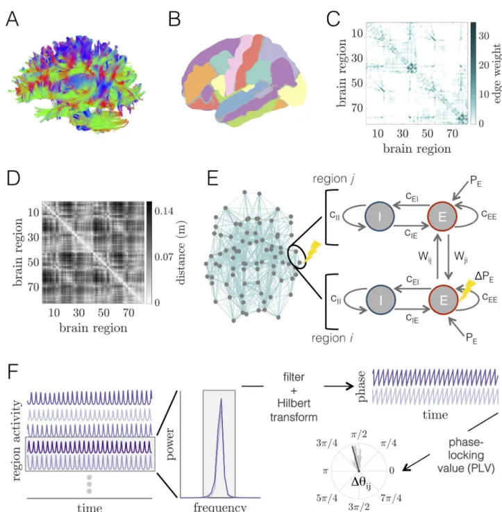
Fig 1. Whole-brain imaging data, computational model of large-scale brain dynamics, and schematic of analysis.(A) An example of white matter
streamlines reconstructed from diffusion imaging and tractography of a human brain.(B) Noninvasive magnetic resonance imaging scans of human
brain anatomy are used to segment the cortex and subcortex into 82 regions.(C) Adjacency matrix for a group-averaged structural brain network.
Individual brain areas are represented as network nodes, and normalized white matter streamline counts between region pairs are represented as weighted network edges.(D) Matrix of Euclidean distances between the centers of mass of all region pairs. (E) Left: Structural brain network
representation; location of gray circles correspond to region centers of mass, and teal lines show the strongest 20% of interareal connections, with line thickness proportional to connection strength. The two encircled nodes correspond to an unperturbed regionj and an excited region i in the large-scale
brain network, with the perturbed region indicated by the yellow lightning bolt. Right: Schematic of the computational model of large-scale brain dynamics. The activity of a given brain regionj is modeled as a Wilson-Cowan neural mass, composed of interacting populations of excitatory E and
inhibitoryI neurons. Neural masses are then coupled through their excitatory pools according to the structure of the anatomical brain network. A
perturbation to regioni (pictorially represented with the lightning bolt) is modeled as an increase in its excitatory input from PE!PE+ΔPE.(F) The
computational model generates oscillatory time-series of neural population activity for each brain region. These time-series can then be analyzed in Fourier space to determine relevant frequency bands for further analysis. After filtering time-series within the same frequency band of interest, functional interactions between brain region pairs are determined by extracting phase variables from each region’s filtered activity via the Hilbert transform, and then computing the phase-locking value to assess the consistency of phase relations over time and trials.
Network representation of anatomical brain data
To incorporate the structure of interareal connections into the model of large-scale brain activ-ity, we represented the anatomical brain data as a network. This was achieved by first mapping each of theN = 82 regions to a unique node in a structural brain network A (see Table A inS1 Textfor the mapping between node numbering and brain region labels). The structural edge weightAijbetween two brain areas (nodes)i and j was then defined as the total number of
streamlines between the two areas divided by the geometric mean of their volumes [54,56]. Note that due to limitations in the non-invasive techniques available for constructing human connectomes [70], the resulting structural network is weighted but undirected. Because the brain is a spatially-embedded system [71], each regioni also has a location ri= (xi,yi,zi) in real
space. In the network representation, we defined the location of each node to be the center of mass of the corresponding region, allowing us to calculate matrix elementsDijrepresenting
the Euclidean distance between nodesi and j. Assuming a fixed conduction speed, these
inter-areal distances are then used to approximate time delays for signal transmission in the compu-tational model [35,66,67,72,73].
In this study, we report results using a group-representative structural brain network derived by combining individual brain networks across multiple subjects. We used a previ-ously-established consensus method for constructing the group representative network that preserves both the average binary connection density of the individual brain networks, as well as the approximate edge-length distribution of intra- and inter-hemispheric connections [54]. More details on this pooling procedure can be found in [55]. A group-representative interareal distance matrix was constructed by averaging the pairwise Euclidean distance matrices across subjects. In what follows, we assume that A (orAij) refers to the group-representative
struc-tural brain network, and that D (orDij) refers to the group-averaged interareal distance matrix.
We show the group-representative anatomical connectivity matrix inFig 1C, and we show the group-averaged distance matrix inFig 1D.
Biophysical model of large-scale brain dynamics
To model large-scale brain dynamics, we use a biophysically-motivated approach in which simulated activity is generated by a network of interacting neural masses [51]. In particular, the activity of each brain area is modeled as a Wilson-Cowan (WC) neural mass [53] and indi-vidual units are coupled according to the empirically-derived anatomical network. Impor-tantly, these types of whole-brain computational models—which integrate non-linear, mean-field population dynamics with structural connectome architecture—have been utilized in a number of past efforts to gain insight into diverse neural phenomena [35,66,67,69,72–83].
Here, we employ such an approach to conduct a basic examination of how localized (regional) changes in neural activity affect dynamics across the brain. We offer a schematic of the model inFig 1E. On the left, we show the structural brain network in real space. We focus on the two interconnected regionsi and j encircled in black, of which the lower one (i) receives
additional excitation (as denoted by the yellow lightning bolt). On the right, we show the setup of the coupled WC system for these two units. In the WC model, the activity of a particular brain region is defined by a coupled system of excitatory (E) and inhibitory (I) neuronal
popu-lations, and the dynamical variables are the mean firing rates of theE and I pools. The
time-evolution of the average firing rates are in general governed by both intrinsic properties of the populations in a single region, as well as delayed, long-range input from other areas as dictated by the pattern of anatomical connectivity. In line with several previous studies [35,66,73–77,
81], we consider long-range connections to couple only the excitatory subpopulations of dis-tinct brain areas.
The dynamics of thejthbrain area are governed by the following set of coupled differential equations: tEdEjðtÞ dt ¼ EjðtÞ þ ½1 EjðtÞ�SE½cEEEjðtÞ cIEIjðtÞ þCX i WijEiðt tijÞ þPE;j� þ sExðtÞ ð1Þ and tIdIjðtÞ dt ¼ IjðtÞ þ ½1 IjðtÞ�SI½cEIEjðtÞ cIIIjðtÞ þPI;j� þ sIxðtÞ: ð2Þ
The variablesEj(t) and Ij(t) correspond to the firing rates of the excitatory and inhibitory
populations of regionj, and τEandτIare the excitatory and inhibitory time constants,
respec-tively. The non-linear activation functionsSEandSIof the excitatory and inhibitory pools are given by the sigmoidals
SEðxÞ ¼ 1
1 þe aEðx mEÞ ð3Þ
and
SIðxÞ ¼ 1
1 þe aIðx mIÞ: ð4Þ
The quantitiesμEandμIgive the mean firing thresholds for each subpopulation, and the
gain parametersaEandaIset the spread of the firing thresholds for the two groups.
Dynamics of the excitatory ensemble are driven by(1) the local interaction strength within
the excitatory populationcEE,(2) the interaction strength from the inhibitory population to
the excitatory populationcIE,(3) constant, non-specific background drive PE,j, and also(4)
interactionsWijcorresponding to long-range excitatory inputs from different populationsi
that link to unitj via anatomical connectivity. Following [75–77,84], we letWij¼ Aij
P
iAij
, which is simply the connection weight fromi to j, normalized by the total input to region j.
Further-more,C is a global coupling that tunes the overall interaction strength between different brain
areas, andτijis a time delay between regionsi and j that arises due to the spatial embedding of
the brain network and the fact that signal transmission speeds are finite [35,66,67,69,72,73]. We set tij¼Dij
v, whereDijis the Euclidean distance between regionsi and j and v is a constant
signal conduction speed. Activity in the inhibitory ensemble depends on(1) the interaction
strengthcEIfrom the excitatory population,(2) the local interaction strength within the
inhibi-tory populationcII, and(3) other possible non-specific inputs PI,j. Finally, to increase biological
plausibility and incorporate the stochastic nature of neural dynamics, we add a termσEξ(t) to
Eq 1and a termσIξ(t) toEq 2, which correspond to Gaussian white noise with zero mean and
standard deviationsσEandσI, respectively [35,73]. In what follows, we will take the excitatory
population activitiesEj(t) of each brain area as the observables of interest [35,66,75,76,83].
Model parameters. Under appropriate parameter choices, the WC model can give rise to
oscillatory dynamics [53]. Such rhythmic activity is ubiquitous in large-scale neural systems [1] and is the dynamical behavior of interest for this investigation. While oscillation frequen-cies observed in neural systems can span orders of magnitude [1], local neuronal populations
often exhibit gamma band (30-90Hz) rhythms as a result of feedback between coupled excit-atory and inhibitory neurons [4,85,86]. Furthermore, gamma oscillations and synchroniza-tion between distributed brain areas are associated with the flow of informasynchroniza-tion between neuronal ensembles [10,87,88], are modulated by stimuli [15,16], and are thought to underlie a number of cognitive processes [6]. Because gamma oscillations are robustly observed in excitatory-inhibitory circuits, we set parameters in the phenomenological WC model such that individual brain regions oscillate in the gamma band when coupled [73] (seeTable 1). We also note that it may be interesting in future work to investigate other frequency bands or multiple frequency bands simultaneously [89].
As discussed further in Sec. SI ofS1 Text, the non-specific background inputPEis the typical
control parameter used to tune the behavior of an isolated WC unit. At low values ofPE, a single
WC unit flows towards a low-activity steady-state (Fig. A, panel A inS1 Text), and at high val-ues ofPE, the system reaches a stable high-activity steady-state (Fig. A, panel C inS1 Text). At
intermediate values of the excitatory drive, an isolated unit—with the parameters given in
Table 1—will undergo a bifurcation and exhibit rhythmic activity in the gamma frequency band (Fig. A, panel B inS1 Text). Up to a point, increasingPEwithin this intermediate region
leads to oscillations with increasing amplitude and frequency (Fig. A, panels D–F inS1 Text). The situation becomes more complex when multiple WC units are coupled via the struc-tural connectome. In this scenario, an individual region’s dynamics are determined by a com-bination of the constant drivePEand the strength of delayed inputs from other parts of the
network, which are modulated by the couplingC and the structural connectivity A. To account
for these two influences, we consider bothPEandC as tuning parameters, and examine
work-ing points at which the combination ofPEandC generate oscillatory activity in individual
brain areas. Finally, we set the signal propagation speed to a fixed value ofv = 10m/s, which is
in the range of empirical observations and previous large-scale modeling efforts [35].
Table 1. Parameter values for the large-scale Wilson-Cowan neural mass model and for the numerical simulations.
Parameter Description Value
v propagation speed 10m/s
C global coupling strength 0–5
τE excitatory time constant 2.5ms
τI inhibitory time constant 3.75ms
aE excitatory gain 1.5
aI inhibitory gain 1.5
μE excitatory firing threshold 3.0
μI inhibitory firing threshold 3.0
cEE local E to E coupling 16
cIE local I to E coupling 12
cEI local E to I coupling 15
cII local I to I coupling 3
Pbase
E baseline excitatory background drive 0.5–0.85
ΔPE perturbation strength 0.1
PI inhibitory background drive 0
σE excitatory noise strength 5× 10⁻⁵
σI inhibitory noise strength 5× 10⁻⁵
dt integration time step 5× 10⁻⁵s
dtds downsampled time step 1× 10⁻³s
Incorporating local perturbations into the large-scale model. The baseline condition of
the network corresponds to the situation in which all brain areas receive the same level of background drive, such thatPE;j¼PEbasefor allj 2 {1, . . ., N}. To investigate how regional
per-turbations affect brain-wide dynamics, we examine the effects of increased excitation to a sin-gle brain area. This is modeled as a selective increase in drive to the excitatory population of the perturbed neural massi such that PE,i!PE,i+ΔPE, whereΔPE> 0 denotes the strength of
the perturbation [35] (seeFig 1Efor a schematic). The dynamics of the system in the baseline state can then be compared to the situation in which uniti receives additional input (i.e.,
where we havePE;i¼P
base
E þ DPEandPE;j¼P
base
E for allj 6¼ i).
We note that, phenomenologically, excitation of a given brain area could occur through a number of mechanisms, including sensory input to primary sensory regions, brain stimula-tion, or, alternatively, via internal processes that regulate inputs to or excitability levels of spe-cific neuronal populations. The goal of this work is to study the effects of localized excitations generally, rather than to design a detailed model of a specific type of perturbation. For this rea-son, we choose to study the simplest case of constant excitation.
Numerical methods and simulations
The equations governing the time evolution of the excitatory and inhibitory population activi-ties form a system of coupled stochastic, delayed differential equations. We numerically inte-grate this system using the Euler-Mayurama method with a time step ofdt = 5 × 10⁻⁵s. For the time delays, we round eachτijto the nearest multiple of the integration time stepdt, and for
the initial conditions, we assume a constant history for each unit’s activity of length equal to the longest delay in the system. After running a simulation, we discard the firsttburn= 1 second
so that our analysis is not biased by transients or the specific choice of initial conditions. Each time-series is then downsampled to a resolution ofdtds= 1× 10⁻³s. The parameters for the
numerical simulations are shown inTable 1.
Power spectra
Useful characteristics of the simulated activity are apparent in the frequency domain (seeFig 1F). Here, we use Welch’s method (as implemented in MATLAB R2019a) to estimate the power spectral density (psd) of the excitatory population activities. We use window sizes of 1 second with 50% overlap, and subtract the mean of each time-series before computing the psd.
Quantifying interareal phase-locking
To quantify the extent of temporal coordination between different brain areas, we use the phase-locking value (PLV) [90]. This measure is commonly used to assess the level of coher-ence between phases in a given frequency band. Importantly, because the state variables in the WC model are real-valued signals with possibly multiple spectral components, we compute PLVs for a given frequency band by(1) filtering all raw excitatory time-series within the same
specified frequency range, and(2) extracting instantaneous phases for the given frequency
band using the Hilbert transform (seeFig 1F). In the following two sections, we describe these steps in more detail.
Instantaneous phases from the Hilbert transform. Given a real-valued signalX(t), it is
possible to define instantaneous phase and amplitude variables that describe the signal using the Hilbert transform. Importantly, although the Hilbert transform can theoretically be com-puted for an arbitrary signalX(t), the instantaneous amplitude A(t) and phase θ(t) are only
signal before taking the Hilbert transform. Here, raw time-series were bandpass filtered in a frequency rangefo± Δf Hz using a 6th-order Butterworth filter in the forward and backward
directions. In the results section, we describe howfoandΔf are determined during the
presen-tation of various findings that depend on computing the Hilbert phase. Filtering was carried out in MATLAB using the ‘butter’ and ‘filtfilt’ functions. After filtering the simulated activity, the Hilbert transform was applied to extract instantaneous phases for the given frequency band. The Hilbert transform was implemented using the ‘hilbert’ function in MATLAB. More details on the Hilbert transform can be found in Sec. SXIII ofS1 Text.
Functional connectivity from the phase-locking value. The outputs of the filtering and
Hilbert transform processes described in the previous section are instantaneous phasesθi(fo,t)
derived from the excitatory activityEi(t) of each brain region i at a given central frequency fo
and timet (Fig 1F). From these phases, we can quantify the extent of phase-coherence between brain areas’ signals in a given frequency band using the phase-locking value (PLV); seeFig 1F. The PLV—here denoted symbolically asρij—between two phase time-seriesθi(t) and θj(t) is
given by rij¼ 1 Ts XTs t¼1 ei½yiðtÞ yjðtÞ� � � � � � � � � � �; ð5Þ
whereTsis the number of sample time points over which the phase-locking is computed. If the
phase differenceΔθij(t) = θi(t) − θj(t) is constant over a given time window, ρijwill be equal to
1, whereas if the phase-differences are distributed uniformly,ρijwill be approximately 0; in
this way,ρij2 [0, 1].
We would also like to ensure that the PLV reflects the consistency of phase relations that arise from interactions (direct or indirect), and not locking arising from the fact that two regions happen to have the same frequency, but, possibly, a different phase relation in every trial. We therefore concatenate phase time-series from different trials before computing the PLV [92], where each trial is a simulation run with different random initial conditions and noise realizations. Accordingly, a high PLV indicates that across timeand trials, the activity
of the corresponding regions exhibits a consistent phase relationship within a particular fre-quency band.
As with structural connectivity, it is useful to think of a givenN × N matrix of PLV values as
a network where the element (edge)ρijis the phase-coherence between region (node)i and
region (node)j. In contrast to the structural network, this PLV-based network represents the
presence of functional associations between brain regions’ activity. Following common termi-nology, we will thus often refer to phase-locking as “functional connectivity” and phase-lock-ing matrices as “functional networks”.
Statistical analyses
All data and statistical analysis was performed in MATLAB release R2019a. Statistical depen-dencies between two variables were assessed via the Spearman rank correlation, using the built-in MATLAB function ‘corr’. Throughout the text, we denote the Spearman correlation coefficient asrs. Rank correlations are considered statistically different from zero if the
corre-spondingp-value is less than 0.05.
Summary of computed quantities
Throughout the text we compute a number of different measures to characterize the behavior of the system at baseline and under focal perturbation. To aid the readability of the manuscript,
we list these quantities inTable 2with a brief summary. The measures are listed according to the section in which they first appear.
Results
Baseline dynamical regimes of the brain network model
Depending on the values of various parameters, the brain network model exhibits different qualitative behaviors. Importantly, different baseline states may in turn result in distinct mod-ulations of brain-wide activity patterns in response to local perturbations. We thus begin by characterizing the behavior of the system at baseline (i.e. in the absence of regional stimula-tion). This initial study will provide context for our subsequent investigations examining how the effects of focal excitations depend upon the system’s baseline state.
We focus on two parameters of interest:(1) the level of generic background input to the
excitatory populationsPbase
E and(2) the global coupling strength C. Recall that for an isolated
WC unit,Pbase
E is a bifurcation parameter that transitions population activity between a
quies-cent and an oscillatory state [53,93]. However, when examining a network of coupled neural masses, the dynamics of each element are also dictated by inputs from other units in the sys-tem. The parameterC is a second control parameter that globally scales the interaction
strength between brain areas by tuning how much input a given region receives from its neigh-bors in the network. The nature of both local and network-wide dynamical behaviors will thus change depending on the combination ofPbase
E andC, allowing the system to exist in markedly
different states. Though the tuning parameters in the network model are phenomenological,
Table 2. List of computed measures. Measure Description
hEðtÞi time- and network-averaged firing rate
hfpeaki network-averaged peak frequency
P�
EðCÞ background drive at which oscillations emerge for a given couplingC
ρij PLV between unitsi and j at baseline
ρglobal global phase-locking order parameter
ρlocal local phase-locking order parameter
fpeak
i peak frequency of nodei at baseline
fpeak
i;di peak frequency of nodei when stimulated
Dfi;dpeaki change in peak frequency of nodei when stimulated
hpsdij6¼i power spectra averaged over all unitsj 6¼ i
hDpsdj;diij6¼i change in psd of nodej induced by excitation of node i, averaged over all nodes j 6¼ i
sstruc
i structural strength of nodei
sfunc
i functional strenth of nodei
hjDrbase
di ji average absolute change in baseline-band PLV induced by stimulation of nodei
hjDrexc
diji average absolute change in excited-band PLV induced by stimulation of nodei
h|Δρbase|i mean of the distribution of average absolute changes in baseline-band PLV induced by stimulation
of each node
h|Δρexc|i mean of the distribution of average absolute changes in excited-band PLV induced by stimulation
of each node CoV½hjDrbase
di ji� coefficient of variation of the distribution of average absolute changes in baseline-band PLV
induced by stimulation of each node std½hjDrexc
diji� standard deviation of the distribution of average absolute changes in excited-band PLV induced by
stimulation of each node
from a biological standpoint, global changes in these parameters could represent, for example, the effects of neuromodulation [94–96]—which exerts widespread influences across the brain [97]—or changes in brain state more generically.
To quantify how model behavior varies as a function ofPbase
E andC, we perform a sweep
over a broad range of these parameters, considering values ofPbase
E 2 ½0:5; 0:85� in steps of
DPbase
E ¼ 0:05, and values ofC 2 [0, 5] in steps of ΔC = 0.1. These ranges were chosen to allow
for the exploration of multiple oscillatory regimes of the system. For each parameter combina-tion, we run five, 2-second-long simulations. The values of all other parameters are defined in
Table 1, with the exception that, for these sweeps, we run noiseless simulations in order to more precisely demarcate the boundaries between different dynamical modes of the model.
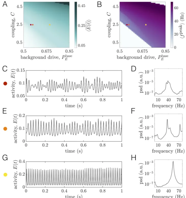
Long-range coupling strength and background drive tune baseline dynamical state.
We begin by computing two measures that quantify regional dynamics:(1) the time-averaged
firing rateEðtÞ, and (2) the frequency at maximum power (peak frequency) fpeakof a given region. To obtain summary measures characterizing the state of the system as a whole, we compute network-averages of these quantities, denoted by angled-brackets. In studying hEðtÞi
as a function ofPbase
E andC, we observe three principal regimes (Fig 2A). When bothP
base
E and
C are low, the system settles to a state of low average firing rate (white region); this state
corre-sponds to a non-oscillatory, low-activity equilibrium. In contrast, whenPbase
E andC are both
high, the average firing rate saturates at a high level (dark green region); this state corresponds to a non-oscillatory, high-activity equilibrium. Finally, at intermediate values of these parame-ters, the mean firing rate varies between the low and high extremes, and the regional activity is oscillatory; because we wish to consider the rhythmic nature of brain activity, this is the rele-vant portion of parameter space.
Next we seek to understand how hfpeaki varies in thePbase
E —C plane (Fig 2B). A clear
wedge-shaped area marks parameter combinations that give rise to network-averaged peak frequen-cies in the gamma range. As with the firing rate, the peak frequency tends to increase
(decrease) with either increasing (decreasing) background excitation or coupling strength. By comparingFig 2B to 2A, we see that the white areas surrounding the purple wedge correspond to the regions of parameter space where the firing saturates at a fixed low or high value. In Sec. SII ofS1 Text, we describe a systematic method for determining boundaries in the 2D space spanned byC and Pbase
E that indicate the onset or disappearance of oscillatory activity (see
Fig. B inS1 Text). In what follows, we useP�
EðCÞ to denote the level of background drive at
which oscillations begin to emerge for a fixed coupling strengthC. We refer the reader to Sec.
SII ofS1 Textfor a detailed description of how this value is determined from the simulations. Furthermore, we often plot quantities as functions of the relative drivePbase
E P � EðCÞ, such that Pbase E P �
EðCÞ ¼ 0 indicates the transition point from a low-activity state to an oscillatory state
at a couplingC.
To provide further intuition for how dynamics vary within this parameter space, we study example time-series and power spectra for three different baseline states (colored dots inFig 2A and 2B). Note that these working points correspond to an intermediate coupling value of
C = 2.5, but varying levels of the constant baseline input Pbase
E . We begin with the working
pointPbase
E ¼ 0:553, which sits just beyond the boundary indicating the transition to sustained
rhythmic activity. From the time-series, we observe that the activity is oscillating (Fig 2C), and the spectra indicates a peak frequency of �40Hz on a broadband background (Fig 2D). We next consider the working pointPbase
E ¼ 0:57. In this state, each unit receives slightly more
drive, leading to higher-amplitude oscillations (Fig 2E and 2F). However, although peak spec-tral power increases, amplitude modulations can still be seen in the corresponding time-series (Fig 2E). Finally, we consider the working pointPbase
Fig 2. Long-range coupling strengthC and background drive Pbase
E modulate firing rates and oscillation frequencies at baseline.(A) The time- and network-averaged population firing rate hEðtÞi as a function of C and Pbase
E (units are arbitrary).(B) The network-averaged peak frequency of regional
activity hfpeaki as a function of
C and Pbase
E .(C) A segment of the activity of one brain area and (D) the corresponding power spectra of the same area at
the working point denoted by the red dot in panelsA and B (Pbase
E ¼ 0:553,C = 2.5). (E) A segment of the activity of one brain area and (F) the
corresponding power spectra of the same area at the working point denoted by the orange dot in panelsA and B (Pbase
E ¼ 0:57,C = 2.5). (G) A segment
of the activity of one brain area and(H) the corresponding power spectra of the same area at the working point denoted by the yellow dot in panels A
andB (Pbase
E ¼ 0:7,C = 2.5).
by regular, high-amplitude oscillations (Fig 2G). Furthermore, inspection of the power spectra indicates a single, narrow peak at a slightly higher frequency than the previous working point (Fig 2H).
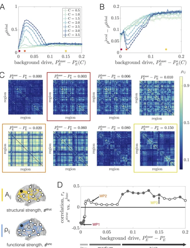
Global phase-coherence is non-monotonically modulated by coupling strength and background drive. Both the firing rate and the power spectra are measures that quantify the
nature of individual regions’ activity. For networks, it is also imperative to define measures that capture information about the extent of dynamical order in the system as a whole. Indeed, for networks of coupled units, the system’s “state” is defined not only by the behavior of indi-vidual units, but also by how their dynamics are interrelated. Here, we are interested in the degree to which regional dynamics are coherent, which we quantify via the PLV between regions’ activities. To compute PLVs for baseline conditions, we begin by filtering the activity of each unit in the same, common frequency band. This band is determined by first finding the peak frequency of each unit at the given working point. Hence, we obtain a set ofN values
ffipeakg corresponding to the peak frequencies of all unitsi2 {1, . . ., N} at baseline. We then
fil-ter the activity of every region in a frequency band spanning 10Hz above the maximum peak frequency in the network (max ffipeakg) and 10Hz below the minimum peak frequency in the
network (min ffipeakg). After identically filtering each unit’s activity in this common band, we
extract Hilbert phases from the filtered signals. Finally, PLVs between all pairs of brain areas are computed according toEq 5, using 50 different simulations (trials) of 5 seconds each (with noise included).
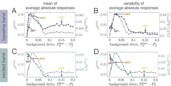
To summarize how the overall level of coherence in the network varies as a function of the background drive and coupling strength, we defined a macroscopic order parameter as the average of the PLVs over all pairs of units in the network:ρglobal= hρiji. This quantity ranges
between 0 and 1, where larger values indicate a more dynamically ordered state of the network. In general, we find that the background input and the coupling strength interdependently tune the level of coherence in the system (Fig 3A). At low coupling, brain areas cannot coordi-nate their dynamics andρglobalremains at a relatively low value for a range of drives. In con-trast, as the coupling is increased, we begin to see a qualitative change in behavior. For higher values ofC, we observe that ρglobalvaries non-monotonically (first increasing and then decreas-ing) as a function of the (relative) background drive. For a given couplingC, there appears to
be a “critical” value at relatively small but non-zeroPbase
E P
�
EðCÞ where the system develops
a well-defined peak in global coherence. As the drive is increased further,ρglobalbegins to decrease and then eventually plateaus, albeit with some fluctuations. More specifically, at levels of background drive well beyond the state of peak coherence,ρglobalrelaxes to an intermediate value between its peak and its value at the lowest background input. In this regime, the system resides in a state of partial order. Increasing the coupling has the effect of amplifying the maxi-mum value ofρglobal(althoughρglobalremains well below 1 for all couplings considered), but does not appear to significantly affect the order parameter to the right side of the peak.
To provide further intuition for this behavior, we focus on an intermediate coupling of
C = 2.5 and examine the pairwise coherence patterns ρijfor several values of the background
drive (Fig 3C). At the lowest (relative) baseline input (Pbase
E P
�
EðCÞ ¼ 0), some organization can
be seen in the PLV matrix, but the system is weakly coherent overall. In this state, units exhibit relatively low amplitude oscillations, and are therefore more influenced by noise. It is thus rea-sonable to expect little phase-locking at low background drive. However, with only a small increase in the non-specific input (e.g.,Pbase
E P
�
EðCÞ ¼ 0:003), we observe distributed increases
in coherence and a large spread of high, medium, and low coherence pairs dispersed throughout the network. Increasing the background drive slightly more (e.g.,Pbase
E P
�
EðCÞ ¼ 0:02) leads to
Fig 3. Long-range coupling strengthC and background drive Pbase
E modulate network phase-coherence and relationships between
structural and functional connectivity at baseline.(A) The global order parameter ρglobalvs. Pbase
E P
�
EðCÞ, for different fixed values of C.
Error bars are estimated from 100 bootstrap samples of the simulations at each coupling and background drive, and correspond to± one standard deviation of the bootstrap disribution ofρglobal.(B) The difference between the global and local order parameters, ρglobal− ρlocal,vs. Pbase
E P
�
near the peak ofρglobaland represents a highly ordered state of the system. As the background drive is increased further, though, phase-locking begins to decrease widely throughout the network and the coherence pattern markedly changes into a more segregated architecture. In particular, for highPbase
E P
�
EðCÞ, we observe the emergence of smaller phase-locked clusters
(Fig 3C, Row 3). To understand this shift in behavior, it is important to note that increasing
Pbase
E increases the extent to which regional activity is independently generated in each areavs.
driven by long-range network interactions. The strengthening of regional oscillations and enhanced influence of local dynamics with increasingPbase
E seems to eventually hinder the ability
of units to adjust their rhythms and achieve widespread coherence. Note that phase-locking is also made especially difficult by the large variance in the distribution of interareal delays imposed by the connectome’s spatial embedding, and indeed, for high background drive conditions, more strongly connected and spatially nearby units are those able to maintain stronger coherence.
In general, our observations point to complex behavior in which the macroscopic order parameter varies non-monotonically as a function of the baseline input and network coupling strength (Fig 3A and 3C). Therefore, a variety of qualitatively different regimes exist, beyond just a simple binary separation into a disordered and ordered state. To more quantitatively dis-tinguish network states before and after the point of peak coherence, we also considered a local order parameter rlocal¼P
ijAijrij=
P
ijAij, which is a weighted average ofρijwith weights equal
to the strength of structural network connections. In this way,ρlocalwill be larger when more strongly connected brain areas are more phase-locked. InFig 3B, we showρlocal− ρglobalvs. Pbase
E P
�
EðCÞ for different values of the coupling C. Beyond a certain point, the curves for all
couplings exhibit a clear upward trend where the extent of local coherence increases relative to the extent of global coherence. This behavior indicates that the macroscopic state of the system becomes increasingly constrained by structure as the background drive increases. Hence, even though the level of global coherence can be similar to the left and right of peakρglobal, the sys-tem is in qualitatively different dynamical modes in the two regimes. Also note that for the higher couplings,ρlocal− ρglobalfirst decreases before consistently rising. This variation occurs because, for large enough coupling strengths, the level of global coherence is able to compete with the level of local coherence at background drives near peakρglobal.
As a final demonstration of the complexity of the structure-function landscape across oper-ating points, we consider the relationship between brain areas’ structural and functional con-nectivity strengths as a function ofPbase
E P
�
EðCÞ for a fixed coupling C = 2.5 (Fig 3D). The
structural strength of nodej, sstruc
j ¼
PN
i¼1Aij, is a common measure of a brain area’s
impor-tance in an anatomical network [98]. Similarly, the (baseline) functional strength of nodej, sfunc
j ¼
PN
i¼1rij, quantifies how dynamically integrated that region is to the network as a whole.
FromFig 3D, we observe that shifting the system’s working point can drastically alter how— and the extent to which—structural strength and functional strength are related. Specifically, while there tends to be a weak positive correlation betweensstrucandsfuncat high background drives (e.g. at WP3), the correlation disappears (e.g. at WP2) and then reverses in sign (e.g. at WP1) as the background drive is lowered. Critically, these transitions occur in the absence of
background drive, and correspond to± one standard deviation of the bootstrap distribution of ρglobal
− ρlocal.
(C) Region-by-region PLV
matrices for various values ofPbase
E P
�
EðCÞ at fixed C = 2.5. The boxed matrices correspond to the red, orange, and yellow working points in
Fig 2and in panels A and B of this figure.(D) The Spearman correlation rsbetween structural node strengthsstrucand functional node
strengthsfunc
vs. Pbase
E P
�
Eat fixedC = 2.5. Empty circles indicate that the correlation was not statistically significant at the p = 0.05 level. The
arrows mark three different working points—WP1, WP2, and WP3 (which correspond to the red, orange, and yellow dots/boxes in this figure)—that will be studied in detail.
any change to the anatomical connectome, and are instead driven by a global change in the behavior of brain areas’ dynamics (induced by changing the level of background input). Also note that when the correlations are significant, they are intermediately-valued. Together, these results indicate that while a given structural network may only be able to support specific pat-terns of coordinated activity, the relationships between the two are not trivial and are modu-lated by dynamic properties [99,100]. In general, functional connectivity thus reflects a complex interplay between both anatomical connectivity and the system’s dynamical state.
It is crucial to remark that the behaviors seen here are more diverse than what tends to occur in simpler phase-oscillator models, where coupling strength is the main control parame-ter and typically induces a monotonic increase in synchrony. A critical difference between phase-based models and the more realistic WC model considered here is that, for the latter case, unit dynamics are described and coupled by real-valued signals that represent regional activity. Hence, widespread changes in the amplitude or stability of areas’ dynamics (in addi-tion to changes in coupling strength) can affect the macroscopic state of the network. Indeed, the preceding analyses show that global modulations in the level of diffuse, constant input to the neural populations can push the system into very different oscillatory modes, beyond just a steady progression from an incoherent to a coherent state. In what follows, we will exploit this behavior to examine how the effects of focal perturbations depend not only on which region is targeted, but also on the baseline working point of brain network dynamics as a whole.
Effects of regional perturbations on brain network activity and dependence
on dynamical state
To investigate how local perturbations modulate brain network dynamics, and specifically how the effects may depend on the system’s collective state, we begin with an in-depth exami-nation of three distinct working points. In particular, we focus on a fixed intermediate cou-pling strengthC = 2.5 for which the system exhibits a clear peak in ρglobal(Fig 3A). We then examine two values of the background drivePbase
E that place the system either in a state
preced-ing (WP1) or followpreced-ing (WP3) the global coherence peak. In Sec. SIII ofS1 Text, we also pres-ent results for a state in which the system is approximately at peak global coherence (WP2). We then proceed to more generally characterize the global impacts of stimulation as the back-ground drive is varied across a wide range. Throughout the text, stimulation of a single brain areai is introduced by increasing its excitatory input by an amount ΔPE,i= 0.1, while keeping
all other regions at their working-point-specific baseline drive. Finally, inS1 Text, we verify that results hold for different values ofPbase
E in the vicinity of those studied in the main text
(Sec. SVIII), we examine the effects of varying the perturbation strength (Sec. SX), and we con-sider an alternative value of the global coupling (Sec. SXI). Note that our goal is not to exhaus-tively analyze all possible parameter combinations, but rather to demonstrate that the network response to stimulation qualititatively varies for different dynamical regimes.
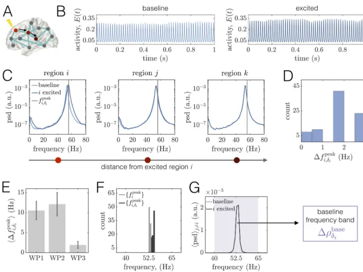
Working point 1: Pre-global coherence peak
We begin with the working point WP1 located atC = 2.5 and Pbase
E P
�
EðCÞ ¼ 0:003, below
peak coherence (Fig 3C, Row 1, Column 2). Here, the system is perched just past the boundary marking the transition between the quiescent state and the commencement of rhythmic dynamics. Hence, regional activity is oscillatory but of relatively low amplitude (seeFig 2C), and the power spectra is broad (seeFig 2D).
Local excitations induce distinct modifications to power spectra. We first examine the
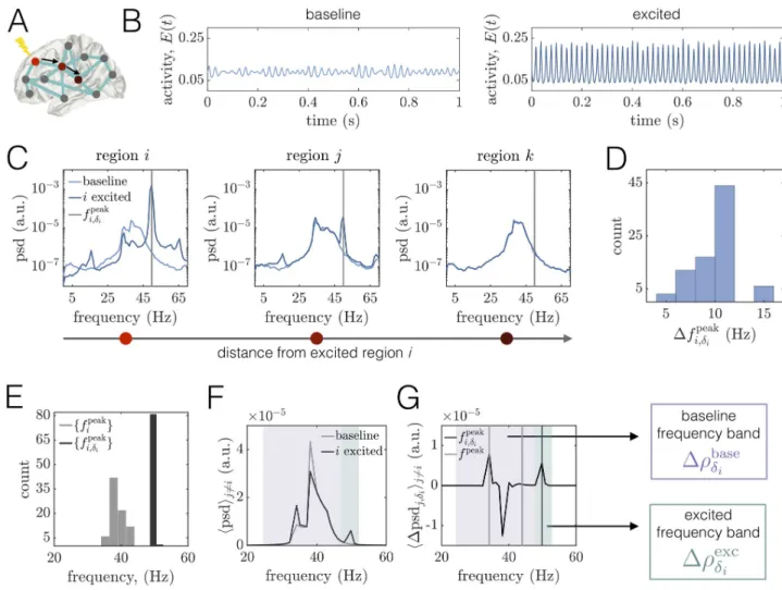
effects of a regional perturbation on areas’ time series and power spectra (Fig 4A–4C). In agreement with past experimental and modeling studies [16,89,101,102], increased drive to
the excitatory pool of regioni increases the amplitude and frequency of its oscillations (Fig 4C, Left). In particular, stimulation causes an increase in the power, narrowing of the spectra (associated with an increase in periodicity of regional activity), and a shift of the peak fre-quency from � 40Hz at baseline to � 50Hz when excited. We also note the appearance of modulation sidebands in the excited spectra to the left and right of the peak frequency, which arise due to the modulation of the excited region’s time-series by the lower-frequency input it
Fig 4. Regional excitation causes local and downstream changes to brain areas’ power spectra in different frequency bands at WP1.(A) Schematic
of a brain network depicting the stimulated sitei in brightest red. The black arrows point to two other regions j and k that lie at progressively further
topological distances from the perturbed area in the structural network. In this figure, regionsi, j, and k correspond to brain areas 1 (R–Lateral
Orbitofrontal), 4 (R–Medial Orbitofrontal), and 10 (R–Precentral), respectively.(B) Left: A segment of region i’s activity time-course in the baseline
condition. Right: A segment of regioni’s activity time-course when it is stimulated. (C) Power spectra of area i and two other downstream regions j and k. In all three panels, the lighter curves correspond to the baseline condition, and the darker curves correspond to the state in which i is driven with
additional input. The gray vertical lines indicate the peak frequencyfpeak
i;di of regioni in the excited condition. (D) Histogram of the shift in peak
frequency Dfpeak
i;di induced by stimulating uniti, plotted over all choices of the perturbed area. (E) Distribution of peak frequencies of all units in the
baseline condition ffpeak
i g (light gray) and distribution of the peak frequency units acquire when directly excited ff peak
i;di g (dark gray).(F) Average power
spectra hpsdij6¼iover all unitsj 6¼ i at baseline (light gray) and when unit i is perturbed with additional input (dark gray). (G) Average difference
hDpsdj;diij6¼iof the spectra of unitj 6¼ i when unit i is excited and in the baseline condition, where the average is over all units j 6¼ i. For reference, the
light gray vertical lines denote the minimum and maximum peak frequency across units in the baseline state, and the dark gray line indicates the peak frequency acquired by the stimulated regioni. Shaded boxes denote two frequency bands of interest: (1) the baseline band (purple) consisting of the
main oscillation frequencies of brain areas under baseline conditions, and(2) the excited band (green) centered around the peak frequency that the
stimulated region inherits. In subsequent analyses, we assess perturbation-induced changes in the PLV between brain areas in the baseline band, Drbase di
(purple), and in the excited band Drexc di (green). https://doi.org/10.1371/journal.pcbi.1008144.g004
receives from other areas in the network [92]. This modulation also results in a spectral peak at � 16Hz—which is the difference between the new, excited frequency and the sideband peaks, and is a marker of quasiperiodic amplitude modulation in the time-series. To more carefully quantify the effects of an excitation to regioni, we consider the shift in the peak frequency of
uniti, Dfi;dpeaki ¼f
peak
i;di f
peak
i , between its excited and baseline states (Fig 4D). Calculating these
differences for all choices of the stimulated brain area, we find that they range from about 6Hz to 16Hz, with an average value of hDfi;dpeaki i � 10:5 Hz. These perturbation-induced shifts thus
yield excited peak frequencies that are well-separated from the range of peak frequencies in the baseline state (Fig 4E).
We next consider the power spectra of two other unitsj and k located at increasing
topolog-ical distances from the excited region, where a shorter topologtopolog-ical distance indicates that two areas are linked by a path of stronger structural connections [98]. (Fig 4C, Middle, Right). We observe that unitj maintains its initial frequency content, but also develops new peaks centered
at the frequency of the excited region and at the difference of the excited frequency and the baseline peak. In contrast, the spectra of unitk—which is more weakly structurally connected
to the stimulated site—is relatively unchanged. Hence, depending on the network structure, stimulation of regioni can also cause alterations to other regions’ spectra. In general, the
power modulation of a downstream area’s spectra at the peak frequency of the stimulated site decays with increasing topological distance between the dowstream area and the perturbed region (see Sec. SV inS1 Text). To summarize how the spectra of other brain areas are altered by driving regioni with additional input, we compare the average power spectral density
hpsdij6¼iover all unitsj 6¼ i at baseline and when unit i is stimulated (Fig 4F). At baseline, the
network-averaged spectra is relatively broad and contains multiple peaks—a main one at 38Hz and a smaller peak around 34Hz. In addition, a local excitation produces complex and broad-band alterations in power, as expected in a scenario of quasiperiodic entrainment between nonlinear oscillators [103]. For this example, we observe the appearance of an entirely new peak at 50Hz, but also an enhancement of the lowest baseline peak and a depression of the highest baseline peak. These changes are perhaps more apparent inFig 4G, which shows the average difference hDpsdj;d
iij6¼iin the spectra of unitj 6¼ i between when unit i is excited and
the baseline condition, where the average is over all unitsj 6¼ i. In sum, we see that a regional
enhancement of neural activity causes non-local modulations in power both at the frequency of the directly stimulated brain area, as well as at the system’s baseline oscillation frequencies. These analyses suggest that there are two relevant frequency bands to consider for subsequent analysis:(1) a relatively broad band containing the main frequencies of brain areas in the
base-line state, and(2) a band centered around the peak frequency of the excited unit. In what
fol-lows, we will denote these two bands as “baseline” and “excited”, and consider changes in phase-locking, Drbase
di and Dr exc
di , in each band induced by local perturbations.
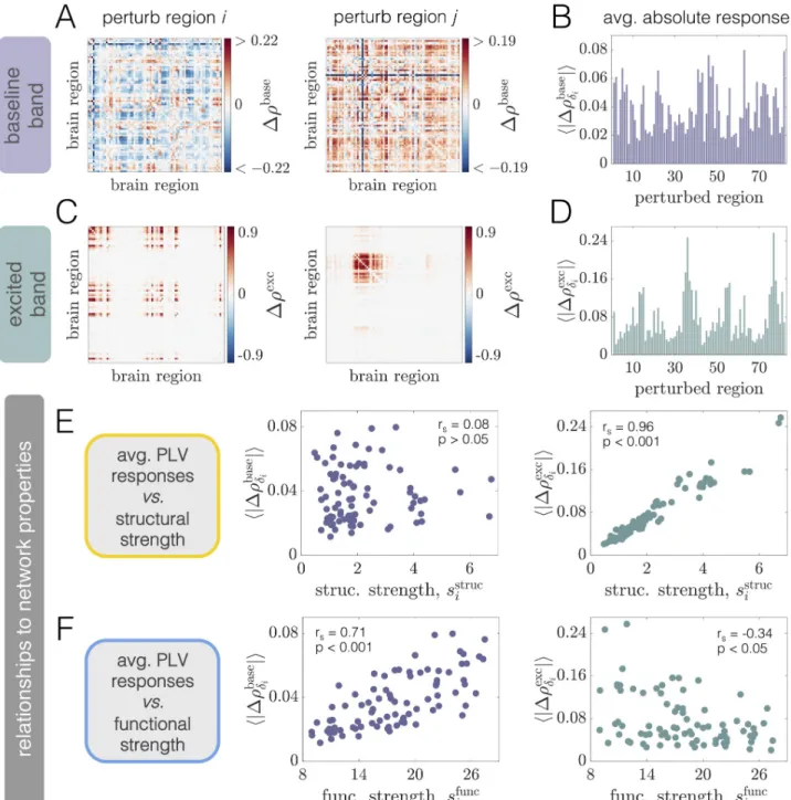
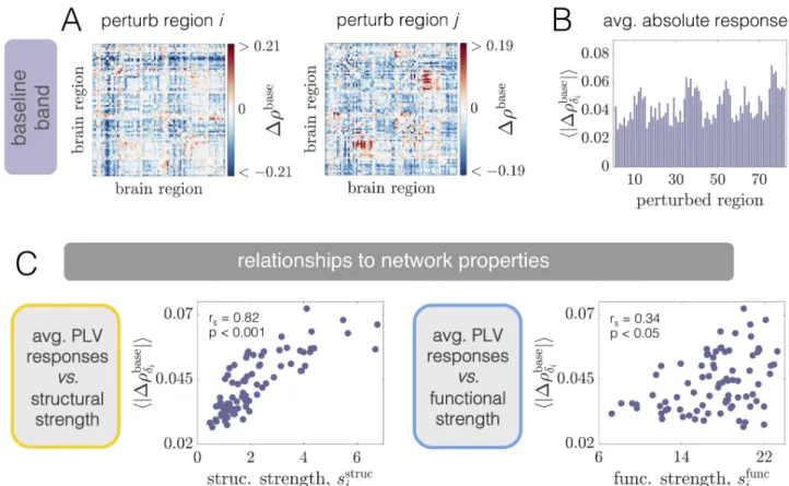
Excitations of regional activity induce or alter interareal phase-locking in excited and baseline frequency bands. We are now prepared to study how focal perturbations alter the
coordination of network-wide dynamics. Specifically, we examine changes in interareal phase-locking. We separate our analysis into two frequency bands—baseline and excited—by filter-ing regional activity in each band, extractfilter-ing Hilbert phases from the filtered signals, and then calculating the PLV for each pair of regions within each band (seeFig 1E;Materials and methods). Since spectra are relatively broad at baseline, a single baseline frequency band for the network is determined by first finding the set of peak frequencies for each uniti in the
baseline state, ffipeakg. Next, the lower frequency for the common baseline band is set to
min ffipeakg 10 Hz, and the upper frequency is set tomax ff
peak