HAL Id: hal-01351209
https://hal.archives-ouvertes.fr/hal-01351209
Submitted on 2 Aug 2016
HAL is a multi-disciplinary open access
archive for the deposit and dissemination of
sci-entific research documents, whether they are
pub-lished or not. The documents may come from
teaching and research institutions in France or
abroad, or from public or private research centers.
L’archive ouverte pluridisciplinaire HAL, est
destinée au dépôt et à la diffusion de documents
scientifiques de niveau recherche, publiés ou non,
émanant des établissements d’enseignement et de
recherche français ou étrangers, des laboratoires
publics ou privés.
Joint Analysis of Multiple Datasets by Cross-Cumulant
Tensor (Block) Diagonalization
Dana Lahat, Christian Jutten
To cite this version:
Dana Lahat, Christian Jutten. Joint Analysis of Multiple Datasets by Cross-Cumulant Tensor (Block)
Diagonalization. SAM 2016 - 9th IEEE Sensor Array and Multichannel Signal Processing Workshop,
Jul 2016, Rio de Janeiro, Brazil. �hal-01351209�
JOINT ANALYSIS OF MULTIPLE DATASETS
BY CROSS-CUMULANT TENSOR (BLOCK) DIAGONALIZATION
†Dana Lahat and Christian Jutten
GIPSA-Lab, UMR CNRS 5216, Grenoble Campus, BP46, 38402 Saint-Martin-d’H`eres, France
ABSTRACT
In this paper, we propose approximate diagonalization of a cross-cumulant tensor as a means to achieve independent component anal-ysis (ICA) in several linked datasets. This approach generalizes ex-isting cumulant-based independent vector analysis (IVA). It leads to uniqueness, identifiability and resilience to noise that exceed those in the literature, in certain scenarios. The proposed method can achieve blind identification of underdetermined mixtures when single-dataset cumulant-based methods that use the same order of statistics fall short. In addition, it is possible to analyse more than two datasets in a single tensor factorization. The proposed approach readily extends to independent subspace analysis (ISA), by tensor block-diagonalization. The proposed approach can be used as-is or as an ingredient in various data fusion frameworks, using coupled decompositions. The core idea can be used to generalize existing ICA methods from one dataset to an ensemble.
Index Terms— Independent vector analysis; tensor diagonal-ization; blind source separation; coupled decompositions; data fu-sion
1. INTRODUCTION
In this paper, we propose a cumulant-based approach for the joint analysis of an ensemble of datasets that admit the independent vec-tor analysis (IVA) [1] model. IVA is a framework that addresses an ensemble of independent component analysis (ICA) [2] problems by exploiting not only the statistical independence within each dataset but also dependence among latent sources in different datasets. IVA is further explained in Section 2. An advantage of IVA over analysing each dataset individually is that it aligns the estimated sources in all datasets with the same (arbitrary) permutation, thus obviating the need to resolve the individual arbitrary permutation in each mixture separately. In addition, IVA can generally separate mixtures of Gaussian real stationary sources with spectra identical up to a scaling factor, a problem that does not have a unique solu-tion when each mixture is treated individually. In this paper, we add to the list of useful properties of IVA (i) better resilience to certain types of noise, and (ii) enhanced uniqueness and identifiability in the presence of underdetermined mixtures, for non-Gaussian data.
Most IVA-type methods use cross-correlations, i.e., second-order cross-cumulants, e.g., [3–6], or a multivariate contrast with a nonlinear function, e.g., [1, 7]. The idea to explicitly use cross-cumulants of higher-order statistics (HOS) for IVA first appeared in [8, 9]. Their idea is to jointly diagonalize slices of cross-cumulant tensors, where each cross-cumulant involves a pair of datasets. In
This work is supported by the project CHESS, 2012-ERC-AdG-320684. GIPSA-Lab is a partner of the LabEx PERSYVAL-Lab (ANR–11-LABX-0025).
†This is very close to the official version, published in Proc. SAM 2016.
order to jointly process several sets of (cross) cumulants, the factor-izations are coupled in a specific way that was termed generalized joint diagonalization (GJD). IVA via GJD can be applied to second-order statistics (SOS) and up. When fourth-second-order statistics are used, GJD can be regarded as a multiset counterpart of joint approximate diagonalisation of eigen-matrices (JADE) [10]. The GJD analyti-cal framework in [9] is prewhitening-based and not designed to deal with underdetermined scenarios. When introducing GJD, Li et al. [9] mention that in principle, one may use cross-cumulants taken from more than two datasets. However, they proceed only with pairs of cross-cumulants, explaining that groups of more than two contribute less to the separation than slices involving variables from only two datasets, due to noise and finite sample size. In this paper, we ex-plain, in Section 2, how cross-cumulants that involve K ≥ 2 differ-ent datasets can achieve enhanced resilience to noise. We show how methods based on cross-cumulants enjoy uniqueness and identifia-bility that exceed those of single-dataset cumulant-based methods that use the same order of statistics. Finally, our approach allows to analyse more than two datasets in a single tensor factorization, as opposed to GJD. For SOS, i.e., K = 2, GJD coincides with our approach. For K ≥ 3, our approach is, naturally, not suitable for Gaussian data.
In the following, we denote scalars, vectors, matrices and higher-order arrays (tensors) by a, a, A and A, respectively. The nth column and (m, n)th entry of A are denoted by anand am,n,
respectively. (·)>and k · k denote transpose and the Frobenius norm, respectively. The mode-n product ×nbetween C ∈ RI1×···×INand
A ∈ RJn×In yields an I
1 × · · · × In−1× Jn× In+1· · · × IN
array whose entries are given by [C ×nA]i1,...,in−1,jn,in+1,...,iN =
PIn
in=1ci1,...,in,...,iNajn,in[11, Definition 4]. The outer product of
N non-zero vectors an∈ RIn×1is a rank-1 I1×· · ·×INtensor C =
a1◦ · · · ◦ aNwhose entries are given by ci1,...,iN = a1,i1· · · aN,iN.
2. MODEL AND PROBLEM FORMULATION Consider K datasets, each admitting an ICA model,
x[k](t) = A[k]s[k](t) + n[k](t) 1 ≤ t ≤ T , 1 ≤ k ≤ K (1) where A[k] ∈ KI[k]×R
, x[k](t) ∈ KI[k]×1and s[k](t) ∈ KR×1 represent a mixing matrix, observations and latent sources, respec-tively, whose elements are real or complex, K ∈ {C, R}. The ele-ments of s[k](t) are sampled from random vectors that follow the IVA model. IVA is a generalization of ICA to multiple datasets in which the K elements of random vector sr = [s
[1] r , . . . , s
[K] r ]>,
r = 1, . . . , R, are statistically dependent whereas the pairs (sr, sr0)
are statistically independent for any r 6= r0. The noise random pro-cesses n[k]∈ KI[k]×1
are mutually statistically independent for any k 6= k0, as well as statistically independent of all sources.
A[1] A[2]
A[3]
cum(s[1], s[2], s[3])
cum(x[1], x[2], x[3])
Fig. 1: Diagonalization of a third-order cross-cumulant tensor. In this example, K = 3 and R = 4.
Given a set of observations X = {x[k](t)}Kk=1,t=1,T , the goal of IVA is to separate the sources and/or identify the mixtures by exploit-ing not only the statistical independence within each set of measure-ments but also the dependence among sets of measuremeasure-ments. When-ever A[k]is full column rank, the corresponding samples s[k](t) may
be estimated by multiplying x[k](t) with a left inverse of an estimate of A[k]. Otherwise, the samples cannot be estimated without resort-ing to additional assumptions (e.g., [12, Chapter 9.2.1]). The latter often occurs when I[k]< R, i.e., underdetermined. In this case, one has to suffice with “blind identification”, i.e., estimating only A[k]. In this paper, we propose to achieve these inferences by factorizing a cross-cumulant tensor, as we now explain.
For K ≥ 2, the Kth-order I[1]× · · · × I[K]
cross-cumulant of X is given by CK X = cum(x [1] , . . . , x[K]) = CKS ×1A[1]×2A[2]× · · · ×KA[K] (2)
(holds for K = 1 if the noise has zero mean) where the Kth-order R × · · · × R cross-cumulant CK
S = cum(s[1], . . . , s[K]) is
diag-onal. A key assumption is that the main-diagonal elements do not vanish. The right-hand side (RHS) of (2) is due to the linearity prop-erty of cumulants (e.g., [13, Chapter 2]). The noise term vanishes from the cross-cumulants, even for K = 2, due to its statistical in-dependence properties. We conclude that approximating a sample cross-cumulant of X with the model in (2) yields estimates of all factors A = {A[k]}K
k=1, with the added benefit of (asymptotically)
getting rid of the noise at no additional computational cost. Figure 1 illustrates this idea.
2.1. Implications
Equation (2) can be rewritten as CK X= R X r=1 cKsra [1] r ◦ a[2]r ◦ · · · ◦ a[K]r (3)
where cKsr denotes the Kth-order cumulant of s
[1]
r , . . . , s[K]r , cKsr =
cum(s[1]r , . . . , s[K]r ). Equation (3) rewrites CKXas a sum of R
rank-1 terms, where the rth summand represents the contribution of the rth source in all K datasets. For the smallest R for which (3) holds exactly, this factorization amounts to canonical polyadic decompo-sition (CPD) [14, 15]/parallel factor analysis (PARAFAC) [16]. This fact has the following implications.
Uniqueness: CPD is generically unique under mild conditions (e.g., [17, 18]). Hence, the proposed approach is naturally suitable for underdetermined ICA. Furthermore, the ensemble may admit a unique decomposition even if some of the underdetermined ICA are not identifiable individually with the same order of statistics. We point out that the cumulant-based GJD framework has a simi-lar uniqueness property. The idea that coupled decompositions can provide uniqueness of the ensemble even when each dataset is not individually unique has already been proved in certain types of cou-pled tensor decompositions [19] and SOS-based IVA [20]. Hence, the proposed approach is another demonstration of the enhanced uniqueness capacities of coupled decompositions.
Computation: Basically, we may optimize (2) and (3) with any general-purpose algorithm that approximates a Kth-order ten-sor with a sum of R rank-1 terms. A similar observation has previ-ously been made with respect to (w.r.t.) underdetermined ICA [12, Chapter 9.4.3]. For a discussion of various aspects of CPD opti-mization for source separation, see, e.g., [12, Chapter 9.4.3] and ref-erences therein. Dedicated tensor diagonalization algorithms such as [21–23] may also be used, whenever the data admits their model assumptions. Constraints such as orthogonality may be imposed as well, e.g., [24]. Since (2) amounts to a Tucker [25] format with a diagonal core, then, in principle, one may use any general-purpose Tucker decomposition algorithm for the optimization. However, uniqueness issues inherent to Tucker-type decompositions may re-sult in difficulty attributing factors to specific sources and hence, weaker interpretability.
2.2. Generalization to Multidimensional Components
Until now, we discussed only ICA and rank-1 components. How-ever, all previous results are readily generalizable to rank-L[k]r ≥ 1
(this variant of IVA is sometimes termed joint independent sub-space analysis (JISA) [26, 27]) by replacing the diagonal structure of the tensor with block-diagonal. For example, in the third-order case in Figure 1, the rth block on the diagonal now stands for an L[1]r × L[2]r × L[3]r cube instead of a 1 × 1 × 1 scalar. The
correspond-ing factorization is “decomposition in rank-(L[1]r , L[2]r , . . . , L[K]r )
terms” [28]. Apart from the block term decomposition (BTD) al-gorithms in, e.g., [29, 30], it has been proposed to use tensor diago-nalization to uncover the underlying block structure [22, 23].
A concluding remark is in order. Whereas ICA has numerous cumulant-based methods, with independent subspace analysis (ISA) the situation is quite different. The first cumulant-based approach to ISA is [31], which proposes to “partially diagonalize” a fourth-order cumulant tensor. A subspace variant of JADE is proposed in [32]. Tichavsk´y et al. [22] mention that tensor block-diagonalization can be applied to cumulant-based ISA; however, they do not develop further this idea.
3. NUMERICAL VALIDATION
In this section, we illustrate by numerical examples the capability of the proposed approach to separate sources and identify mixtures in well-posed and underdetermined scenarios.
3.1. Figure of Merit
Whenever A[k]has full column rank, we are interested in the quality
of separation of x[k](t) = PR r=1x
[k]
r (t) into R unique rank-1
obser-vations using x[k]r (t) = P[k]r x[k](t), where the rank-1 I[k]×I[k]
ma-trices P[k]r are oblique projections onto span(a [k]
r ) orthogonally to
all span(a[k]r0), r
0
6= r, and can be computed directly from A[k]
[33]. Similarly,bx[k]r (t) = bP
[k]
r x[k](t), via bA[k], for their estimated
coun-terparts. We choose to quantify the quality of separation using the normalized empirical mean square error (MSE)
[ MSE[k]r = T X t=1 kxb [k] r (t) − x [k] r (t)k 2 / T X t=1 kx[k]r (t)k 2 (4)
The use of scale-invariant projections obviates the need to normalize the source samples in order to find an optimal match with the original samples, in the performance analysis stage. Another motivation is that scale-invariant projections are the natural way to deal with terms of rank larger than one [33], see Section 2.2; scale-dependent objects require normalization, which is not well-defined.
In the underdetermined case, when the sources cannot be sepa-rated, we quantify the quality of blind identification, i.e., estimation of each factor A[k], using the relative error, defined as
RelErr[k]=kA
[k]− bA[k]k
kA[k]k (5)
In order to correct the arbitrary permutation and scaling within each estimate bA[k]
, we use Tensorlab [30]’s function cpderr. 3.2. Experimental Setup
We compare our approach with two cumulant-based algorithms, JADE [10] and GJD [9], both are prewhitening-based. We test our proposed cross-cumulant diagonalization approach in two scenarios. In the first, the factors are unconstrained. In the second, full col-umn rank factors are constrained to be orthogonal (there is no added value in orthogonality in underdetermined mixtures [34]). Both sce-narios were implemented using CPD-based algorithms, which were applied to the same whitened samples as the other algorithms. This experimental setup allows us to compare the prewhitening-based al-gorithms, as well as obtain some further insights about the potential of the CPD for this task.
In order to compute the normalized empirical MSE (4) we first have to align the estimated components w.r.t. their true values. As explained in Section 1, for GJD and our proposed approach, only the arbitrary permutation of the R rank-1 elements needs to be found. For JADE, however, we must find this permutation individually for each dataset. A wrong permutation results in significantly higher MSE. In the following examples, since only K = 4 datasets are involved, we detect this permutation by simple enumeration on all 4 or 4! combinations and picking up the best.
Since JADE uses fourth-order cumulants, our experimental setup involves K = 4 datasets. Each dataset consists of R = 3 sources and T = 2 · 103 sampling points. The entries of A[k] are drawn independently from the standard normal distribution. We generate non-Gaussian samples that follow the IVA model by defin-ing, for each r, two unit-variance independent symmetric Gaussian mixture (GM) processes with peaks centred at ±4/√17, and then combining them using α[k]r ∼ U [0, 1], which is drawn
indepen-dently at each sample: s[k]r = α [k]
r g1,r + (1 − α [k]
r )g2,r, where
g1,r, g2,r ∼ GM. The resulting overall random process is
nor-malized to unit variance. In the following numerical experiments, A[k]are drawn once and kept fixed throughout M C = 200 Monte Carlo (MC) trials, in which source samples are drawn anew. We
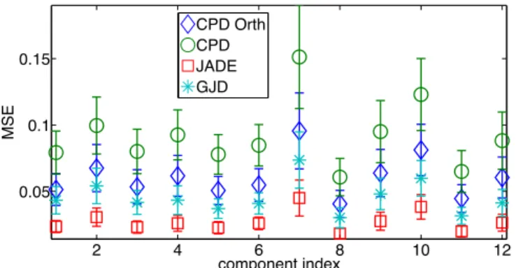
2 4 6 8 10 12 0.05 0.1 0.15 component index MSE CPD Orth CPD JADE GJD
Fig. 2: Normalized MSE in ICA of K = 4 datasets using fourth-order statistics. In each dataset, A[k] ∈ R3×3
and R = 3 sources. Error bars denote empirical standard deviation. The MSE of compo-nent x[k]r is given at component index [r + (k − 1)R].
do not apply additive noise, so estimation error is only due to fi-nite sample size. For JADE and GJD, we use online-available code1 with options “N2” and “whole” for GJD. For CPD, we use a Ten-sorlab [30] implementation with TolFun= 10−12, TolX= 10−12. The unconstrained CPD is optimized using cpd_nls, where, for each MC trial, we take the best out of 25 random initializations. CPD with orthogonal factors is optimized using sdf_minf via struct_orth, where the factors are initialized with random val-ues (only once per trial).
1st experiment: Source separation in invertible mixtures. In a first step, we validate proper functionality of our proposed ap-proach in a basic setup of invertible A[k] ∈ RR×R ∀k. Figure 2
depicts the normalized empirical MSE in the estimation of each com-ponent. For each pair (k, r), we removed trials for which at least one type of algorithm did not achieve separation2. In this experiment,
two trials, which corresponds to component #7 in Figure 2, were removed due to large error in unconstrained CPD.
2nd experiment: blind identification. In a second step, we present the capability of the proposed method to achieve blind identification of underdetermined mixtures. Consider the case of A[k]
∈ R2×3
, k = 1, 2, 3. By straightforward counting of de-grees of freedom, one can verify that ICA with R = 3 sources and I[k]= 2 detectors is generally not unique and not identifiable if one exploits only statistics up to order four and all data is in the real domain (e.g., [35, 36]). With our approach, however, this is possi-ble. We guarantee the uniqueness of the CPD of our fourth-order cross-cumulant tensor by setting A[4]∈ R3×3[18]. Hence, this
ex-periment consists of three underdetermined ICA that cannot be iden-tified by any fourth-order method and one ICA that can be solved by ordinary JADE3. The GJD algorithm [9] is not suitable for datasets
with underdetermined mixtures and is thus excluded from this exper-iment. JADE can be applied only to the fourth dataset. The relative error (5) for all K = 4 factors using CPD is depicted in Figure 3. The normalized empirical MSE in the estimation of all rank-1 com-ponents in the 4th dataset using JADE and CPD is given in Figure 4.
1http://perso.telecom-paristech.fr/∼cardoso/Algo/Jade/jadeR.m,
http://mlsp.umbc.edu/codes/jbss cum4.m
2With certain draws of A[k], both orthogonal and unconstrained CPD did
often not converge to a desired solution, regardless of initialization. This matter deserves to be further looked into. For the examples in this paper, only data with no estimation issues were selected.
3In fact, stronger uniqueness is generally possible. For example, there
are enough degrees of freedom already at two underdetermined mixtures and fourth-order statistics. In addition, a mixing matrix that can be estimated individually may be regarded as a known factor in the ensemble.
0.50 1 1.5 2 2.5 3 3.5 4 4.5 0.02 0.04 0.06 0.08 0.1 0.12 factor index k Relative error CPD Orth CPD
Fig. 3: Relative error in estimating A[k] in K = 4 datasets, each
with R = 3 sources. A[k=1,2,3]∈ R2×3
. A[4]∈ R3×3
. Error bars denote empirical standard deviation.
0.5 1 1.5 2 2.5 3 3.5 0 0.05 0.1 0.15 0.2 0.25
component index r in 4th dataset
MSE
CPD Orth CPD JADE
Fig. 4: Normalized MSE in ICA of K = 4 datasets, each with R = 3 sources. A[k=1,2,3] ∈ R2×3
. A[4] ∈ R3×3
. Here, we depict the MSE only for k = 4.
3.3. Discussion of Numerical Results
The small values of MSE and relative error in Figures 2, 3 and 4 imply successful separation and blind identification. JADE is the al-gorithm that makes an overall most efficient use of the fourth-order statistics within each dataset and indeed, it achieves the best MSE. The fact that GJD performs worse than JADE deserves to be further looked into. We point out that [8, 9] did not compare with JADE. Orthogonally-constrained CPD consistently performs better than the unconstrained CPD, and pretty close to GJD. Given that CPD uses less statistical information than GJD, this is an encouraging indica-tion to the usefulness of the proposed approach. The rather poor performance of unconstrained CPD cannot be explained just by the difference between non-orthogonal vs. prewhitening-based methods. In fact, when testing unconstrained CPD on non-prewhitened sam-ples, its performance was even worse. A possible explanation may be the larger number of variables to estimate in unconstrained fac-tors, compared with fewer ones when orthogonality is imposed. In addition, the cost function of CPD is different than directly mini-mizing off-diagonal values, a matter than may be more significant in large sample perturbation. Other algorithms (Section 2.1) may per-form better. Therefore, although unconstrained CPD achieves the smallest residual error in estimating the original cumulant tensor, it may not be the best candidate for our approach compared with other tensor diagonalization methods. This matter deserves to be further looked into. The fact that orthogonality constraints are void in the
underdetermined scenario explains why the relative error is similar for both types of CPD in the first three factors in Figure 3. The performance of the proposed approach may be enhanced by cou-pling with SOS [10, Sec. 4.2] or with other (cross-) cumulants that carry complementary information. It is interesting to observe where the trade-off between different types of combinations of statistics is, both in terms of error and in computational cost.
The overall conclusion from these experiments is that our paradigm is correct, and that our cross-cumulant tensor diagonal-ization approach indeed successfully exploits statistical links among datasets to achieve blind identification of underdetermined mixtures even in “adverse” scenarios, when the order of statistics is limited and individual ICA is impossible. However, for more conclusive statements about the usefulness of our proposed approach w.r.t. state of the art, these preliminary numerical results serve only as a proof of concept, and require further theoretical and experimental support.
4. CONCLUSION
In this paper, we have shown that factorizing a cross-cumulant ten-sor of several datasets can achieve simultaneous ICA of all in-volved mixtures, if certain conditions hold. We explained how cumulant-based IVA may achieve uniqueness of the ensemble that exceeds that of individual underlying datasets, extending previous results on SOS-IVA. We have shown analytically that using cross-cumulants provides, asymptotically, resilience to dataset-specific noise. The proposed approach relies directly on the strong unique-ness of CPD/BTD. Even stronger uniqueunique-ness, identifiability and in-terpretability may be achieved by coupling several arrays, adding types of diversity (e.g., nonstationarity), various assumptions and constraints within and among datasets. The proposed approach mo-tivates multiset variants of tensor-based ICA methods such as JADE, its higher-order generalizations [37, 38], or methods based on the characteristic function [39] to use this cross-cumulant concept to achieve stronger uniqueness.
5. REFERENCES
[1] T. Kim, T. Eltoft, and T.-W. Lee, “Independent vector analy-sis: An extension of ICA to multivariate components,” in In-dependent Component Analysis and Blind Signal Separation, ser. LNCS, vol. 3889. Springer Berlin Heidelberg, 2006, pp. 165–172.
[2] P. Comon, “Independent component analysis,” in Proc. Int. Signal Process. Workshop on HOS, Chamrousse, France, Jul. 1991, pp. 111–120,
[3] H. Hotelling, “Relations between two sets of variates,” Biometrika, vol. 28, no. 3/4, pp. 321–377, Dec. 1936. [4] J. Kettenring, “Canonical analysis of several sets of variables,”
Biometrika, vol. 58, no. 3, pp. 433–451, 1971.
[5] Y.-O. Li, T. Adalı, W. Wang, and V. D. Calhoun, “Joint blind source separation by multiset canonical correlation analysis,” IEEE Trans. Signal Process., vol. 57, no. 10, pp. 3918–3929, Oct. 2009.
[6] M. Anderson, T. Adalı, and X.-L. Li, “Joint blind source sep-aration with multivariate Gaussian model: Algorithms and performance analysis,” IEEE Trans. Signal Process., vol. 60, no. 4, pp. 1672–1683, Apr. 2012.
[7] M. Anderson, G.-S. Fu, R. Phlypo, and T. Adalı, “Indepen-dent vector analysis, the Kotz distribution, and performance
bounds,” in Proc. ICASSP, Vancouver, Canada, May 2013, pp. 3243–3247.
[8] X.-L. Li, M. Anderson, and T. Adalı, “Second and higher-order correlation analysis of multiple multidimensional variables by joint diagonalization,” in Latent Variable Analysis and Signal Separation, ser. LNCS, vol. 6365. Heidelberg: Springer, 2010, pp. 197–204.
[9] X.-L. Li, T. Adalı, and M. Anderson, “Joint blind source sep-aration by generalized joint diagonalization of cumulant ma-trices,” Signal Process., vol. 91, no. 10, pp. 2314–2322, Oct. 2011.
[10] J.-F. Cardoso and A. Souloumiac, “Blind beamforming for non-Gaussian signals,” Radar and Signal Process., IEE Pro-ceedings F, vol. 140, no. 6, pp. 362–370, Dec. 1993.
[11] L. De Lathauwer, B. De Moor, and J. Vandewalle, “Blind source separation by higher-order singular value decomposi-tion,” in Proc. EUSIPCO, vol. 1, Edinburgh, Scotland, UK, Sep. 13–16 1994, pp. 175–178.
[12] P. Comon and C. Jutten, Eds., Handbook of Blind Source Sep-aration: Independent Component Analysis and Applications, 1st ed. Academic Press, Feb. 2010.
[13] D. R. Brillinger, Time Series, Data Analysis and Theory. San Francisco, CA: Holden-Day, 1981.
[14] F. L. Hitchcock, “The expression of a tensor or a polyadic as a sum of products,” J. Math. Phys., vol. 6, no. 1, pp. 164–189, 1927.
[15] J. D. Carroll and J.-J. Chang, “Analysis of individual differ-ences in multidimensional scaling via an N -way generalization of “Eckart-Young” decomposition,” Psychometrika, vol. 35, no. 3, pp. 283–319, Sep. 1970.
[16] R. A. Harshman, “Foundations of the PARAFAC procedure: models and conditions for an “explanatory” multimodal factor analysis,” UCLA Working Papers in Phonetics, vol. 16, pp. 1– 84, Dec. 1970.
[17] J. B. Kruskal, “Three-way arrays: rank and uniqueness of tri-linear decompositions, with application to arithmetic complex-ity and statistics,” Linear Algebra Appl., vol. 18, no. 2, pp. 95–138, 1977.
[18] N. D. Sidiropoulos and R. Bro, “On the uniqueness of multilin-ear decomposition of N -way arrays,” J. Chemometrics, vol. 14, no. 3, pp. 229–239, May–Jun. 2000.
[19] M. Sørensen and L. De Lathauwer, “Coupled canonical polyadic decompositions and (coupled) decompositions in multilinear rank-(Lr,n, Lr,n, 1) terms—part I: Uniqueness,”
SIAM J. Matrix Anal. Appl., vol. 36, no. 2, pp. 496–522, Apr. 2015.
[20] J. V´ıa, M. Anderson, X.-L. Li, and T. Adalı, “Joint blind source separation from second-order statistics: Necessary and sufficient identifiability conditions,” in Proc. ICASSP, Prague, Czech Republic, May 2011, pp. 2520–2523.
[21] M. Sørensen, P. Comon, S. Icart, and L. Deneire, “Approxi-mate tensor diagonalization by invertible transforms,” in Proc. EUSIPCO, Glasgow, Scotland, UK, Aug. 2009, pp. 500–504. [22] P. Tichavsk´y, A. H. Phan, and A. Cichocki, “Non-orthogonal
tensor diagonalization, a tool for block tensor decompositions,” arXiv:1402.1673 [cs.NA], 2015.
[23] Y. Liu, X.-F. Gong, and Q. Lin, “Non-orthogonal tensor diag-onalization based on successive rotations and LU decomposi-tion,” in Proc. ICNC, Zhangjiajie, China, Aug. 2015, pp. 102– 107.
[24] M. Sørensen, L. De Lathauwer, P. Comon, S. Icart, and L. Deneire, “Canonical polyadic decomposition with a colum-nwise orthonormal factor matrix,” SIAM J. Matrix Anal. Appl., vol. 33, no. 4, pp. 1190–1213, 2012.
[25] L. R. Tucker, Contributions to Mathematical Psychology. New York: Holt, Rinehardt & Winston, 1964, ch. The exten-sion of factor analysis to three-dimenexten-sional matrices, pp. 109– 127.
[26] D. Lahat and C. Jutten, “Joint independent subspace analy-sis using second-order statistics,” IEEE Trans. Signal Process., vol. 64, no. 18, pp. 4891–4904, Sep. 2016.
[27] R. F. Silva, S. Plis, T. Adalı, and V. D. Calhoun, “Mul-tidataset independent subspace analysis extends independent vector analysis,” in Proc. ICIP, Paris, France, Oct. 2014, pp. 2864–2868.
[28] L. De Lathauwer, “Decompositions of a higher-order tensor in block terms. Part II: Definitions and uniqueness,” SIAM J. Matrix Anal. Appl., vol. 30, no. 3, pp. 1033–1066, 2008. [29] L. De Lathauwer and D. Nion, “Decompositions of a
higher-order tensor in block terms. Part III: Alternating least squares algorithms,” SIAM J. Matrix Anal. Appl., vol. 30, no. 3, pp. 1067–1083, 2008.
[30] L. Sorber, M. Van Barel, and L. De Lathauwer, “Tensorlab v2.0,” Jan. 2014. [Online]. Available: http://www.tensorlab. net/
[31] L. De Lathauwer, B. De Moor, and J. Vandewalle, “Fetal elec-trocardiogram extraction by source subspace separation,” in Proc. IEEE SP/ATHOS Workshop on HOS, Girona, Spain, Jun. 1995, pp. 134–138.
[32] F. J. Theis, “Towards a general independent subspace analysis,” in Proc. NIPS, 2007, pp. 1361–1368.
[33] J.-F. Cardoso, “Multidimensional independent component analysis,” in Proc. ICASSP, vol. 4, Seattle, WA, May 1998, pp. 1941–1944.
[34] L. De Lathauwer, “Simultaneous matrix diagonalization: the overcomplete case,” in Proc. ICA, vol. 8122, Nara, Japan, Apr. 2003, pp. 821–825.
[35] P. Comon, “Tensor diagonalization, a useful tool in signal pro-cessing,” in Proc. IFAC-SYSID, vol. 1, Copenhagen, Denmark, Jul. 1994, pp. 77–82.
[36] L. De Lathauwer, P. Comon, B. De Moor, and J. Vandewalle, “ICA algorithms for 3 sources and 2 sensors,” in Proc. IEEE Sig. Process. Workshop on HOS, Caesarea, Israel, Jun. 1999, pp. 116–120.
[37] L. De Lathauwer, B. De Moor, and J. Vandewalle, “Indepen-dent component analysis and (simultaneous) third-order tensor diagonalization,” IEEE Trans. Signal Process., vol. 49, no. 10, pp. 2262–2271, 2001.
[38] E. Moreau, “A generalization of joint-diagonalization criteria for source separation,” IEEE Trans. Signal Process., vol. 49, no. 3, pp. 530–541, Mar 2001.
[39] P. Comon and M. Rajih, “Blind identification of under-determined mixtures based on the characteristic function,” Sig-nal Process., vol. 86, no. 9, pp. 2271–2281, Sep. 2006, special Section: Signal Processing in UWB Communications.

![Fig. 3: Relative error in estimating A [k] in K = 4 datasets, each with R = 3 sources](https://thumb-eu.123doks.com/thumbv2/123doknet/14225851.484599/5.918.82.450.106.304/fig-relative-error-estimating-k-datasets-r-sources.webp)
