Constraining the Neutron Star Mass-Radius Relation and
Dense Matter Equation of State with NICER. II. Emission
from Hot Spots on a Rapidly Rotating Neutron Star
The MIT Faculty has made this article openly available.
Please share
how this access benefits you. Your story matters.
Citation
Bogdanov, Slavko et al. “Constraining the Neutron Star
Mass-Radius Relation and Dense Matter Equation of State with NICER.
II. Emission from Hot Spots on a Rapidly Rotating Neutron Star”
Astrophysical Journal Letters, vol. 887, no. 1, 2019, L26 © 2019 The
Author(s)
As Published
https://dx.doi.org/10.3847/2041-8213/ab5968
Publisher
American Astronomical Society
Version
Final published version
Citable link
https://hdl.handle.net/1721.1/125720
Terms of Use
Article is made available in accordance with the publisher's
policy and may be subject to US copyright law. Please refer to the
publisher's site for terms of use.
Constraining the Neutron Star Mass
–Radius Relation and Dense Matter Equation of
State with
NICER. II. Emission from Hot Spots on a Rapidly Rotating Neutron Star
Slavko Bogdanov1 , Frederick K. Lamb2,3 , Simin Mahmoodifar4 , M. Coleman Miller5 , Sharon M. Morsink6 , Thomas E. Riley7 , Tod E. Strohmayer4 , Albert K. Tung6, Anna L. Watts7 , Alexander J. Dittmann5, Deepto Chakrabarty8 ,
Sebastien Guillot9,10 , Zaven Arzoumanian11, and Keith C. Gendreau11
1
Columbia Astrophysics Laboratory, Columbia University, 550 West 120th Street, New York, NY 10027, USA;slavko@astro.columbia.edu
2
Center for Theoretical Astrophysics and Department of Physics, University of Illinois at Urbana-Champaign, 1110 West Green Street, Urbana, IL 61801-3080, USA 3
Department of Astronomy, University of Illinois at Urbana-Champaign, 1002 West Green Street, Urbana, IL 61801-3074, USA 4
Astrophysics Science Division and Joint Space-Science Institute, NASA Goddard Space Flight Center, Greenbelt, MD 20771, USA 5
Department of Astronomy and Joint Space-Science Institute, University of Maryland, College Park, MD 20742-2421, USA 6
Department of Physics, University of Alberta, Edmonton, AB T6G 2G7, Canada 7
Anton Pannekoek Institute for Astronomy, University of Amsterdam, Science Park 904, 1090GE Amsterdam, The Netherlands 8
MIT Kavli Institute for Astrophysics and Space Research, Massachusetts Institute of Technology, 70 Vassar Street, Cambridge, MA 02139, USA 9
IRAP, CNRS, 9 avenue du Colonel Roche, BP 44346, F-31028 Toulouse Cedex 4, France 10
Université de Toulouse, CNES, UPS-OMP, F-31028 Toulouse, France 11
X-Ray Astrophysics Laboratory, NASA Goddard Space Flight Center, Greenbelt, MD 20771, USA Received 2019 September 24; revised 2019 November 10; accepted 2019 November 13; published 2019 December 12
Abstract
We describe the model of surface emission from a rapidly rotating neutron star that is applied to Neutron Star Interior Composition Explorer X-ray data of millisecond pulsars in order to statistically constrain the neutron star mass–radius relation and dense matter equation of state. To ensure that the associated calculations are both accurate and precise, we conduct an extensive suite of verification tests between our numerical codes for both the Schwarzschild + Doppler and Oblate Schwarzschild approximations, and compare both approximations against exact numerical calculations. We find superb agreement between the code outputs, as well as in comparisons against a set of analytical and semi-analytical calculations, which, combined with their speed, demonstrates that the codes are well suited for large-scale statistical sampling applications. A set of verified, high-precision reference synthetic pulse profiles is provided to the community to facilitate testing of other independently developed codes. Unified Astronomy Thesaurus concepts:High energy astrophysics(739);Neutron stars(1108);Gravitation(661); Pulsars(1306);Millisecond pulsars(1062);Rotation powered pulsars(1408);Special relativity(1551);General relativity(641)
Supporting material: tar.gzfile
1. Introduction
If a spinning neutron star (NS) radiates X-rays from one or more hotter regions(hereafter “hot spots”) on or near its surface and the gas in these spots rotates with the star at a regular rate, a distant observer will see periodic, energy-dependent pulsations. It is widely recognized that the observed pulsations offer a valuable probe of the physical conditions and processes occurring at or very near the neutron star surface. Statistical estimates of the gravitational mass M and the circumferential radius R of several NSs with sufficiently different masses are of particular interest: they can provide crucial information about the formation and evolution of NSs, and can be used to constrain the properties of the cold, dense interior matter(see, e.g., Özel et al.2016; Steiner et al.2016; Baillot d’Etivaux et al.2019). The stellar properties M and R can be jointly estimated byfitting models to the observed X-ray pulsations, because the properties of the observed pulsed signal are affected by both parameters. The characteristics (or absence) of occultations of the hotter regions as the star rotates constrain the stellar radius. The observed morphology of the pulsations depends on M via general relativistic light deflection, which increases with increasing stellar compactness M/R. For discussions of the various approximations that have been used to compute these effects, see Pechenick et al. (1983), Strohmayer (1992), Miller & Lamb (1998), Braje et al. (2000), Beloborodov (2002), Poutanen & Gierliński (2003), Cadeau et al. (2007),
Morsink et al. (2007), Psaltis & Özel (2014), and Nättilä & Pihajoki(2018).
The line-of-sight velocity of the X-ray emitting gas, and hence the relativistic Doppler boost and aberration it produces, is proportional to the product of the stellar radius and the spin rate. Hence, other things being equal, the changes in the pulse profile produced by these effects are larger for stars that are spinning more rapidly. Consequently, waveformfitting usually provides the strongest constraints on R and M when it is used to analyze the pulse profiles produced by NSs with millisecond spin periods. NSs that produce X-ray flux oscillations with millisecond periods include accretion-powered millisecond X-ray pulsars (see Poutanen & Gierliński 2003; Poutanen & Beloborodov2006; Leahy et al.2008,2009,2011; Morsink & Leahy2011; Salmi et al.2018afor recent models, and Patruno & Watts2012for a description of the observations); NSs that produce thermonuclear X-ray bursts that have millisecond brightness oscillations (see Strohmayer et al. 1997; Miller & Lamb1998; Weinberg et al. 2001; Bhattacharyya et al. 2005; Artigue et al.2013; Lo et al.2013; Psaltis et al.2014; Bauböck et al.2015; Miller & Lamb2015for pulse profile models, and Watts2012for a discussion of the observations), and rotation-powered millisecond pulsars that appear to have hotter regions near their magnetic polar caps that produce periodic X-ray brightness modulations(see Braje et al.2000; Bogdanov et al. 2007,2008; Bogdanov 2013for the models).
The observed pulse profile depends on M and R in various ways, both in the combination of the compactness ratio M/R and separately. It follows that these parameters can in principle be measured individually by carefully analyzing the waveform of the X-ray emission from the star. Providing such measure-ments is one of the principal goals of NASA’s Neutron Star Interior Composition Explorer(NICER) mission (see Gendreau et al. 2016), which was launched and installed on the International Space Station in 2017 June. Thefirst crucial step in assuring the correctness of such an analysis is to verify that the model pulse profiles being used are computed correctly for the assumed properties of the star, the assumed properties of its emission, and the direction and distance to the observer. This Letter documents our procedures for performing such calculations.
The purpose of this Letter is (i) to describe the model we apply to energy-resolved X-ray pulsations of millisecond pulsars observed by NICER to obtain constraints on their M– R relation, (ii) present the results of a series of tests that we have devised to ensure that our algorithms and codes produce precise and accurate results, (iii) offer clarifications and corrections to the procedures commonly used to model the surface emission from rapidly rotating neutron stars, and (iv) provide a set of verified high-precision synthetic pulse profiles for those who wish to verify their own calculations.
This Letter is the second in a series of papers dedicated to obtaining new information about the NS M and R and the dense matter equation of state (EoS) using data of several nearby millisecond pulsars obtained with NICER. In Bogdanov et al. (2019, hereafter Paper I), we present the data collected so far for target MSPs that are being analyzed for this purpose. Bogdanov et al.(2019, hereafter PaperIII) describes all other aspects of the modeling technique applied to the NICER data, including neutron star atmospheres, interstellar absorption, the instrument response, and the M and R parameter estimation methodology, and the potential sources of systematic error. The first set of results for PSR J0030+0451 of the parameter estimation analyses that are based in part on the model described here are presented in Miller et al. (2019) and Riley et al.(2019).
This Letter is organized as follows. In Section2we describe the essential ingredients of the Schwarzschild + Doppler (S+D) approximation, while in Section3we explore the next-order Oblate Schwarzschild(OS) approximation (Cadeau et al. 2007; Morsink et al. 2007). In Sections 4 and 5 we give the results from the comparison tests that have been performed on the S+D and OS approximations, respectively, between our codes as well as against exact general relativistic numerical calculations. In the appendices, we give examples of analytic or semi-analytic calculations that agree with the results of our codes and we present descriptions of the codes used in the verification.
2. Modeling Hot Spot Emission from NSs in the S+D Approximation
A rotating NS is not perfectly spherical and the spacetime external to the star is not exactly Schwarzschild. If we wished to compute the waveforms from rotating hot spots with the greatest possible accuracy and precision, we would therefore have to solve the exact general relativistic equations for the stellar shape and exterior spacetime metric using an
axisymmetric code such as RNS(Stergioulas & Friedman1995) or LORENE/NROTSTAR (Vincent et al.2018) and then trace the rays in that spacetime. Numerical relativistic ray tracing using the metric corresponding to a rapidly rotating NS with a tabulated EoS was first performed by Cadeau et al. (2007). Their procedure involvedfirst choosing an EoS, and computing the equations of relativistic stellar structure using the RNS code for a choice of mass and spin. This results in a solution for the non-spherical shape of the rotating star and the metric for the star evaluated on a spatial grid. This calculation takes on the order of tens of seconds to compute on a modern processor. Once the metric has been computed, an initial latitude on the star’s surface is chosen, and geodesics emitted from this location are emitted in all directions allowed by the star’s surface. Once the geodesics connecting an initial and final angular location are found for all values of phase, a pulse waveform can be constructed. On a modern processor, this procedure takes on the order of many tens of minutes to construct a pulse profile. Alternate codes (Nättilä & Pihajoki 2018; Pihajoki et al.2018; Vincent et al.2018) that can do the same problem with similar accuracy and speed have been developed more recently.
The analysis of NICER data requires the generation of up to hundreds of millions of synthetic pulse waveforms. Thus, speed as well as accuracy is essential. With that in mind, the first approximation that we make is the S+D approximation (see Miller & Lamb 1998; Nath et al. 2002; Poutanen & Gierliński 2003; Strohmayer 2004; Lo et al. 2013). In this approximation, all special relativistic effects at the stellar surface are treated correctly but the star is approximated as a sphere and the spacetime external to the star is assumed to be the Schwarzschild spacetime. Cadeau et al.(2007) showed that their more general treatment of geodesics on the correct numerical spacetime reduces to the S+D approximation in the slow rotation limit. This approximation is extremely fast and is useful for slowly rotating stars(for rotation frequencies ν that are less than ≈100 Hz), as we expect that observational data will have statistical errors larger than the waveform differences introduced by the rotational deformation of the metric and the surface. The more accurate OS approximation, appropriate for more rapidly spinning pulsars, will be investigated in more detail in the following section.
We begin in Section 2.1 with a discussion of emission of light from a spot on a non-gravitating uniformly rotating sphere in the context of special relativity in order to point out an error in a number of previous publications when the surface area is defined in the comoving frame. This is followed in Section2.2 with the addition of gravity to the rotating sphere. Because in what follows we make use of a large number of variables, with symbols that are not consistently used in the literature, for convenience we provide Figure1and Table5in the Appendix summarizing the notation used here.
2.1. Emission from the Surface of a Uniformly Rotating Non-gravitating Sphere
Consider the emission of light from a non-gravitating sphere that has a radius R as measured in a local static frame and rotates uniformly with an angular frequencyΩ as seen in that frame. We wish to compute the energy-resolvedflux seen by a distant observer from a spot that rotates with the sphere on its surface. The observer is at a distance D from the star, far
enough away that the light rays originating from the sphere are parallel to each other. There is no gravity, so light rays are straight lines. The considerations that we discuss will also apply to oblate stars, but the spherical case is easier to picture.
2.1.1. Emission from an Infinitesimal Patch on the Surface of the Sphere
Suppose that we are interested in an infinitesimal patch of the emitting star, which has a linear extent that corresponds to a range of colatitudes between θ and θ+dθ, and to a range of azimuths between f and f+df. The star rotates in the +f direction as seen by static observers. The solid angle is a Lorentz invariant, which means that both a local comoving observer riding on the patch and a local static observer directly above the patch will measure the solid angle of the patch to be sin q q fd d .
However, as is shown in various references (e.g., the excellent pedagogical discussion in Kassner 2012), although the linear extent of the patch in theθ direction,Rdq, is the same in the comoving and the static frames, the linear extent of the patch in thef direction, which is measured to be R sin q fd by a static observer directly above the patch, is measured to be
( )
g q R sinq fd by the comoving observer, where
( ) [ ( )] ( )
g q º 1 -b q2 -1 2 1
is the Lorentz factor corresponding to the dimensionless speed
( ) ( )
b q º WRsinq c 2
seen by a static observer at colatitude θ. Thus a spot that appears to be circular when measured in linear coordinates in the comoving frame will appear to be compressed in the direction of motion to a local static observer, while a star that appears spherical to local static observers will appear oblate to local comoving observers. This effect, derived purely in special relativity, also needs to be included(with modifications to the definition of the velocity) in a treatment with gravity. Some
previous publications(e.g., Miller & Lamb1998; Poutanen & Gierliński2003; Bogdanov et al.2007; Leahy et al.2008) used an incorrect expression for the comoving surface element, which neglected the factor γ(θ). This error was discussed by Psaltis et al.(2016), Lo et al. (2018), and Nättilä & Pihajoki (2018). The codes used for the parameter estimation analyses presented in Miller et al. (2019) and Riley et al. (2019) correctly include thisγ(θ) factor.
Suppose now that we are interested in a light ray emerging from the star that makes an angleξ with the local direction of motion, as seen in the static frame. Then, the Doppler factor
( )[ ( ) ] ( ) d g q b q x º -1 1 cos 3
can be used to convert the values of several useful quantities from the comoving frame to the static frame. Using the convention that primed quantities are measured in a local inertial frame that is momentarily comoving with the stellar surface (hereafter referred to as the local comoving frame), whereas unprimed quantities are measured in the local static frame, the angles from the local surface normal are related by ( )
a=d- a¢
cos 1cos , 4
photon energies are related by
( )
d
= ¢
E E , 5
and specific intensities are related by
( a)=d ¢ ¢( a¢) ( )
I E, 3I E, . 6
An observer at a distance D?R from the star will therefore measure theflux from an infinitesimal patch on the star that is centered at(θ′, f′)=(θ, f) to be ( ) ( ) ( ) ( ) a q f a q f a d a q f a = = ¢ ¢ ¢ ¢ ¢ ¢ ¢ dF E I E dS D I E dS D , , , , , , cos , , , cos , 7 2 3 2
where the surface area element in the local comoving frame is defined by
( ) ( ) ( )
g q q q f g q q q f
¢ = ¢ ¢ ¢ ¢ =
dS R2sin d d R2sin d d . 8
The light travel time from the patch to the observer depends on the location of the patch at the time of emission. One way to take this into account is to first compute the non-rotating azimuthal radiation pattern that would be seen at the inclination and distance of the observer, taking into account exactly all the special relativistic effects on the energy, beaming, etc., of the radiation that is produced by the star’s rotation. Once this time-independent radiation pattern has been computed as a function of photon energy, the pattern can be rotated at the stellar spin frequency to obtain the observed time-dependent waveform.
Using this approach, the time-dependentflux at an observer located at(ζ, fobs) and f(t)=Ωt can be written
(z f )= (z f( )) ( )
dFobs , obs,t dF0 , t . 9
In this approach, it is the time dependence of the argumentf(t) that produces the time dependence of the observed flux
(z f )
dFobs , obs,t . Note that, as measured in the local comoving
frame, the emission from the surface is steady(even variation produced by, e.g., spreading of thermonuclear burning occurs
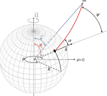
Figure 1.Geometry of a hot spot on the surface of a neutron star rotating at an angular frequencyΩ. A photon emitted from the surface at an angle α with respect to the local surface normal n, as seen in the local static frame, deflects by a total angle ψ as it travels to a distant observer. Figure adapted from Bogdanov(2016).
on timescales that are much longer than typical stellar rotation periods). It is only the non-axisymmetry of the emission combined with rotation that causes the flux seen by a distant observer to vary.
2.1.2. Emission from an Extended Spot on a Rotating Sphere
The flux as a function of time from an extended spot is simply the integral of thefluxes from the infinitesimal patches that make up the spot. Care must be taken to ensure that the photons that are counted in the flux all arrive at the distant observer at the same time. That is, if the times needed to reach the distant observer from two different points of emission on the star differ byΔt, then the difference in the emission times from the two points needs to be−Δt so that both of the rays reach the observer simultaneously.
As a specific example, consider a small spot on the equator of the rotating star, as seen by an equatorial observer. Let f=0 be the point directly underneath the observer. Then, emission from an infinitesimal patch at azimuth f (where −π/2 f π/2 because we assume a very distant observer and light travels on straight-line paths in our special relativistic example) will have a propagation time to the observer that is Δt=(R/c)(1 − cos f) longer than the propagation time of a radial ray. Thus, if the pulse waveform is folded on the angular frequency Ω, the flux from this emission will contribute to a phasefobs=f+ΩΔt rather than to fobs=f.
2.2. Modeling Emission from a Gravitating Star in a Schwarzschild Exterior Spacetime
We now move from consideration of rotating non-gravitating stars to rotating gravitating stars. Nothing about the transfor-mation between local comoving and local static observers will change. However, light will not travel in straight lines, and gravitational redshifts must be taken into account.
A major advantage to using the Schwarzschild spacetime, in contrast to spacetimes that have frame dragging, is that the spherical symmetry of the Schwarzschild geometry guarantees that the path followed by any given photon lies in a plane. Hence, the procedure for tracing the path of a light ray from any angular location(θ, f) on the stellar surface to any angular location(ζ, fobs) at a large distance is simple.
1. Determine the deflection angle y =cos-1[(q f, ) · (z f, obs)] between the starting and ending points of the ray.
2. Determine the angleα from the surface normal, as seen in the local static frame at the stellar surface, such that a photon leaving the surface at that angle will be deflected by an angleψ in propagating to infinity.
3. Using, e.g., spherical triangles (or the great circle distance), determine the local azimuthal angle λ (defined, for example, so that λ = 0 points north and λ = π/2 points east) such that an arc of angular size ψ, in the direction λ, connects (θ, f) at the surface to (ζ, fdist) at infinity.
Thus, no actual tracing of a photon is required: a simple table look-up ofψ(α) suffices to determine the needed direction from the stellar surface. This results in a tremendous saving of computational time.
We show the geometry of the system in Figure 1. We consider an infinitesimal hot spot at a colatitude θcwith respect
to the stellar rotational pole(finite-sized hot spots can be built by linear addition of infinitesimal spots) seen by an observer at a colatitudeζ. If we denote by f(t) the azimuthal angle of the spot as a function of time(where f = 0 means that the spot is at the same longitude as the observer), then the angular distance ψ(t) between the spot and the observer is given by
( ) ( ) ( )
y t = q z f t + q z
cos sin csin cos cos ccos . 10 It is useful to break the computation of the waveform seen by a distant observer into two separate frame shifts: (1)from a surface comoving frame to a local static frame at the surface; and(2)from the local static frame to the distant observer. The first involves only local special relativistic transformations, whereas the second requires non-local general relativistic effects. In both cases, it is helpful to use the constancy of IE/E3along rays, where E is the energy of a photon and IEis the specific intensity at E, to follow the effect of redshifts and blueshifts on the specific intensity. We now discuss the special relativistic effects, followed by the general relativistic effects.
2.2.1. From the Surface Comoving Frame to the Static Frame
It is typically assumed that an observer at the stellar surface who moves with the star will see a particularly simple specific intensity of emission. For example, it is standard to assume that in this frame, the specific intensity depends only on the angle from the local normal and not on the azimuthal angle of emission. For testing purposes, we sometimes assume an isotropic beaming pattern, although such a pattern is not expected for real systems. For example, the non-accreting rotation-powered NSs that are the focus of the NICER mission likely have the beaming patterns of non-magnetic light-element atmospheres (H or He; see Potekhin 2014 and references therein). We use primes to denote quantities measured in the surface comoving frame, e.g.,α′ is the angle from the normal as seen in the comoving frame.
The Lorentz transformation from the surface comoving frame to the frame of a temporarily co-located static observer is local. The speed of the surface as measured by that local static observer is
( ) q ( )
= W -
-v R 1 RS R 1 2sin c, 11
whereW º 2pn is the rotational angular frequency of the star as seen at infinity and RS=2GM/c2 is the Schwarzschild radius. The equations defining the transformation from the surface comoving frame to the local static frame are similar to those given in Section2.1.2, except that the velocity is given by Equation(11), which is corrected for gravitational redshift. The relativistic Doppler factorδ is
[ ( ) ] ( ) d g x = - v c 1 1 cos , 12
whereg =[1-(v c) ]2-1 2 is the Lorentz factor andξ is the
angle of the photon’s propagation relative to the direction of rotation, as seen by a local static observer. The relation between the angleα′ of the photon propagation direction relative to the surface normal in the comoving frame and the angleα relative to the surface normal in the local static frame is
( )
a¢ =d a
Moreover, if the area of the infinitesimal surface patch is dS′ as seen in the comoving frame, then the area of the same patch as seen in the local static frame is
( )
d
= ¢
dS dS , 14
which means thatdScosa=dS¢cosa¢is a Lorentz invariant (Lightman et al. 1975; Lind & Blandford1985).
2.2.2. From the Surface Static Frame to the Distant Observer
Once the transformation has been made to the surface static frame, the propagation of photons to a distant observer introduces several effects.
Gravitational redshift. In the Schwarzschild spacetime, gravitational redshifts depend only on the initial and final radius and not on the direction of propagation. The photon energy seen by an observer at a large distance D is (1- R RS )1 2 times the photon energy seen by an observer in the local static frame at the stellar radius R. The relation between the photon energy E′ emitted in the local comoving frame and the photon energy E measured by the observer far from the star is
( ) ( )
d
= - ¢
E 1 RS R1 2E 15
which appears similar to Equation (5), but includes both the gravitational redshift and the Doppler shift from Equation(3). Light deflection. The relation between ψ and α is (Misner et al.1973; Pechenick et al.1983)
⎜ ⎟ ⎡ ⎣⎢ ⎛ ⎝ ⎞⎠ ⎤ ⎦⎥ ( )
ò
( ) y b R = ¥ dr - - -r b r R r , 1 1 1 16 R S 2 2 2 1 2 where ( ) a = -b R R R 1 S sin 17is the impact parameter of a light ray originating from the neutron star radius R that is emitted at an angleα with respect to the radial direction, as seen in the local static frame.
For sufficiently compact stars (R/Rs 1.76), light-ray bending angles can be>π, resulting in the entire surface being always visible and regions on the NS having multiple photon trajectories that can reach the distant observer(see Ftaclas et al. 1986). The code used for the parameter estimation analyses in Miller et al.(2019) accounts for this possibility. The code used in Riley et al. (2019) does not do so, due to the extra computational complexity required to include multiple images. We note, however, that the favored ranges of M and R for PSRJ0030+0451 from both analyses do not cover the regime of compactness where multiply imaged regions are relevant.
Time delays. Photons with larger deflection angles ψ also travel a larger distance to an observer, which in turn means that their propagation time is longer. The actual time of propagation to infinity is infinite for any ray, but it is convenient to subtract the propagation time of a radial ray(Pechenick et al.1983):
⎜ ⎟ ⎪ ⎪ ⎪ ⎪ ⎧ ⎨ ⎩ ⎡ ⎣⎢ ⎛ ⎝ ⎞⎠ ⎤ ⎦⎥ ⎫ ⎬ ⎭ ( ) ( )
ò
D = -´ - - -¥ -t b R c dr R r b r R r , 1 1 1 1 1 . 18 R S S 2 2 1 2This time delay translates into a phase lag(Δf) of a photon ( )
f
D = WDt, 19
and thus the measured rotational phase is fobs=femit+ Df for a photon emitted at phase femit (Viironen & Poutanen 2004).
The observedflux. When the various factors are combined, the spectralflux from a surface element ¢dS seen by an observer
at distance D is (see, e.g., the derivation in Section 3.1 of Poutanen & Gierliński2003)
( ) ( ) d ( a) a a ( ) y = - ¢ ¢ ¢ ¢ ¢ dF E R R I E d d dS D 1 , cos cos cos , 20 S 1 2 3 2
where the surface area element in the co-rotating frame is given by dS¢ = gR2sinq q fd d , as in the special relativistic case.
The lensing factor d(cosa) d(cosy) accounts for the divergence of nearby light rays as they propagate away from the star, causing an element of area on the star to appear larger to an observer far from the star. The factord(cosa) d(cosy) has the limiting value of(1 − RS/R) for light emitted normal to the surface (α = 0). For values of RS/R<0.568, as α increases,d(cosa) d(cosy)does as well, but the dependence is non-monotonic for more compact stars. The number flux
(
df E) of photons with energy E in the detector is related to the
spectralflux bydf E( )=dF E( ) E.
2.3. Surface Gravity
In Schwarzschild geometry, the acceleration due to gravity on the surface of a spherical star is given by the corrected Newtonian formula(see Zeldovich & Novikov1971)
⎜ ⎟ ⎛ ⎝ ⎞⎠ ( ) = - -g R R GM R 1 S . 21 0 1 2 2
The surface gravity is of importance when using realistic emission models such as NS atmospheres, as the EoS and radiative-transfer properties of the atmosphere are determined in part by this parameter (see, e.g., Heinke et al. 2006, and references therein). As discussed in Section 3, for oblate stars the effective acceleration due to gravity for a given colatitude is expressed relative to g0.
3. Modeling Hot Spot Emission from NSs in the OS Approximation
For stars that are rotating sufficiently rapidly (ν 200 Hz), the rotation-induced oblateness of the stellar surface is significant, and the S+D approximation is inadequate. To address this shortcoming, Morsink et al.(2007) developed the oblate-star Schwarzschild spacetime approximation in which the spacetime of the NS is described by the Schwarzschild metric, the special relativistic Doppler boost and aberration and time delays are implemented in the same manner as in the S+D approximation, but the oblateness of the NS surface is also taken into account. In our current OS models that are applied to NICER data, the spin-dependent shape of the rotating star is incorporated through the use of a convenient formula derived by AlGendy & Morsink(2014):
( )q = [ + ( W¯ ) ( )]q ( )
where Reqis the equatorial circumferential radius of the neutron star, ¯W = W R(2 eq RS)
3 1 2, and the expansion coefficient is
expressed as o2 = W¯ (o +o x)
2
20 21 and is given in Table 1 of
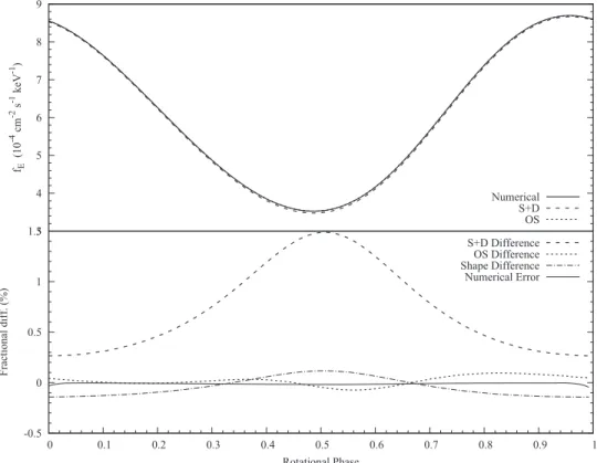
AlGendy & Morsink (2014). AlGendy & Morsink (2014) computed the coefficients on using different libraries of proposed EoS and found that the specific choices of tabulated EoS did not significantly alter the values of the coefficients. It should be noted that the choices for the order of the polynomial fits does introduce small differences in the shape function, as can be seen with comparisons with the earlier shape function introduced by Morsink et al. (2007). In order to quantify the potential errors introduced by the shape function, pulse shapes using the two different shape functions are compared in the lower panel of Figure 2 with the curve denoted “Shape Difference.” This shows that the potential errors introduced by the shape function are at approximately the 0.1% level for the test model that spins at 200 Hz. For stars rotating much more rapidly (say at 600 Hz or higher), it would be advisable to investigate an empirical shape function optimized for rapid rotation.
On an oblate star, the surface area of a small spot of angular sizes dθcand df located at angles θcandf on the surface of the star will have a surface area
( )q = ( )q q[ + ( )]q q f ( )
dS c R2 c sin c 1 f2 c 1 2d dc 23
where the function f(θc) is defined by
( )q ( ) ( ) q = - -f R R R dR d 1 . 24 c S c 1 2
Unlike the spherical case, away from the equator and spin pole, the direction normal to the surface of an oblate star is not generally the radial direction. As a result, it is necessary to consider the photon emission direction σ relative to the local zenith angle,
( ) ( )
s= a t l t + a t
cos sin sin cos cos cos , 25 whereτ is the angle between the radial direction and the local surface normal, given by
[ ( )] ( ) ( )
t= +f q - t=f +f q
cos 1 2 c 1 2 and sin 1 2 c , 26 while spherical trigonometry yields cosl( )t =(cosz
-) ( )
q y q y
cos ccos sin csin . We note that the angleτ is positive for points on the“northern” hemisphere (i.e., the hemisphere closer to the observer), while τ is negative for points in the “southern” hemisphere.
In the OS approximation, the exterior spacetime remains as the Schwarzschild solution, so the deflection of outward rays can be computed using Equation (16), as in the S+D approximation. Because the surface of an oblate spheroid is tilted with respect to a spherical surface, some outward-directed rays will be eclipsed by the oblate surface.
The oblateness of the star requires special treatment of light rays that originate from the surface in radially inward trajectories that would be blocked by the stellar surface if the surface were spherical, but can reach the observer due to surface tilting. These photonsfirst travel to smaller values of r until a critical radial coordinate rcis reached, and then move
Figure 2.Comparison offlux measured at 1keV for the S+D and OS approximations and the exact numerical waveform for one sample star. The example star spins with a frequency of 200 Hz, has M=1.44 Me, Req=11.41 km. The upper panel shows waveforms computed using the S+D and OS approximations, as well as the
outward. The impact parameter of an initially ingoing photon is ( ) ( ) ( ) q q - b R R R 1 , 27 c S c in
for an angleα>π/2. The critical radius is determined by the solution of the equation
( ) = -r b R r 1 . 28 c S c in
The bending angle corresponding to a photon trajectory between R(θc) to rcis given by the integral
⎜ ⎟ ⎡ ⎣ ⎢ ⎛⎝ ⎞⎠⎤ ⎦ ⎥ ( ) ( )
ò
y D = q - -b dr r b r R r 1 1 . 29 r R S in 2 in 2 2 1 2 c cOwing to symmetry, the inward Rrc and outwardrcR
trajectories have the same bending angle, leading to a total bending angle for an initially ingoing photon of
( ) ( ) ( )
yin bin,R = D +2 y y b R, 30 where ψ(b, R) is given by Equation (16). As expected, an initially ingoing photon will have a larger bending angle and take longer to reach the observer than an initially outgoing photon with the same value of impact parameter. If the star were more compact than R=3GM/c2, some inward-directed photons would hit the surface instead of escaping to infinity. However, we have limited R/(GM/c2) to be greater than 3.2, and wefind that for the rotation frequencies we explore, no ray that initially moves away from the surface returns to intersect the surface again.
The flux measured by an observer at a distance D from a surface element on an oblate star is
( ) ( ) ( ) ( ) d s s a y = - ¢ ¢ ¢ ´ ¢ ¶ ¶ ¢ dF E R R I E dS D 1 , cos cos cos , 31 S R 1 2 3 2
where the area element in the co-rotating frame is, similar to the spherical case, the Lorentz γ factor times Equation (23).
3.1. Photon Propagation Time Delays
The treatment of travel time delays in the OS approximation is similar to the S+D case, but requires additional corrections. One correction arises from the fact that, relative to a photon emitted from the stellar equator, photons at other colatitudes have to travel out toward the observer starting from a smaller radius. Additionally, because photons are emitted from different depths in the gravitational potential of the star (with photons at the spin poles having to climb out further compared to equatorial photons), they will experience different levels of time dilation. Defining a radial photon emitted from the stellar equator as a reference, the total time delays for photons emitted from an oblate star as a function of colatitude can be
expressed as ⎜ ⎟ ⎪ ⎪ ⎪ ⎪ ⎧ ⎨ ⎩ ⎡ ⎣⎢ ⎛ ⎝ ⎞⎠ ⎤ ⎦⎥ ⎫ ⎬ ⎭ ⎛ ⎝ ⎜ ⎞⎠⎟ ( ) [ ( )] ( ) ( )
ò
q q D = - - - -+ - + -¥ -t b c dr R r b r R r c R R cR R R R R 1 1 1 1 1 1 1 log . 32 R S S c S S c S 2 2 1 2 eq eqThe choice of reference photon for the time delays is arbitrary, but the choice of a fixed location (such as the equator) is appropriate for spots with large angular radius. Morsink et al. (2007) chose a reference photon emitted at the same location as the photon that reaches the observer. However, that choice is only useful for infinitesimal spots.
For initially inward photon trajectories, the time it takes a photon to travel the distance between R(θ) and rcis
⎜ ⎟ ⎜ ⎟ ⎛ ⎝ ⎞⎠ ⎡ ⎣ ⎢ ⎛⎝ ⎞⎠⎤ ⎦ ⎥ ( )
ò
D = - - - -T dr R r b r R r 1 1 1 . 33 r R S 1 in S 2 2 1 2 cBy symmetry, when the photon travels from rcout to R(θ), the extra time is again ΔT, such that the total time delay for an initially inward ray is
( )= D + D ( ) ( )
T bin in,R 2 T t bin,R. 34
3.2. Surface Gravity
An additional complication of an oblate star is that the effective surface gravity varies with colatitude. AlGendy & Morsink (2014) have derived an approximation for the effective acceleration due to gravity on the surface of a rapidly rotating neutron star as a function of colatitude:
( ) ( ¯ ¯ ¯ ) ( ¯ ¯ ¯ ¯ ) ¯ ∣ ∣ ( ) q q q q = + W + W + W + W + W + W - W + W g g c d f c d f d d 1 sin cos cos , 35 c e e e c p p p c c 0 2 4 6 2 2 4 6 60 4 2 60 4
where g0 is given by Equation (21) and the values of the coefficients are given in Table 5 of AlGendy & Morsink (2014). (Note: using ∣cosqc∣preserves the symmetry about the spin equator.) This empirical relation provides a good description for NSs with a wide range of plausible equations of state. In the analysis of NICER data presented in Miller et al. (2019) and Riley et al. (2019), we use this empirical relation for the surface gravity.
3.3. Accuracy of the OS Approximation
We now turn to the accuracy of the OS approximation for NS rotating with spin frequencies similar to the rotation-powered pulsars studied by NICER. This accuracy can be found by computing a pulse waveform with an adaptation of the code described by Cadeau et al.(2007), and comparing with a waveform computed using the OS approximation with the same values of mass, radius, and spin. The code has two main sources of numerical error: one is the spacing of the spatial grid used to store the metric functions, and the other is the geodesic integrator. The geodesics are integrated using a fifth order
Runge–Kutta integrator with adaptive step-size. The magnitude of the numerical error can be estimated by discretizing the non-rotating Schwarzschild metric on the same grid that the non-rotating spacetime is computed, and using the same tolerances in the R-K integrator. A comparison of the resulting light deflection angles arising from the geodesic integrator with the “exact” deflection angles computed using Equation (16) yields an indication of the level of error. We chose grid and tolerance levels such that the resulting pulse shapes for Schwarzschild have fractional differences less than 0.01%.
The ∼0.1% accuracy of pulse waveforms computed using the OS approximation is illustrated in Figure 2. The sample NS’s structure is computed using the RNS code (Stergioulas & Friedman 1995) with the Akmal et al. (1998) EoS for a spin frequency of 200 Hz, M=1.44 Meand Req=11.41 km. The upper panel shows pulse waveforms computed for a blackbody spot with a temperature(in the frame of the star) of 0.35 keV and an angular radius of 0.01rads, located at an angle of 60° from the spin axis. The observer is located 200 pc away at an angle of 30° from the spin axis. The lower panel shows fractional percent differences between the approximations and the numerical computation. The solid curve corresponds to a full numerical evolution of geodesics using the metric for this star computed using RNS. The dotted curve shows the equivalent OS approximate pulse waveform, while the dashed curve shows the SD approximate waveform where the radius of the spherical star is chosen to be the same as the radial coordinate at the location of the spot on the oblate star (11.39 km). Even at this relatively slow rotation rate, the S+D approximation introduces errors at 1.5% for this example. The OS approximation differs from the numerical computation at the level of about 0.1%, which mainly comes from inaccuracies from the approximation for the shape of the star. This can be seen from the comparison of waveforms using the OS approximation computed using the Morsink et al. (2007) and AlGendy & Morsink (2014) shape functions, which differ at approximately 0.1%. The numerical error introduced by the geodesic integration is shown as a solid line in the lower panel. The numerical error is estimated by comparing an OS approximation waveform and another waveform using numer-ical geodesic integrations with the Schwarzschild metric and the same oblate shape function. The numerical error introduced by the geodesic integrator is about an order of magnitude smaller than the errors introduced by the choice of shape function.
Comparisons of the OS approximation and exact numerical waveforms by Pihajoki et al.(2018) at a much higher rotation rate of 700 Hz show that the OS approximation introduces larger errors. This is consistent with earlier comparisons by Cadeau et al.(2007) for stars spinning at 600 Hz, where the OS approximation introduces errors at the level of a few percent. It may be useful to develop a more accurate approximation for more rapidly rotating NS. However, at this time, none of the rotation-powered X-ray pulsars considered as NICER targets for M–R and dense matter EoS parameter estimation analysis rotate this rapidly.
Comparisons of our OS pulse waveforms with exact numerical waveforms show that the OS waveforms agree with the corresponding exact numerical waveforms to better than 0.1% for spin frequencies300 Hz. This accuracy is more than adequate for the purposes of the NICER mission. (All the pulsars currently being considered for NICER pulse-waveform
analyses have spin frequencies 300 Hz. A change in the assumed distance by 0.1% would eliminate much of the remaining difference between the OS waveforms and the corresponding exact numerical waveforms.) The excellent agreement of wave-forms computed using the OS approximation with the corresp-onding exact numerical waveforms shows that the effects on the waveform of frame dragging and the stellar mass quadrupole, which are not included in the OS approximation, are negligible for our purposes. Based on this, for the analysis of NICER targets to constrain the NS mass–radius relation, we consider the OS approximation.
4. S+D Code Verification Tests
As noted previously, an important prerequisite for obtaining reliable constraints of the NS mass–radius and dense matter EoS relation via pulse-waveformfitting is that the codes used for this purpose produce both accurate and precise results. We have therefore devised a suite of tests to evaluate different components of the model to which we subject our codes. These include the representation of the hot spot on the stellar surface(both for point-like and extended spots), the general and special relativistic effects, and the calculation of the observed phase-dependentflux. The codes used in these comparisons have been independently developed by several groups: the Columbia University(CU) code, the Illinois–Maryland (IM) code, the two NASA Goddard Space Flight Center(GSFC-S and GSFC-M) codes, and the University of Alberta(AB) code. For the OS analysis described in Section5, results from the University of Amsterdam(AMS) suite of codes are also included. All codes are described in AppendixB.
For consistency, in all codes used in the verification tests we use the up-to-date published values for the various physical and astrophysical constants (e.g., Planck constant, Boltzmann constant, parsec, GMe) from the Particle Data Group hand-book.12,13 It is important to note that the quantity GMe is determined to much higher precision than G and Me individually so in all instances the use of the product GMeis recommended.
To evaluate the performance of the codes under considera-tion, we use two metrics: (i) the fractional difference of the output photonflux at each spin phase from the reference code and each other code, and(ii) the difference between the flux for each phase from the reference code and a given code, divided by the medianflux over all phases from the reference code. For these tests, we have chosen a target fractional precision of 0.1% for both metrics. We selected this number because NICER observations of individual sources will collect up to millions of counts, and thus the average number of counts over the hundreds of phase-energy bins that we use will be in the thousands, with some bins having tens of thousand counts. Thus, Poissonfluctuations will be a few tenths of a percent per bin, and a pulse-waveform precision of better than 0.1% guarantees that waveform inaccuracies will not dominate the uncertainties. Such precision also means that code inaccuracies will be small compared to the desired ∼5% mass–radius measurement precision with NICER. We now describe each test and summarize the outcome of the code validation exercises.
In all cases, we consider an NS with M=1.4 Me and R=12 km at a distance of D=200 pc, and a surface hot spot at a temperature kT=0.35 keV as measured in the surface
12http://pdg.lbl.gov/2017/reviews/rpp2017-rev-phys-constants.pdf 13
comoving frame. We define rotational phase f=0 as the closest approach of the hot spot to the observer.
4.1. Comparison of Light Deflection, Lensing, and Travel Time Delay Results
The first comparison involves three key ingredients of the model: the deflection angle given by Equation (16), the “lensing factor” dcosa dcosy from Equation(20), and the travel time delay difference as a function of emitted angle relative to a radial photon, which is given by Equation(18). A value of GM/(Rc2)=0.1723 was used for all of these plots. As is clear from Figures 3 and 4, the agreement between the outputs is excellent. For the deflection angle computation, the difference between the outputs is 0.0001%, and for the lensing factor it is 0.001%. The largest discrepancies for the time delay are at a level of 0.0001%. Therefore, for all practical purposes, the light deflection, time delay, and lensing factors are identical between the codes.
4.2. Pulse-waveform Test SD1: Rotating NS with Planck Spectra and Isotropic Emission
The parameters of our first set of S+D pulse-waveform comparisons are summarized in Table1. We designate the tests SD1a through SD1f, where“SD” indicates that the test is for S +D waveforms. Collectively, these comparisons test the following aspects of the pulse-waveform generation codes.
1. The treatment of special relativistic effects such as redshifts/blueshifts and aberration. The tests include rotational frequencies of 1, 200, and 400 Hz as seen at infinity, which is broader than the range of frequencies for the best candidate NICER sources. Although, as shown in Section 3.3, the accuracy of the S+D approximation becomes poor at 200 Hz, for the purposes of these code comparisons, considering faster spins offers enhanced sensitivity to any discrepancies in the implementation of special relativistic effects.
2. The incorporation of general relativistic effects such as light deflection, time delays, and lensing.
3. The treatment of occultations and the use of the full range of photon emission angles (which is the motivation behind choosingζ = θc= 90° for four of the tests). 4. The capability of the codes to handle both small and large
spots, over the entire range of plausible spot sizes. 5. The ability of the codes to compute pulse waveforms for
more general configurations of the spot and observer, including a case in which the hot spot encompasses the rotational pole(Test SD1f).
In tests SD1a-f we compute a monochromatic pulse profile in units of photons cm−2s−1 keV−1 at 1 keV as measured in the rest frame of the observer. We note that we use a blackbody
Figure 3.Comparison of the calculated light ray deflection angle from Equation (16) (left panel) and the lensing factor d cos α/d cos ψ that appears in Equation (20)
(right panel) as a function of the light ray emission angle α. The insets show a zoom-in around α=π/2, where the largest discrepancies between the codes are apparent. The line colors correspond to the results generated by the CU(black), GSFC-M (orange), GSFC-S (blue), Alberta (purple), and IM (yellow) codes. The different curves are mostly indistinguishable because the agreement between the codes is excellent.
Figure 4.Comparison of the calculations of the travel time delay integral from Equation(18) using the different codes considered. The inset shows a zoom-in
around α=π/2, where the largest discrepancies between the codes are expected. The color code is the same as in Figure3. Again, the agreement between the codes is superb.
spectrum and isotropic beaming in these tests. The true spectrum will differ somewhat in shape, and significantly in normalization, from a blackbody spectrum, and isotropic beaming is not expected in any realistic circumstance. We nonetheless used a blackbody spectrum and isotropic beaming because the simplicity of these assumptions means that we can perform high-precision analytic checks to the answers when the rotation is slow(1 Hz) or at special phases and geometries (e.g., when the spot is small and is directly under an equatorial observer). This allows us to check the normalizations of the outputs of the codes, as well as other results related to the sharp line tests (see Section 4.3). The results from all codes agree with the analytic expectations to high precision as described in
AppendixC. Some of these tests, as well as others not listed here, are also discussed in AppendixA of Lo et al. (2013).
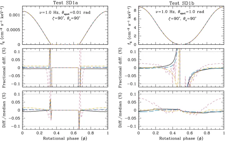
Figures 5–7 show the results of TestsSD1a-f. In all instances, the IM code was used as a reference against which the other codes were compared. It is apparent that all codes perform extremely well in these tests—for most phases, the flux discrepancies are well within the 0.1% requirement (indicated by the pair of horizontal dotted lines). The most pronounced differences (reaching up to ∼1%) occur near the flux minimum around the ingress and egress as the hot spot is eclipsed by the NS. However, in these cases thefluxes are more than two orders of magnitude smaller than theflux around the pulse maximum. These discrepancies are therefore unimportant
Figure 5.Comparisons of the synthetic pulse waveforms from TestsSD1a and SD1b, the slowly spinning (1 Hz) variations of the SD1 tests (see Table1for the assumed parameters). The point-like (qspot= 0.01rad) and large spot (θspot= 1 rad) are shown on the left and right, respectively. The top panel shows the pulse
waveforms. The middle panel shows the fractional difference between the CU (black), GSFC-M (orange), GSFC-S (blue), and Alberta (purple) photon fluxes compared to the IMflux at each phase bin, expressed as a percentage. In the bottom panel, the IM flux is subtracted from the other fluxes and the result is divided by the median IMflux over all phases. The two horizontal dotted lines mark the target ±0.1% measurement precision. Except near the spot eclipse ingress and egress, where theflux is two orders of magnitude smaller than it is at the peak, the agreement between the codes is significantly better than the target precision.
Table 1
Parameter Values for Waveform Test SD1
Quantity Test SD1a Test SD1b Test SD1c Test SD1d Test SD1e Test SD1f
Number of hot spots 1 1 1 1 1 1
Colatitude of spot center(°) 90 90 90 90 60 20
Angular radius of hot spot(rad) 0.01 1.0 0.01 1.0 1.0 1.0
Colatitude of observer(°) 90 90 90 90 30 80
NS mass(Me) 1.4 1.4 1.4 1.4 1.4 1.4
NS radius(km) 12 12 12 12 12 12
ν at infinity (Hz) 1 1 200 200 400 400
Spectrum of emission Planck Planck Planck Planck Planck Planck
Beaming of emission iso iso iso iso iso iso
Figure 6.Same as Figure5except for tests SD1c and SD1d, which consider more rapid rotation(ν = 200 Hz).
Figure 7.Same as Figure5but for comparisons of the synthetic pulse waveforms from TestsSD1e and SD1f, which consider a rapidly spinning (400 Hz) neutron star and more general combinations of colatitude and viewing angle.
for practical purposes. Overall, the tested waveforms agree with each other, and with analytical results where appropriate, to significantly better than the 0.1% target precision.
4.3. Waveform TestSD2: Rotating NSs with Isotropic Narrow Line Emission
For our second set of comparisons we computed phase-energy waveforms assuming that the emission spectrum is confined to narrow lines. This enables tests of the following aspects of the codes.
1. Gravitational and special relativistic redshifts. Because the photon energy at emission is known precisely, it is possible to compute analytically the received energy as a function of the phase of emission and the rotational frequency of the star.
2. Light deflection and time delays. Using a sharp line, especially from a small spot, it is possible to compute from tables the observed phases spanned by the eclipse. This provides an additional test of the computation of light bending and time delays.
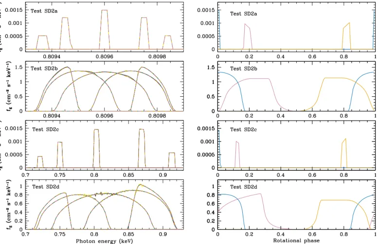
Figure 8.Left: results of the emission line tests SD2a–SD2d (from top to bottom, respectively) for five representative spin phases (f = 0.25, 0.125, 0, 0.75, and 0.875, in order of increasing photon energy of the observed line) for the CU (black), IM (yellow), GSFC-M (orange), GSFC-S (blue), and AB (purple) codes. The spikiness evident in the spectra at some phases for the CU and IM codes is produced due to inexact interpolation of the line profiles. This interpolation problem is not an issue for realistic smooth spectra. Right: for test SD2a and SD2b the monochromatic pulse profiles at energies 0.8094 keV (produced by the AB code and shown in purple at f ≈ 0.2), 0.8096 keV (produced by the GSFC-S and shown in blue at f ≈ 0), and 0.8098 keV (produced by the GSFC-M and shown in orange at f ≈ 0.8) are shown. For tests SD2c and SD2d, the monochromatic profiles at energies 0.75 keV (AB, purple), 0.8 keV (GSFC-S, blue), and 0.9 keV (GSFC-M, orange) are shown. Due to the narrow band nature of the emission lines, at a given photon energy in the observer rest frame the spot emission is only observed at some rotational phases.
Table 2
Parameters of Waveform Test SD2
Quantity Test SD2a Test SD2b Test SD2c Test SD2d
Number of hot spots 1 1 1 1
Colatitude of spot center(°) 90 90 90 90
Angular radius of hot spot(rad) 0.01 1.0 0.01 1.0
Colatitude of observer(°) 90 90 90 90
NS mass(Me) 1.4 1.4 1.4 1.4
NS radius(km) 12 12 12 12
ν at infinity (Hz) 1 1 400 400
Spectrum of emission line Planck line Planck line Planck line Planck
Temperature of emission(keV) 0.35 0.35 0.35 0.35
3. Gravitational lensing. The intensity observed at a given phase also depends on the lensing factor d cosα/d cos ψ. This can be compared with the computed intensity. 4. The capacity of the codes to deal with lines with sharp
energy profiles. No surface atomic lines have yet been confirmed from any NS, but if one were seen then it would provide valuable information. Real line profiles will not be sharp, but tests involving sharp lines stress the codes as much as possible.
We tabulate the model parameters in Table2.
We assume that the emission line has the specific intensity of a Planck spectrum with kTeff=0.35 keV (as measured in the surface comoving frame) within a very narrow energy band, and zeroflux outside of that band. For the 1 Hz tests the energy band was 0.99998–1.00002 keV as measured in the surface comoving frame, the model output was for 200 photon energies, as seen by a distant observer, uniformly spaced in the range 0.809–0.81099keV, and the pulse waveforms were split in 128 equally spaced phase segments. For the 400 Hz tests the energy band was 0.995–1.005keV as measured in the surface comoving frame and the simulations were performed for 200 photon energies, as seen by a distant observer, that were uniformly spaced in the range 0.7–1.0keV. In all cases comparisons were performed between the calculated photon fluxes, which were reported in units of photonscm−2s−1keV−1.
Figure8shows a comparison of the emission line outputs as a function of energy forfive representative spin phases: f=0, 0.125, 0.25, 0.75, and 0.875. It is apparent that the codes are in good agreement, meaning that the emission lines are correctly translated to the observer’s frame. For Tests SD2a and SD2c, the agreement between the linefluxes are exceptional, typically
well within∼0.1% aside from a small number of outliers (∼10 out of 25,600 and 38,400 values for SD2a and SD2c, respectively) for the CU and IM codes.
5. OS Code Verification Tests
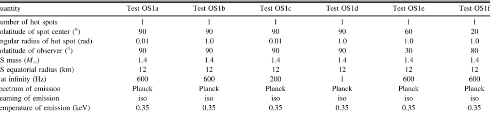
Following the same strategy as in the S+D case, we have devised a series of comparison exercises to test different aspects of modeling hot spot emission in the OS approx-imation. These include consideration of both point-like(0.01 rad) and extended (1 rad) hot spots. In addition, for a subset of tests, we introduce non-isotropic surface emission using simple cos2σ and sin2σ beaming patterns. As in the S+D tests, we assume the same NS with M=1.4 Me at a distance of D=200 pc, with a kT=0.35 keV Planck spectrum hot spot. Because the star is now oblate, the value for the NS radius that we quote is the circumferential equatorial radius Req. We again consider monochromatic pulse profiles at 1 keV in units of photons cm−2s−1keV−1. We note that for a subset of tests, we consider spin frequencies of 600 Hz, which as pointed out in Section 3.3 falls in a regime where the OS approximation introduces errors at the level of a few percent. Nevertheless, for the purposes of the code verification comparisons, considering such rapid spin provides enhanced sensitivity to any dis-crepancies in the implementation of the stellar oblateness and special relativistic effects, because they are much more pronounced for faster spins.
The setup of the series of tests is summarized in Tables3and 4, while the results of the OS code comparisons are illustrated in Figures 9–14. The IM code was again used as a reference against which the other codes were compared. In these OS tests, results from the AMS codes (see Appendix B) are also
Table 3
Parameter Values for Waveform Test OS1 a-f
Quantity Test OS1a Test OS1b Test OS1c Test OS1d Test OS1e Test OS1f
Number of hot spots 1 1 1 1 1 1
Colatitude of spot center(°) 90 90 90 90 60 20
Angular radius of hot spot(rad) 0.01 1.0 0.01 1.0 1.0 1.0
Colatitude of observer(°) 90 90 90 90 30 80
NS mass(Me) 1.4 1.4 1.4 1.4 1.4 1.4
NS equatorial radius(km) 12 12 12 12 12 12
ν at infinity (Hz) 600 600 200 1 600 600
Spectrum of emission Planck Planck Planck Planck Planck Planck
Beaming of emission iso iso iso iso iso iso
Temperature of emission(keV) 0.35 0.35 0.35 0.35 0.35 0.35
Table 4
Parameter Values for Waveform Test OS1 g-l
Quantity Test OS1g Test OS1h Test OS1i Test OS1j Test OS1k Test OS1l
Number of hot spots 1 1 1 1 1 1
Colatitude of spot center(°) 60 60 20 20 90 90
Angular radius of hot spot(rad) 1.0 1.0 1.0 1.0 1.0 0.01
Colatitude of observer(°) 30 30 80 80 90 90
NS mass(Me) 1.4 1.4 1.4 1.4 1.4 1.4
NS equatorial radius(km) 12 12 12 12 12 12
ν at infinity (Hz) 600 600 600 600 600 600
Spectrum of emission Planck Planck Planck Planck line Planck line Planck
Beaming of emission cos2σ sin2σ cos2σ sin2σ iso iso
included; in addition to the “star-to-observer” ray-tracing technique described here, the AMS codes can also employ “observer-to-star” (i.e., image plane) ray tracing based on the prescription from Psaltis & Özel (2014). For the intended purposes the two approaches to ray tracing produce results that are virtually indistinguishable. As with the S+D tests, for most rotational phases, the deviations in computed photon flux are comfortably below the 0.1% requirement. The exceptions are phase bins around the ingress and egress as the hot spot is occulted by the NS. However, in these cases the photonfluxes are minuscule, being more than two orders of magnitude smaller than theflux around the pulse maximum. Based on this, we deem these discrepancies to be unimportant for practical purposes. Specifically, in actual observational data, the measured flux at pulse minimum will typically be dominated by other source emission components or non-source back-ground. Even in the event of negligible background, the measurement uncertainty of the low count rate at the spot ingress/egress would dominate over a ∼0.1% numerical imprecision. Finally, the likelihood functions used for para-meter estimation based on the pulse profile modeling technique are generally insensitive to error at phases in the vicinity of ingress/egress.
6. Conclusions
We have described the model of hot spot emission from a rapidly rotating neutron star that we intend to apply to NICER X-ray data of MSPs. We have presented the results of thefirst
direct comparison between independently developed codes to allow a crucial consistency check of the calculations that go into a model of emission from a rapidly rotating NS in both the S+D and OS approximations. We find that the outputs of the codes are in excellent agreement with one another and with several analytical and semi-analytical results, with fractional differences of0.1%. In addition, we obtain consistent results with the“star-to-observer” and “observer-to-star” (i.e., image-plane) ray-tracing techniques (see Appendix B). The set of verified, high-precision reference synthetic pulse profiles for both the S+D and OS comparisons is provided to the community as supplementary material to this article to facilitate testing of other independently developed codes.
A crucial aspect of the comparisons presented in this work is that the synthetic pulse profiles were generated with what we call“practical” versions of the codes, meaning that they strike an optimal balance between providing accuracy at a level better than 0.1% and having short execution times. While, in principle, we could obtain substantially better agreement by increasing the number of resolution elements in the codes, this would come at the expense of extra computational time. For the practical applications of these codes in parameter estimation analyses, for each sampled combination of parameters it is necessary to generate a synthetic pulse profile for hundreds of detector energy channels. With this in mind, the numerical performance of the codes described here has been optimized so that the computation of a synthetic pulse profile at a given energy is executed in much less than 1 s on a single processor
Figure 9.Comparisons of the synthetic pulse waveforms from TestsOS1a and OS1b. The point-like (θspot= 0.01 rad) and large spot (θspot= 1 rad) are shown on the
left and right, respectively. The top panel shows the pulse waveforms. The middle panel shows the fractional difference between the CU(black), GSFC-M (orange), GSFC-S(blue), Alberta (purple), and Amsterdam (green) fluxes and the IM flux at each phase bin, expressed as a percentage. In the bottom panel, the IM flux is subtracted from the otherfluxes and the result is divided by the median IM flux over all phases. The pair of dotted lines show the target ±0.1% measurement precision. Except near eclipses, where theflux is two orders of magnitude smaller than it is at the peak, the agreement between the codes is significantly better than the target precision.
core (see Appendix Bfor details). As demonstrated in Miller et al. (2019) and Riley et al. (2019), the consistency between the codes and their computational efficacy makes them well suited for use in the large-scale statistical sampling runs required to obtain estimates on the M–R relation and the dense matter EoS.
We thank J.Nättilä, F.Özel, D.Psaltis, and J.Poutanen for insightful discussions and code comparisons. This work was supported in part by NASA through the NICER mission and the Astrophysics Explorers Program. M.C.M. is grateful for the hospitality of the Kavli Institute for Theoretical Physics at the University of California, Santa Barbara, during part of the writing of this Letter, and was therefore supported in part by the National Science Foundation under grant No. NSF PHY-1748958. M.C.M. is also grateful for the hospitality of the Perimeter Institute where part of this work was carried out. Research at Perimeter Institute is supported in part by the Government of Canada through the Department of Innovation, Science and Economic Development Canada and by the
Province of Ontario through the Ministry of Economic Development, Job Creation and Trade. A.L.W. and T.E.R. acknowledge support from ERC Starting grant No.639217 CSINEUTRONSTAR (PI Watts). S.M.M. thanks NSERC for research funding. This research has made extensive use of NASA’s Astrophysics Data System Bibliographic Services (ADS) and the arXiv.
Software: MATPACK(http://www.matpack.de), Python/ Clanguage(Oliphant 2007), GNUScientificLibrary(GSL; Gough 2009), NumPy(van der Walt et al. 2011), Cython (Behnel et al.2011).
Appendix A Parameter Notation
Here we provide a summary table that defines the notation for the numerous symbols used throughout this Letter, which for many parameters differs from previous publications. For convenience, Table5 lists each symbol and a brief definition.
Figure 11.Same as Figure9but for tests OS1e and OS1f.
Figure 13.Same as Figure9but for tests OS1i and OS1j.
Figure 14.Left: results of the emission line tests OS1k and OS1l(from top to bottom, respectively) for five representative spin phases (f = 0.25, 0.125, 0, 0.75, and 0.875, in order of increasing photon energy of the observed line) for the CU (black), IM (yellow), GSFC-M (orange), GSFC-S (blue), and AB (purple) codes. The spikiness evident in the spectra at some phases for the CU and IM codes is produced due to inexact interpolation of the line profiles. Right: monochromatic pulse profiles for the OS1k and OS1l tests at energies 0.75 keV at f≈0.125 (from IM code, marked in yellow), 0.8 keV at f≈0.0 (from GSFC-S code, marked in blue), and 0.9 keV atf≈0.8 (from AB code, marked in purple). Due to the narrow band nature of the emission lines, at a given photon energy in the observer rest frame the spot emission is only observed at some rotational phases.