Performance simulation of a hybrid geothermal rain water tank coupled to a building mechanical ventilation system

HAL Id: hal-03247213

https://hal.archives-ouvertes.fr/hal-03247213

Submitted on 2 Jun 2021

HAL is a multi-disciplinary open access

archive for the deposit and dissemination of

sci-entific research documents, whether they are

pub-lished or not. The documents may come from

teaching and research institutions in France or

abroad, or from public or private research centers.

L’archive ouverte pluridisciplinaire HAL, est

destinée au dépôt et à la diffusion de documents

scientifiques de niveau recherche, publiés ou non,

émanant des établissements d’enseignement et de

recherche français ou étrangers, des laboratoires

publics ou privés.

Performance simulation of a hybrid geothermal rain

water tank coupled to a building mechanical ventilation

system

Jean-Baptiste Bouvenot

To cite this version:

Jean-Baptiste Bouvenot. Performance simulation of a hybrid geothermal rain water tank coupled

to a building mechanical ventilation system. Building Simulation 2021, Sep 2021, Bruges, Belgium.

�hal-03247213�

Performance simulation of a hybrid geothermal rain water tank coupled to a building

mechanical ventilation system

Jean-Baptiste Bouvenot

1

National Institute of Applied Sciences of Strasbourg, HVAC department, Strasbourg, France

2

The Engineering science, computer science and imaging laboratory (ICube lab), Illkirch, France

Abstract

Large buried rain water recovery tanks are similar to single but large superficial geothermal probes that can be “thermally activated” by immersion of a heat exchanger. This hybrid concept is poorly studied in the literature. This publication presents the heat exchanger sizing and the energy relevance of a rainwater tank used as water supplier and as geothermal probe in a heat recovery double-flow mechanical ventilation unit to cool down fresh air in summer and to preheat cold air in winter. The system has been stressed in actual and future climates (Strasbourg climate, France) by testing different control strategies. This study shows the good performance of this passive and low tech system to provide sufficient passive cooling in summer peak days (>1000 W for 8 m3 buried tank) while relieving the sewage and water supply network. This study proves it’s a promising hybrid concept which can be spread in different areas (urban or rural) in a climate change and natural resources depletion context.

Key Innovations

• a new low tech and passive concept of hybrid geothermal rain water tank is modelled.

• a geothermal rain water tank can supply significant cooling power during heat waves (>1 kW)

• the concept has been stressed in future climates (2100) and still present good performances.

Practical implications

This kind of model requires at least 5 years of time simulation and requires to be stressed in future climate because of their long lifetime.

Introduction

In the current context, due to climate change (frequent and intense heat waves) (IPCC, 2020) coupled with new and drastic thermal regulations, summer comfort in buildings with a low environmental impact becomes an essential problem. In this context, active air conditioning systems should be avoided as far as possible in order to:

• avoid significant GHG emissions (refrigerants, electrical consumption, etc.),

• limit the building’s energy needs,

• avoid amplifying the urban heat island effect. In addition, the climate tends towards a decrease in rainfall in a major part of the world (including France) and an increase in temperatures, mainly in summer

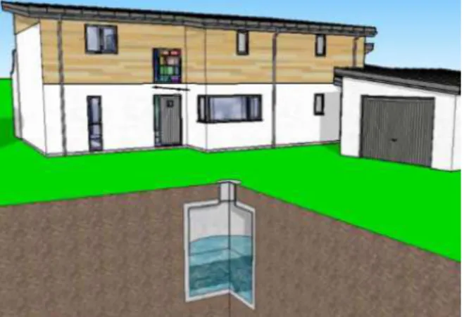
(Meteo France, 2020). The idea here is to be part of an energy efficiency strategy based mainly on passive low-tech systems. Passive and low-low-tech solutions are then found to be relevant in urban environments to both limit the heat island effect and maintain thermal comfort in buildings during intense heat waves without amplifying it. In addition, the French agency for ecological transition states that very low temperature geothermal renewable energy is an underdeveloped area and thus wishes to promote it (Cardona-Maestro, 2016). Thus, we will focus here on rainwater tanks (RWT) from a roof or drainage system with multiple interests (see Figure 1). Indeed, they allow a certain autonomy regarding the water needs and relieve the sewage networks in case of rainy episodes as well as the public drinking water resource in a context of more frequent summer droughts. These tanks can be above-grounded or buried. Large underground tanks (several m3) can then be assimilated to unique but large exchange area geothermal probes that can be thermally activated by the immersion of a heat exchanger (HX). This is a semi-passive, low-tech geocooling solution that limits the use of active air conditioning systems. In addition, a preheating of the new air can also be done in winter to avoid the frost of the double flow HX and to store cold thermal energy for a summer use. Thus, an immersed HX in the tank and connected to an HX sheathed in a double flow air network would make it possible to pre cool fresh air.

It appears these systems have been poorly studied in the literature; the only devices studied experimentally incorporate directly ventilation pipes immersed in tanks (Choorapulakkal, 2013); were connected to hydraulic floor (Kalz, 2010) (no modelling); were connected to a

heat pump with a tank fitted by metallic fins (Gan, 2007) or used a drainage zone to exploit rainfalls (Gao, 2016). Other authors study numerically basic concepts of geothermal lakes (Yumrutas, 2000 and 2005) or only propose concepts without proving their performance (patents) (Irei, 2001; Bagot, 2009).

Method

The aim is to develop a model to prove the performance of these systems before being validated with in situ tests on prototypes. The particularity here is that the water level is variable according to the water withdrawals of inhabitants and rainfalls fillings even if there is a minimum water level to maintain the pump immersed. This minimum volume can be also considered as an energy guard volume. In order to model the geothermal hybrid system (buried tank coupled to a HX), a numerical model of this system in a study case using a simplified 2D model in axisymmetric cylindrical coordinates was developed. The model is split as follows:

• the tank: represented by a double zonal model on the water volume and on the air volume (see Figure 2); • the soil: represented by a model discretised by the finite volume method (see Figure 4);

• RWT water/water HX: represented by an analytical model (see Figure 2).

Finally, the coupling of the 3 parts with a double flow mechanical ventilation system (DFMVS) will be carried out. The performances of the system will be assessed in winter and mainly in summer to compute cooling capacities during hot periods. The simulation will be run over 5 years to reach the stabilization on model outputs. Coil heat exchanger in the tank

At first, we assessed the minimum length of the coil HX in order to reach a thermal efficiency Eww of 0,8. We

began by assessing the forced internal convection coefficient in the coil. The critical Reynolds number

Recrit (Incropera, 2011) gives the limit between the

turbulent and the laminar regime for this coil HX:

= 2300 1 + 12 , (1)

For the laminar flow regime in a coiled HX (constant heat flux density boundary condition), the most reliable correlation to compute Nusselt number Nu is supplied by Manlapaz et al. (1980) which involves the Dean number

De and the helical number He:

= , and = 1 + _" ℎ_,#$ (2) %& , = ⎣ ⎢ ⎢ ⎢ ⎢ ⎢ ⎢ ⎡ ⎝ ⎜ ⎜ ⎜ ⎜ ⎛ 48 11 + 51 11 1 + 0 1342 12 , $3 $ ⎠ ⎟ ⎟ ⎟ ⎟ ⎞ 7 + 1,816 9 1 + 1,15₁₂ , : ;.= ⎦ ⎥ ⎥ ⎥ ⎥ ⎥ ⎥ ⎤ ; 7 (3)

For the turbulent regime, a reliable Nusselt number correlation for coiled HX is given by Rogers (1964):

%& , = 0,023 C,D=12C,E, ,# C,;

(4) All the thermal properties are computed by considering glycol water with a glycol rate of 30 % and a mean glycol water temperature

F

correlation of Xin (1996) who proposes a correlation taking into account the orientation of the coil axis:

I < 10=_{: L}vertical coil ∶ %& , = 0,290 IC,$W7 horizontal coil: %& , = 0,318 IC,$W7 (5)

The outer surface temperature is computed by Eq. 6:

F , ≈ ℎ , , , FH+ FH+ FGH, − FGH, ln _FF_GH,GH, − F_{− F}H_H# 1 ℎ , , , + ln , , # 2\ ]]^ ℎ , , , + 1 1 ℎ , , , + ln ,_,# 2\ ]]^ (6)

Finally, we compute the efficiency of the coil HX Eww

thanks to the coil length which is chosen to reach at least 0,8 on average (we found a copper pipe length

_ required of 75 m): `a = "_ 1 ℎ , , , + ln ,_, # 2\ ]]^ + 1 ℎ, , , (7) bHH= 1 − c defg hijklm_{no with q} rGH= 12 l. minc; (8) Water loop

The coil HX inlet and outlet temperatures (see Figure 2) is computed by assuming the quasi static state:

FGH, =FGH,_{1 − b}− bHHFH HH (9) FGH, = ht ]qrm _ubvHFu + ht ]qrm_GHbHHFH 1 − bHH ht ]qrm_u bvH+ ht ]qrm_GHbHH 1 − bHH with bvH= 0,8 (10)

The coil HX efficiency is updated at each time step according to temperature fields of the systems. We assumed the ducted glycol water to air HX (before the double flow HX mechanical ventilation system) has a constant efficiency b_vH because of forced convection on both sides and because we use a commercial system which provides information for nominal conditions. Thermal balance on the water volume

We assume the water zone is isothermal but get a variable water volume (Vw) and we do a thermal balance

(see Fig.2 and Eq. 11) to get dynamically its temperature

tH ]H wHFH= xyv z

+ xy{ H−xy^rv] −xy|] z}−xy −xy ||,H,r− xy ||,H, −xyr−xyv{−xy −xy~

(11)

We solve this equation by using an exlicit schema. The heat flux extracted from the water volume to the glycol water loop is computed by equation 12:

xy = •tGH ]GHqrGHhF , cF ,m with qrGH= 2. 10cE m7. sc;

(12)

The control strategy is based on a ON/OFF controller with two seasonal limitations (winter and summer):

•• = 0 if Fƒ ze„ < Fu < Fƒve„

• = 1 if not (13)

The radiative flux is computed by using the Stefan-Boltzmann law and a surface weighted mean reference temperature of walls that see the water surface:

xyv{= …H†aH hFHE− FE^~,Hm (F in ‡) with: F^~,H=av F_av + avrFvr

v + avr

(14)

The convection flux is computed by using a simplified correlation depending on the mean air speed of the air cavity which is considered as sheltered (Auer, 1996):

xyr= ℎvHaH (FH− Fv) with: ℎ vH= 3,1 + 4,1&vC,= and &v= 0,5 m. sc;

(15)

Each thermal flux linked to the water –drawing or water-harvesting will be computed as an advection flux:

xyv z= ˆy v z ]HFv z with Fv z= Fu ˆy v z= tH. 2I ‰. a ~. Š ~

with Š ~= 0,9 and a ~= 100 m² here

(16)

The outdoor air temperature Tout is cooled down during

rainfalls because of evaporative cooling effect. The meteorological files (measured or modelled in MeteoNorm software) naturally take into account this effect. The heat flux linked to the tank filling when the water level is too low is computed with a district cold

water (DCW) temperature model coming from in situ measurements (ADEME, 2016). The aim is to keep an energy guarded water volume and to maintain the pump drought (5 m3 here for a total volume of 8 m3):

xy{ H= ˆy{ H ]HF{ H with ∶ F{ H= 17 + 3• ‰ Ž2"( /3600 − 730)₈₇₆₀ • and ‘ˆy{ H= tHwƒ z_’− wH if wH< wƒ z

ˆy{ H= 0 if not

(17)

The sprinkling heat loss linked to gardening or car washing is computed only in the hot period:

xy|] z}= ˆy|] z} ]HFH with:

“ˆy|] z}=0,1 _{60 kg. s}c; if 5.3600.30.24 < < 8.3600.30.24

ˆy|] z}= 0 if not

(18)

The mass flow has been computed according to national statistics (6% of the water consumptions) and is assumed to be continue over 3 months that explains the relatively low value. This flow-rate is equivalent to a value of 1 m3.week-1. We apply the same strategy for the heat flux linked to sanitary water needs by considering a constant extraction over the whole year with a volume-flow rate representing 20 % of the global water consumption.

xy = ˆy ]HFH with: ˆy = 0,02 kg. minc;_{. pers}c;_{(≈30 l.day}-1

.pers-1) (19)

If the rain water volume reaches the highest level in the tank, an overflow (of) will be rejected by a specific network that will induces a heat flux:

xy ~= ˆy ~ ]HFH with: “ˆy ~= tHwH− w_’ ƒv if wH> wƒv

ˆy ~= 0 if not

(20)

Then, the evaporation heat losses are computed thanks to vapour pressure difference between a saturated air at water temperature at the air/water interface and the vapour pressure of the air far from the surface. Shah (2014) established an exhausted review on evaporation heat and mass losses correlations and give preconisation for closed vessels (correlation of Hens (2009)):

xy^rv]= ˆy^rv]_r with:

ˆy^rv]= 4,09bcC=aH ˜ |v(FH) − rv](Fv)™ With: _rv](F_v) = 2ℎ_{v |v}(F_v)

(21)

The conduction losses through all the vertical and horizontal walls are computed thanks to the finite volumes method which supplies the weighted mean wall temperature Fš_Hr:

xy ||,H,r= ℎ ,HraHr(FH− FšHr) (22)

The inside vertical natural convection coefficient on wet walls is updated at each iteration by using the following formula from Incropera (2011):

› %&Hr= 0,115 IrC,77 if IHr> 10W %&Hr= œ 212Hr 5h1 + 2•12Hr+ 212mž C,$= IHrC,$= if IHr≤ 10W (23)

We compute with a similar approach horizontal heat losses through wet walls:

xy ||,H, = ℎ ,H aH (FH− FšH ) with: (24) Figure 2: System description and thermal balance.

For the convection exchange coefficient ℎ _,H , we use the following formula from Incropera (2011):

›if FH< FšH : L%&H = 0,54 IH C,$= _{if I} H < 10 %&H = 0,15 IHC,77 if IH > 10 if not ∶ 0,27 IHC,$= (25)

All the convection exchange coefficients are updated at each time step to take into account the water level variation and the thermal properties are computed at the film temperature.

Thermal balance on the air volume

Eq. (26) gives the thermal balance of tha air zone in unsteady state. It is to note the evaporation heat flux which is extracted from water is not given to the air because this flux is turned into steam. This steam will be taken into account in the mass balance of the air zone. We only consider the sensible part of this heat flux

xy|^z|,^rv]which is insignificant here.

tv ]v{¡_{¢£¢= xy|^z|,^rv]+ xyr+ xyv{+xy u − xyv− xy ||,v,r−xy ||,v, = ˆy^rv] ]rFH+ ℎ vHaH (FH− Fv) + …H†aH hFHE− FE^~,Hm+(ˆyu + ˆyv ) ]vFu − (ˆyv+ ˆyv ) ]vFv− xy ||,v,r−xy ||,v,

(26)

The variable air volume Va will be computed thanks to

the mass balance (see Figure 3). Then, the convection and radiations fluxes coming from the water zone become incoming fluxes here. There are 2 advection heat fluxes linked to the filling and emptying of the RWT. The air volumes empties when the water level increases which will drive the air away as a piston and at the contrary will admit outside air when the water level will decrease. In addition, an air change rate τ is assumed linked to the air leakages.

xyu = (ˆy u + ˆyv ) ]vFu with ∶ ˆy u = › ˆy u = tvwH c_{− w} H ’ = tvwv− wv c ’ # if wHc− wH> 0 ˆy u = 0 if not and ˆyv = ¤wv (27)

When the RWT tank fills, it expels the air assumed incompressible. In addition, an air change rate τ is assumed linked to the air leakages.

xyv= (ˆyv+ ˆyv ) ]vFv with: ˆyv= › ˆyv= tvwH− wH c ’ = tvwv c_{− wv} ’ # if wH− wHc> 0 ˆyv= 0 if not and ˆyv = ¤wv (28)

The heat losses between the air zone and the soil are computed with the same approach and the same formula than for the water zone, the difference being that the characteristic length for the vertical convection coefficient will be zgr-zw (see Figure 2) and that the

thermal properties will be the air properties. Mass balances

The mass balance is applied to the air zone and the water zone in order to know the water level zw and to know

dynamically the air and the water volumes Va and Vw at

each time step. The water is assumed incompressible and we consider different mass flows linked to: evaporation to the air zone, withdrawals to building, rain harvesting flow and DCW supply for maintaining the water level to a minimum value:

ˆyH= tHwyH= ˆyv z+ ˆy{ H−ˆy^rv]−ˆy|] z}−ˆy −ˆy~ (29)

wH= w¥c−_i¦_ohˆyv z+ ˆy{ H−ˆy^rv]−ˆy|] z}−ˆy −ˆy ~m (30)

All the mass-flow rates have been computed from Eq. (16) to (21) and from Eq. (27) and (28). Then, we get the water level:

§H=_awH

H (31)

The air volume is complementary with the water volume (the RWT volume being constant), that leads to:

wv= aH (§ƒv − §H) +" H , $

4 h§G − §ƒv m (32)

Moisture balance

The evaporation heat losses term requires to know the vapour pressure of the air in the RWT. We do the moisture balance on the air zone by considering humidity incoming flows from outside, outcoming flows and water evaporation flow:

ˆrv]₌ w¨vvIℎv_{= ˆy}

^rv]+ (ˆy u + ˆyv )Iℎ u − (ˆyv+ ˆyv )Iℎv

Iℎ u = 0,622 rv](Fu)

v ƒ− rv](Fu) with: v ƒ= 101300 Pa

And: _rv](F_u) = 2ℎ _{u |v} (F_u )

(33)

2ℎ u is the relative humidity of outside air given directly by meteorological files. We compute also the relative humidity of the air in the RWT to see the saturated state over the year:

2ℎv=_(C,¬$$-vv ¢]¢ª«_¢) c $7,7$¬=c ®¯°±,² ³¢ c˜´²±,µ¯³¢ ™ ± # (Fv in K) (34)

With, in steady state:

Iℎv=ˆy^rv]+ (ˆy_ˆy u + ˆyv)Iℎ u v+ ˆyv

(35) Figure 3: Mass balances on the 2 fluid zones.

We will assume a quasi-static state in the calculations to get the absolute humidity of the air zone to avoid divergence problem with the explicit scheme and because the time constant is tiny in comparison with global dynamic of the system. No moisture transfers are taken into account with concrete walls.

Soil

We assume a homogenous material for each material (concrete for the tank and ground with

\G = 1,5 W. mc;. Kc; ) and there are no active water flow

underground. The thermal transfers in the soil obey to the heat equation in cylindrical coordinates:

t ]¸F_{¸ = \ Ž}¸²F_{¸§² +}¸²F_{¸2² +}1₂¸F_¸2• (36)

We use the finite volumes method using the unique following equation valid for each node by adapting the spatial steps and the thermal properties according to the location of the node (we used the cardinal points notation to identify the cells relative position (N, S, E and W for North, South, East and West):

F = Fc_{+ ¹º(F} ºc− Fc) + ¹¥(F¥c− Fc) + ¹»(F»c− Fc) + ¹e(Fec− Fc) + a With: ⎩ ⎪ ⎪ ⎨ ⎪ ⎪ ⎧ ¹º= 9 1 + ∆2₂₂ ’2º 2\º+ ’22\ :_{t ’2}’ ¹¥= 9 1 − ∆2₂₂ ’2¥ 2\¥+ ’22\ :_{t ’2}’ ⎩ ⎪ ⎪ ⎨ ⎪ ⎪ ⎧ ¹»= 9_’§ 1 » 2\»+ ’§2\ :_{t ’§}’ ¹e= 9_’§ 1 e 2\e+ ’§2\ :_{t ’§}’ a =_{t ’§}Á’ (37)

The source term S is only applied on the superficial nodes in contact with outside air to take into account the solar radiation Á in W.m-2

.

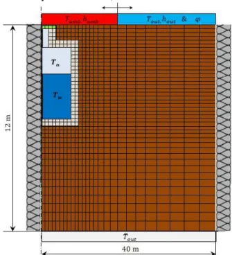
Boundary conditions

As it’s shown on figure 4, we consider adiabatic boundary conditions on the vertical boundaries, an imposed temperature (the annual mean temperature Fšext

computed according to the chosen meteorological file) at the bottom at 12 m of depth and superficial exchange at the top. At the top, there are 3 boundary conditions. If a building is built above the RWT, we assume a superficial exchange with an ambient temperature Tamb

of 20 °C in winter and of 28 °C in summer (june, july and august) with a linear variation between the transition months in spring and in autumn. The superficial exchange coefficients hamb and hout are assumed constant

at 7 W.m-2.K-1 indoor and at 25 W.m-2.K-1 outdoor. Mesh

The mesh is regular with a constant step of 5 cm in the RWT zone with a geometrical progression in radial and vertical directions with a ratio of 1,1 that limits the mesh size that is important to threshold the simulation time which is made over 5 years with a hourly time step. The meshed zone is 12 m deep and 80 m large with a radius of 40 m (see Figure 4). The model is made to be easily adapted to take in consideration insulation layer for

example or variable thermal properties like thermal conductivity to take into account their variation along the season (for example the ground thermal conductivity can vary significantly with the moisture content which can be very low in summer).

Control strategy

The control strategy is simply carried by using ON/OFF controller which triggers on the glycol water loop when the outside air is lower (in winter) or higher (in summer) than set points (SP). Several set points will be tested:

• operation in summer only when Text > Fƒve„ ;

• operation in summer (Text > Fƒve„ ) and in winter (Text

< F_{ƒ z}e„);

The main monitored output will be the water temperature Tw we want to threshold below 20°C to

ensure a sufficient cooling capacity during summer temperature peaks. With an intermediate glycol water loop, there are 2 temperature pinches to fight that requires maintaining a sufficient low temperature in the tank to cool down significantly the fresh air.

Simulation hypothesis

We built a complete model but we propose here to firstly prove the performance of the system in unfavourable conditions. We decided to maintain the water level at the minimum level in order to maintain a level sufficient to keep the pump submerged. The studied tank presents a total volume of 8 m3 that is suitable for residential buildings applications but we considered only 5 m3 of water inside. Besides, we assume constant thermal properties over the year for materials and we consider no house above the RWT. Finally, we used Meteonorm software meteo data files for 2010-20 periods and future climate data by considering the most pessimistic IPCC scenario for 2100 (IPCC; 2020) and we apply the model for the Strasbourg (France) climate (mean temperature of 11 °C and average rainfalls of 700 mm per year (see Figure 7 for the temperature profile).

Results

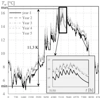
Figure 5 shows the temperature field in the soil at a given time influenced by the RWT. At the initial moment the temperature field being unknown, it has been uniformly set at 9 °C. Figure 6 shows the evolution of water temperature in the RWT over 5 years and shows that it is required to simulate at least during 3 years to reach the stabilization of the temperature field in the soil, with years 3, 4 and 5 being almost stacked. The idea is then to make a simulation of 5 years and keep only the last year to analyse the results. The simulation was done with the Strasbourg weather file generated by the Meteonorm software (in 2010-2020 and in 2100). In the reference case (see Figure 6), we found a reasonable range of 11,3 K over the year, a minimum value of 5,4 °C, which prevents water from freezing even if heat is extracted in the winter, and a maximum value of 16,7 °C, which is tempered despite heat reinjection in the summer. The maximum power obtained in summer is 1083 W (see Table 1).

Figure 5: Temperature fields.

Figure 7 results were obtained for a control strategy that operates the system for Text < 8 °C or Text > 24 °C. It

shows that the system prevents icing and allows to avoid using the anti-frost electric heating resistance of the DFMVS. Table 1 summarizes the results of the parametric study by considering current and future weather and considering different control strategies. For the calculations, we consider a housing of 100 m² on floor and a pump power of 20 Wel based on a calculation of pressure drop on the coil HX and preheating water/air HX manufacturer data. Table 1 shows, respectively, the minimum Tmin and maximum Tmax water temperatures

obtained in the RWT, the maximum heating or cooling powers generated per season Pmax, the amount of

absolute heat Q and specific heat Qspe recovered from the

ground or reinjected into the ground, the operating time of the pumps per season top, the primary energy

consumed by the pumps Epump and the seasonal

coefficient of performance (SCOP) of the system.

Figure 7: Evolution of Tout, Tw and Tbl during the 5th simulation year.

4 6 8 10 12 14 16 0 730 1460 2190 2920 3650 4380 5110 5840 6570 7300 8030 8760 T_w[°C] t [h] year 1 Year 2 Year 3 Year 4 Year 5 11,3 K -8 -4 0 4 8 12 16 20 24 28 32 0 730 1460 2190 2920 3650 4380 5110 5840 6570 7300 8030 8760 T [°C] t [h] Tw Text Tas

T

T

T

Table 1: System performances according different configurations. C li m a te Control strategy (ON if…) Season Tmin [°C] Tmax [°C] Pmax [W] Q [kWh/an] Qspe [kWh/m²/an] top, [h] Epump [kWhPE/an/m²] aÂÃ1 Ž=2,58 b_b |]^ ]uƒ] • [-] S tr as b o u rg 2 0 1 0 -2 0 2 0 Tout>24 and Tout<8°C summer - 16,7 1083 229 2,3 301 0,2 38 winter 5,4 - -681 -715 7,1 2719 1,4 13 Text>24 summer - 17,0 1044 222 2,2 301 0,2 37 winter 9,9 - - - - S tr as b o u rg 2 1 0 0 Text>24 and Text<8°C summer - 20,7 1051 442 4,4 732 0,4 30 winter 5,9 - -772 -742 7,4 2421 1,2 15 Text>24 summer - 20,8 1039 430 4,3 732 0,4 29 winter 10,8 - - - - - - -

Discussion

It can be seen that the water in the RWT never freezes and that the heat regeneration of the soil in winter has a very small impact on the peak temperature of the water in summer (in the range of 0,1 K). Winter operation, despite the energy consumption of the pump, is nevertheless relevant to avoid using the anti-frost electrical resistance. The primary energy consumption avoided by the electrical resistance is 71 x 2,58 kWhPE or 1,8 kWhPE/m²/year: value slightly higher than the winter consumption of the pump. Also, for the simulations carried out with a future climate, we see that the cooling powers are slightly lower although the increase of the water temperatures increases significantly by the order of 4 K compared to outside temperatures which increases by an average of 2 K in the 2100 scenario. With higher outdoor temperatures, with equal control strategy, the system is more stressed in terms of operation time, which re-injects more heat into the volume of water. This explains the marked rise in the maximum RWT temperature for the 2100 future climate. Finally, the primary energy consumption of the system in operation in summer is negligible, but in the end the system provides sensitive specific cooling energy of the order of 2 to 3 kWh/m2/year for the current climate and 4 to 6 kWh/m2/year for the future climate.

Conclusion

A new numerical model of a hybrid and innovative geothermal rain water tank was developed to assess its energy relevance when coupled to a double flow mechanical ventilation system. The goal is to avoid using active air conditioning while guaranteeing summer comfort. The simulations have shown that its performance allowed to cool down the outside air during the summer peaks temperature from 5 to 10 K with cooling powers of the order of 1 kW. This order of magnitude is interesting but remains modest in terms of the usual rules of air-conditioning design requiring around 50 W/m². However, this system does not pretend to replace an air conditioning system but allows to make cooling to avoid a possible use of air conditioning. The model also shows good performance considering warmer future climates (2100). It also shows that it is preferable to use the system in winter to avoid using anti frost control systems, but also to reload the ground in cold

thermal energy for the summer season. In current climate, it limits blowing temperature below 26 °C for outside temperatures up to 34 °C. We also size a coil HX suitable to this application (length of at least 75 m of copper pipes for 8 m3 RWT volume). In perspective, it would be interesting to couple this model with a dynamic energy building model to quantify the comfort obtained with this system. In addition, it would be interesting to add a precipitation and withdrawals flow models to assess the impact of filling and emptying water the RWT which should tend to improve the theoretical performance of the system. Finally, further parametric studies are underway to assess the impact of geometry (size, material, depth of burial, thermal insulation of the upper part of the RWT), water level variation, control strategy, and the variation of the physical/thermal properties of the ground. The next step is the validation of this model thanks to a prototype and in situ data.

Acknowledgement

Nomenclature

Lv vaporization latent heat, J.kg-1

ˆy mass-flow rate, kg.s-1

Nu Nusselt

number,-Pitch coil pitch, m

Pr Prandtl number, - p pressure, Pa x heat, J or kWh xy heat flux, W qv volume-flow, m3.h-1 rain rainfalls, m.s-1 Ra Rayleigh number, - rh relative humidity, - S surface, m² Fš mean temperature, °C or K U thermal conductance, W.m-2.K-1 u fluid speed, m.s-1 V volume, m3

Subscripts and exponents

ah horizontal RWT walls in contact with the air

av vertical RWT walls in contact with the air

aw air/water

bl blown air

cv convection

dcw district cold water

evap evaporation

gr ground

gw glycol water

h horizontal

i inner side of the coil HX

LM logarithmic

o outer side of the coil HX

of overflow

out outside

PE primary energy

rad radiation

ref wall reference temperature for radiation

sat saturated vapour

sens sensible

toil toilet

v vertical or vapour

vap vapour

w water (in the tank)

wh referstoRWThorizontalwallsincontactwithwater

wv refersto RWT vertical walls in contact with water

ww water/water heat exchanger Greek symbols ∆ time step, s ∆2 radial step, m ∆§ vertical step, m • controller output (0 or 1),-ε infrared emissivity,- φ solar flux, W.m-2 λ thermal conductivity, W.m-1.K-1 ρ density, kg.m-3 σ Stefan-Boltzmann constant, W.m-2.K-4

τ air change rate, h-1

¨ specific volume, m3.kg-1

References

ADEME, (edited by ADEME) (2016). Vers une meilleure connaissance des besoins en eau chaude sanitaire en tertiaire, Technical guide

Auer, T. (1996). TRNSYS-TYPE 344, Assessment of an indoor or outdoor swimming pool, TRANSSOLAR Energietechnik GmbH.

Bagot J. et al. (2009). Procédé et dispositif de réservoir tampon thermique pour le préchauffage et le rafraîchissement des locaux, European patent

FR2948179A1

Cardona-Maestro, A. (2016). Etude sur la géothermie très basse énergie afin de redynamiser la filière,

Etude ADEME

Choorapulakkal, A. and Nogughi, M. (2013). Performance Analysis Of A Proposed ‘Water Tube Heat Exchanger’ Space Cooling System in Kerala,

PLEA2013 - 29th Conference, Sustainable

Architecture for a Renewable Future, Munich,

Germany 10-12 September 2013

Gan, G. et al. (2007). A novel rainwater–ground source heat pump – Measurement and simulation. Applied

Thermal Engineering 27, 430–441.

Gao, Y. et al. (2016). Thermal performance improvement of a horizontal ground-coupled heat exchanger by rainwater harvest. Energy and

Buildings 110, 302–313.

Hens, H. (2009). Indoor climate and building envelope performance in indoor swimming pools. Energy

efficiency and new approaches, Istanbul Technical

University: 543-52

Incropera, F. P. et al. (edited by John Wiley & Sons. ) (2011). Fundamentals of heat and mass transfer. (USA)

IPCC, IPCC reports, https://www.ipcc.ch/srccl/ (accessed the 27/05/2020).

Irei, S. et al. (2001). Air conditioning system for refreshment utilizing rainwater. US patent,

US6227000B1.

Kalz, D.E. et al. (2010), Novel heating and cooling concept employing rainwater cisterns and thermo-active building systems for a residential building.

Applied Energy 87, 650–660.

Manlapaz, R. L., & Churchill, S. W. (1980). Fully developed laminar flow in a helically coiled tube of finite pitch. Chemical Engineering Communications,

7 (1-3), 57-78.

Meteo France, http://www.meteofrance.fr/climat-passe- et-futur/climathd (accessed thee 27/05/2020).

Rogers, G.F.C. et al. (1964), Heat transfer and pressure loss in helically coiled tubes with turbulent flow,

International Journal of Heat and Mass Transfer, Volume 7, Issue 11, 1207-1216

Shah, M. (2014). Methods for calculation of evaporation from swimming pools and other water surfaces.

ASHRAE Transactions. 120. 3-17.

Xin, R.C. et al. (1996), Natural convection heat transfer from helicoidal pipes, J. Thermophys. Heat Transfer

10 297–302.

Yumrutaş, R.. and Ünsal, M. (2000). A computational model of a heat pump system with a hemispherical surface tank as the ground heat source. Energy 25, 371–388.

Yumrutaş, R. and Ünsal, M. (2005). Modeling of a space cooling system with underground storage. Applied