QOBJ modeling : A new approach in discrete event simulation

(1)

OR Spektrum (1998) 20:109-122

@ Springer-Verlag 1998

QOBJ modeling

A n e w a p p r o a c h i n d i s c r e t e e v e n t s i m u l a t i o n A. Stagno I , P. Ch6nais 2, Th. M. Liebling 1

1 Department of Mathematics, Swiss Federal Institute of Technology (EPFL), CH-1015 Lausanne, Switzerland 2 Schindler Elevator Ltd, Research and Development, CH-6030 Ebikon, Switzerland

Received: 19 September 1996 / Accepted: 2 July 1997

Abstract. This paper deals with a new discrete event simulation modeling concept, called

qobj,

which comes from two well-known paradigms:

objects

and

queuing networks'.

The first provides important conceptual tools for model organization, while the second one allows for nice visualization of models' internal state and processes. Thanks to the integration of these two paradigms, the

qobj

concept allows the suppression of several dichotomies characterizing current simulation modeling approaches. For instance,

qobj

allows the description of system elements which are both mobile and able to do processing, and allows the dynamic instantiation of static and mobile elements during simulation. The design of lift group models for an industrial project illus- trates the main features of the

qobj

concept.

Zusammenfassung. Vorliegende Arbeit pr~isentiert

qobj,

ein neues Modellkonzept zur Diskreten Ereignis-Simulation, das die Vereinigung yon zwei bekannten Simulations-Paradig- men: den Objekten und den Warteschlangen-Netzwerken darstellt. Dabei bringt das erstgenannte wichtige Hilfsmittel zur Modell-Organisation und das zweite seine angenehme Art die Veranschaulichung innerer Zustfinde und Prozesse. Diese Vereinheitlichung gestattet die Aufhebung verschiede- ner Dichotomien herk6mmlicher Simulationskonzepte. So erm6glicht

qobj

z.B. das Bestehen beweglicher Prozessoren, sowie die Kreation statischer und beweglicher Elemente w~ihrend des Simulationsablaufs. Die wichtigsten Eigen- schaften des

qobj

Konzepts werden an Hand des Aufbaus eines in der Praxis eingesetzten Aufzugsgruppen-Simulators illustriert.

Key words:

Qobj

modeling, discrete event simulation, graphical simulator, lift group modeling

Schliisselwiirter:

Qobj

Modellierung, Diskrete Ereignis- Si- mulation, graphischer Simulator, Aufzugsgruppen-Simula- tion

Correspondence to:

Th. M. Liebling

1 Introduction

This paper presents a class-representative case of an industrial lift group modeling process, where existing discrete event simulation concepts do not apply well, and for which a new simulation paradigm and its related simulator have been developed.

Existing simulation paradigms sometimes fail to catch reality because of the modeling dichotomies they introduce between

active

(able to process information) and

passive

modeling elements, between

mobile

(able to move from one active element to another) and

static

modeling elements, and between the elements that can be created during the simulation and those that cannot. Obviously, all these dichotomies provide a structured framework which helps the user at modeling, as long as the model is simple. But, with growing model complexity, these guidelines become rigid obstacles surmounted only with pain and detours.

A new modeling concept, called

qobj,

has been developed for the design and the development of complex models. This concept, coming from two well-known paradigms:

ob-

jects

and

queuing networks,

allows the suppression of the dichotomies described above. In particular, it can be instantiated during the simulation, it can represent both mobile and static elements, and both active and passive elements, it is thus possible to represent the models exclusively with

qobj

as building blocks. Moreover, it allows a good organization of the models, and provides the mechanisms necessary to visualize state and process of the models. This polyvalency offers extended modeling and simulation control capabili- ties, but as a counterpart demands an increased abstraction effort from the user.

The design of a general industrial lift group model, described in Sect. 2, and the comparison of some representative simulation paradigms, presented in Sect. 3, will show the drawbacks of the modeling dichotomies introduced by the existing discrete event simulation approaches. Section 4 presents the

qobj

concept developed with the aim to suppress these dichotomies. Section 5 presents the general QOBJ- CEOS simulator, using the

qobj

lift group model as an example of implementation. Finally, Sect. 6 shows how the lift group

qobj

simulation model is used in order to evaluate and validate a new general basic assignment algorithm.

(2)

2 L i f t g r o u p c o n c e p t u a l m o d e l

Arguments in favor of a new simulation modeling concept are presented using the design of a general lift group simulation model. This model, representative of a class of systems defined below, has been developed for the performance evaluation of new assignment algorithms designed to be able to control any lift group configuration. In view of this re- quirement, the model must allow the representation of any possible lift group configuration.

The development of lift group models includes the identification of the information needed to represent any lift group configuration as well as that required by the assignment algorithm. Cabin motion modeling will help understand this process. Figure 1 represents schematically the trajectory of a cabin in a speed/position state space. The horizontal axis represents floor position, and the vertical axis cabin speed. Not all points of this continuous trajectory are important for the assignment algorithm, but only those represented by cir- cles. These points carry the following types of information:

ETAGE 1

O PO:NTS IMpORT~TS SELECTEURS 9 OBaECT: FS

~:rAn}: 2 ~:'rAC~: 3

Fig. 1. Cabin trajectory in the speed/position state space

i . / "

sl,2LI ~ S 2 , 1 L I

h 3 L ]

Fig. 2. Conceptual model of the cabin position in the speed/position state space

- Cabin destination floors are the floors the cabin is al- lowed to reach. Sometimes, there are blind zones, which correspond to management floors, secret laboratories ... where not all cabins, but only those with restricted access can stop.

- Selectors are the points in the speed/position state space beyond which a cabin cannot stop at the next floor, even if the assignment algorithm has sent an according order.

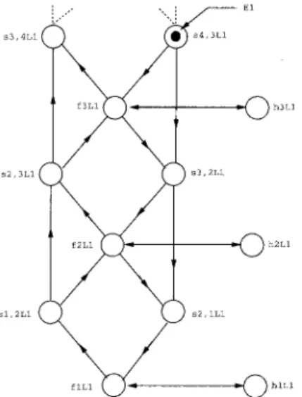
- The discrimination points are system configuration de- pendent. They are set by the user, to follow, for instance, the cabin trajectory inside a long blind zone, thus pre- venting the assignment algorithm from losing it in this zone. This type of information is not always necessary. Figure 2 represents one conceptual model of a possible cabin trajectory built using this restricted information.

This model is a graph, where vertices are called places, and links between places are called arcs. No discrimination points have been used in this example, but the following additional places have been introduced in order to represent two lift group states that are relevant for the assignment algorithm:

- Places h (home). When an elevator token enters these places, it means that it is parked. This happens when a lift has neither passengers nor orders to serve.

- Places c (cabin). When an elevator token enters these places, it means that the operation is transferred to the cabin, which is responsible to open doors and exit passengers.

In this model, in order to point out at each moment the current cabin position, a state marker, called token, is moved from place to place. Its trajectory in the graph reproduces the cabin trajectory in the speed/position state space. Each time the token El moves from one place to another, the assignment algorithm is informed and can update its internal information. Token motions from place to place take time. Durations depend on the real system features (cabin speed, acceleration, height between consecutive floors, etc.).

There is a graph for each particular real lift group. Even if each graph has its own number of vertices, durations and relationships between vertices, depending on the real system features, all such graphs contain exclusively the information types (place types) described above. This uniformity allows the development of a general assignment algorithm able to control any lift group.

The translation of the conceptual model into a computer program is related to the question: "who" controls E l ' s motions. There are at least two alternatives. In one approach, each visited place controls the token under normal operat- ing conditions, but a higher level place, called agent, takes over control of the token in emergency situations. In a sec- ond approach, the agent always controls the token El. In this paper, the second approach has been chosen. Figure 3 sketches the behavior of the agent, called LIFT, that controls the places of Fig. 2. The symbol # represents the level of a floor and @ the identification number of a lift. This function is associated to the LIFT agent, and is called enter function. The agent LIFT, is called the pilot of the places of the graph of Fig. 2. Section 5 describes how pilot places are set.

Figure 4 shows the complete conceptual model, built only with relevant information for the assignment algorithm. In this model, there are three types of agents: FLOOR, CABIN and LIFT. FLOOR is responsible to serve passengers at floors. It puts them in queues, where they wait for cabins. CABIN is responsible to manage cabin doors and passengers inside the cabin. Finally, LIFT is responsible to move cabins from floor to floor according to the ASSIGNMENT ALGORITHM orders and the cabin passenger destinations. The model uses

(3)

A. Stagno et al.: QOBJ modeling 111

A l g o r i t h m 1 LIFT entry function. /*

- the symbol # is the level of a floor and @ the identification number of a lift.

- dest_floor is the destination floor position of the elevator token. - curr_floor is the current floor position of the elevator token. - curr_class is the class of the current place of the token. - dest_class is the class of the destination place of the token.

- MOVE is the function that moves tokens from place to place. Its parameters are: the token to move, its destination place and the transition duration. */

case curt_class f#L@:

if dest_floor > curr_floor then

MOVE( El, s#,#+lL@, duration_f_to_s); else if dest_floor < curt_floor then

MOVE( El, s#,#-lL@, duration_f_to_s ); else

if dest_class = h then

MOVE( El, h#L@, duration_f_to_h ); else

MOVE( El, c#C@, duration_f_to_c ); s#,#+lL@:

if dest_floor > curr_floor then

MOVE( El, s#+l,#+2L@, duration_s_to_s ); else

MOVE( El, f#+lL@, duration_s_to_f ); s#,#-lL@:

if dest_floor < curr_floor then

MOVE( El, s#-l,#-2L@, duration_s_to_s ); else

MOVE( El, f#-lL@, duration_s_to_f ); end

Fig. 3. Part of LIFT entry function

three types of tokens: PASSENGER, ELEVATOR ( E l belongs to the ELEVATOR type) and ACTIVATOR. PASSENGER are sent by the trq[fic g e n e r a t o r I (not represented) to places t F @ (Travel request). Arrival of an ELEVATOR token on the place p F @ (Passenger) marks the end of the cabin door opening phase, whereupon PASSENGERS move from place t F @ to cabin q C @ (Queue). The ACTIVATOR token synchronizes the doors opening and the passenger entry operations. An- other case of synchronization between two agents is represented by the transition of token ELEVATOR between places f 3 L 1 and c 3 C 1 . When the cabin stops at a floor, the token E1 arrives in p l a c e f 3 L 1 . Control of this token is transferred from the LIFT to the CABIN, then cabin doors are opened and the ELEVATOR token is sent to the FLOOR through the transition c 3 C ! to p F 3 . Passengers can exit the cabin (transition from q C 1 to x F 3 ) or enter the cabin as mentioned above. In this scenario, the token E1 is transferred successively under the control of three agents and is used to synchronize their control activities.

3 E x i s t i n g s i m u l a t i o n p a r a d i g m s

The translation of the conceptual lift group model into a dynamic operating computer simulation program requires well- adapted simulation language features. The main modeling el- I The traffic generator is the module that creates passengers in a lift group simulation model.

ements of the lift group conceptual model to be represented in the computer program are the following:

- ELEVATOR tokens must be mobile and able to process information.

- PASSENGER tokens must be instantiable, mobile and able to process information.

- PASSENGER and ELEVATOR tokens must stay in places as long as necessary.

- Places and agents must be static and able to process information.

- Communication of active elements (elements that process information) must be visible.

- Operating control can be dynamically changed during simulation.

In short, the simulation language must provide at least a modeling element able to represent at the same time, mobile, active and instantiable elements, that allows the user to visualize communication of active element and that allows also a dynamic modification of operating control during simulation. Five representative existing simulation paradigms have been evaluated using the following modeling criteria:

- a c t i v e ~ p a s s i v e says whether an element is able to do processing or not,

- m o b i l e ~ s t a t i c says whether an element is able to move from queue to queue or not,

- i n s t a n t i a b l e says whether elements may be instantiated during simulation or only at start,

- a m o r p h o u s ~ r e a c t i v e says whether a queue allows a token to stay in it without processing or not,

- c o m m u n i c a t i o n v i s u a l i z a t i o n says whether communication between active elements is visible.

Table 1 summarizes the results of this comparison.

SIMAN V [7] models are sequences of b l o c k s that represent the processing to be applied to mobile elements, called p a r t s . Blocs are static, not instantiable and active elements (they can act on mobile and on static elements), while parts are mobile, instantiable and passive elements. Once a part enters a queue, its processing is started as soon as the down- stream resource (reserved using the SEIZE block) is free, thus making queues reactive.

QNAP2 [9] models are built using s t a t i o n s and c u s - t o m e r s . A station is composed of a queue and one or more servers. Stations are static, not instantiable, reactive and active, while customers are mobile, instantiable and passive. Customer services are described inside stations, using a pow- erful P a s c a L - l i k e language. Such a language allows the definition of a service that can be as complicated as necessary. Like SIMAN V and QNAP2, P e t r i n e t s , considered here as a simulation paradigm, are also composed of static, not instantiable and active elements, called p l a c e s , and of mobile, instantiable and passive elements, called t o k e n s .

SIMULA-67 [3] provides a different modeling approach. This language provides, through the s i m s e t package, the concepts of q u e u e s and c o r o u t i n e s necessary to build simulation programs. As SIMULA-67 is an object oriented language, all the modeling elements can be instantiated. Moreover, and on the contrary to the SIMAN V, QNAP2 and P e t r i n e t s approaches, SIMULA-67 queues are static, amorphous and passive, while coroutines are mobile and active.

(4)

1 PASSENGER . . . CABIN_ ELEVATOR - - 3CI ACTIVATOR qCl _/ ... ~[ ... . . . : :'::" / g3Cl LIFT

... /

iiiii

xF39

/

Fig. 4. Final lift group conceptual model

- - •

h3Ll S3,2LI - O h~L~

s2, ILl

: 9 h~L~

Table 1. Main features of existing simulation paradigms

A C T I V E P A S S I V E S T A T I C M O B I L E I N S T A N . Q U E U E C O M M .

SIMAN V queue part queue part part reactive visible

QNAP2 station c u s t o m e r station customer customer reactive visible

PETRI NETS place token place token token reactive visible SIMULA-67 coroutine queue queue coroutine q u e u e amorphous non visible

coroutine

This comparison shows that none of these simulation languages provides a modeling element having the features presented at the beginning of this section, i.e. with an amorphous queue, that can be instantiated during simulation, that allows the representation of both mobile and static and both active and passive elements, and that allows the visualization o f communication between active elements. Rather, QNAP2-

like approaches do not allow instantiation of mobile and active elements, while SlMULA-67-1ike approaches do not allow visualization of active elements communication. The next section will describe the most important features of the

qobj paradigm developed on the basis of these observations.

4 Qobj

modeling concept

There are two ideas at the origin of the qobj concept development. Firstly, even if the existing simulation paradigms make differences between mobile/static and active/passive elements, actually these elements can be included in a more general concept, which is mobile, active and instantiable. In- deed, static elements can be considered as mobile elements that do not move, passive elements as active elements that do not operate and non instantiable elements as simply instantiable elements that are not instantiated. This is in agreement with the French dictum saying qui peut le plus peut le moins!

Secondly, as queuing networks allow visualization o f active elements communication and object oriented approaches permit element instantiation, good model organization and element reutilization, the new concept must integrate these paradigms in some way.

Thanks to these observations and the integration of the best features of both queuing networks" and object approaches, it has been possible to build a unique concept that suppresses all above dichotomies, allows for a good organization o f the models and for a nice visualization of the communication o f the active elements.

It should be noted that the qobj paradigm is not just another object oriented simulation approach, comparable to languages like Simplex II (Eschenbacher [4]). Indeed, even though they bring interesting model organizing features, they do not suppress the limiting dichotomies discussed previ- ously, which can be a drawback when constructing complex and realistic models.

4.1 Main qobj attributes

A qobj is an object with the following elements: a unique

identifier, a class, a set o f attributes, a queue which can receive qobj, a parent (which is a qobj), a pilot (which is

a qobj too), an entry function, an exit function, a starting function, an ending function, a set of entering arcs and a set

of exiting arcs.

Class. Each qobj belongs to a class. The class defines the behavior and the attributes the qobj acquires when it is instantiated. There is a default class, called Q_QOBJ, from which users can derive new classes simply by defining or redefining the following parameters: the class name, the enter, the exit,

the starting, the ending and attributes functions (described below).

A t t r i b u t e s . There are system and user attributes. Attributes allow the association of information to qobj. They also provide a means of communication between qobj

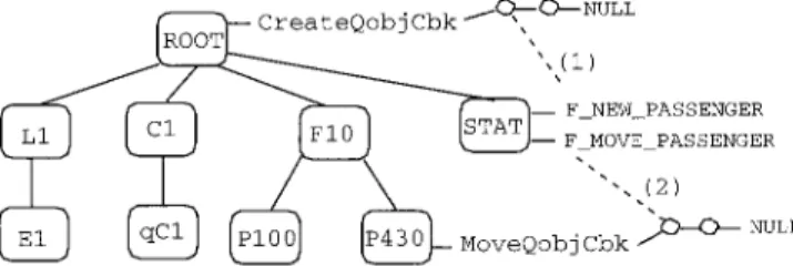
through the use o f callbacks. Indeed, each attribute has a list o f callback routines that are executed each time the value o f the attribute is modified. Figure 5 shows how two system callbacks MoveQobjCbk and CreateQobjCbk are used in order to follow the motion of PASSENGER type qobj. Each time a qobj is created, the user routines linked to the callback CreateQobjCbk are executed. To be informed of the creation of a new passenger, the qobj STAT must record its

(5)

A. Stagno et al.: QOBJ modeling

Creat eQobj

Cbk/IO~-O---NULL

C77

rsTA l--

PASSENGER

C

Fig. 5. Example of the use of the system callbacks MoveQobjCbk and CreateQobjCbk

113

(1) (2)

d e l a y

. . . ) ' " :: serv

Fig. 6. Qobj pilot entry and exit function activation after a MOVE

function F_NEW_PASSENGER in this list. Afterwards, in order to be informed of the motion of the created PASSENGER type

qobj,

it must record its function F_MOVE_PASSENGER in the callback

MoveQobjCbk

of the created passenger. Dur- ing simulation, new

qobj

can record themselves into a callback, whereas others may become unrecorded.

Queue.

Qobj

can communicate through execution o f callback routines, but their main feature is to be able to communicate through the exchange o f

qobj

which circulate into their queues. This allows the visualization of the communication between active elements.

Qobj

exchange allows modeling asynchronous (time delayed) communications. A

qobj

can send any

qobj

of the model to any other unless the

qobj

to be moved is already moving. The transition o f a

qobj

from one queue to another takes simulated time, even when the modeled duration of the transition is null.

Qobj

queues do not have a priority rule of type

fifo

or

lifo;

they are only places where tokens (token stands for "moving

qobj")

wait to be served. Ordering of

qobj

in a queue is the responsibility of the user. W h e n a token enters a queue, it is served by a service function (the

enter

function of the

pilot

(described below) of the queue). A t the end of the service, the token is either destroyed or moved to another queue or left in the queue. The latter possibility is allowed by the fact that

qobj

queues are amorphous.

As

qobj

can remain passively in a queue, their reactivation and synchronization with other

qobj

must be managed by the user. This is not the case in other queuing network discrete event simulators, Q N A P 2 o r SIMAN V, where synchronization and reactivation of entities is automatically managed by the simulator. The explicit management o f synchronization and reactivation can be annoying in some cases. However, it allows more flexibility when the control of the operation of the model is complicated, for example when the model represents a complex system.

Parent. W h e n a

qobj

is created it is not necessarily inserted into a queue. It can "float" anywhere in the model, without

a parent.

The first time it is moved into a queue, it acquires a parent. The parent of a

qobj

is simply the owner o f the queue to which it is attached at a given moment. The parent of a

qobj

changes when the

qobj

moves from one queue to another. During transitions, a token carries with it all

qobj

whose father it is.

Pilot, entry function and exit function. Consider Fig. 6. W h e n token D moves from

qobj 13

to

qobj C,

several operations are realized. First, the

exit function 'fexit"

of pilot

P(B)

of the origin

qobj B

of the token is executed. There- after, the

entry function 'renter"

o f pilot

P(B)

of the desti-

nation place C (place stands for

"qobj

receiving tokens") of the token is executed. Token processing is done inside these functions

(entry function

and

exit function). Entry functions

control token routing, while

exit functions

update internal data of their associated

pilot.

The

exit function

is necessary to keep internal integrity of pilots, because any

qobj

can move any other

qobj.

Indeed, if a

qobj

different from the pilot o f a queue moves a token out of that queue, the pilot must be informed in order to update his internal data. This information is given b y the

exit function.

Such type of function is unnecessary when

qobj

are moved only by the pilots of the queues.

The pilot of a

qobj

can be either the

qobj

itself or another

qobj

of the model. This type of control allows centralizing or distribuing services inside the model according to the operating conditions. We can imagine two extreme configu- rations: in the first, all the queues o f the model are m a n a g e d by only one

qobj

and in the second, each

qobj

manages its own queue. In the first case, the system is totally

centralized:

there is only one pilot for all the qobj, while in the second case, the system is completely

distributed:

each

qobj

being its own pilot.

The pilot of a

qobj

can be changed during the simulation, thus making it possible to delegate control of the system to the lowest level

qobj

when the system operates normally and to centralize it in case o f an emergency (fire, breakdown, etc.). The pilot mechanism introduces a new form of organization into the models based on the centralization/distribution of the control.

Starting function and ending function. At the beginning o f simulation

qobj

may need to initialize their internal data. For that purpose, a

starting function

is associated to each

qobj.

Likewise

an ending function

is associated to each

qobj

to update its internal data at the end o f a simulation run.

Starting functions

o f each

qobj

are executed before the first token is moved. Similarly, the simulator executes the

ending functions

at the end o f each simulation run. As

qobj

are not ordered in queues, it is impossible to know their starting or ending order. If a precise order is needed, it must be coded in the model. In this case, an initializing token is created by one o f the

qobj

o f the model and is m o v e d from

qobj

to

qobj

in the desired order.

A r e s . Arcs are elements introduced to ease construction o f simulation models and to serve as information support, as in Fig. 4.

Arcs

belong to classes, have attributes, but do not have functions, indeed, processing is only accomplished inside

qobj

service functions. Attributes are values or functions which, for instance, return a transition duration, or informa-

(6)

tion on tokens that can do the transition. For a

qobj,

the set of its entering and exiting arcs represents information that can be used in its

enter

and

exit

functions.

4.2 Main qobj concept features

The particular structure and behavior of the

qobj

concept confer several interesting features to it. Some are inherited from the

object

and

queuing network

paradigms, while others are completely original.

Qobj

concept polyvalency. In

qobj

simulation models there is no difference between dynamic and static elements. There are only

qobj,

that can be both mobile or static depending on their use. This feature is called the

qobj

concept polyvalency. The

qobj

modeling approach goes further, as it is op- posed to one of the current trends, supported by the graphic simulators, which recommend the development of specialized modeling concepts such as machines, trucks, pallets, conveyors, etc. It is easy to use these elements with corresponding systems, but as they are specialized, they can only be used for these systems and not for others. On the contrary,

qobj

is a general modeling concept, that can be used for a large number of systems.

Organization forms in the

qobj

models. In

qobj

models there are three types of organization:

hierarchies',

by parent links;

networks,

by

qobj

motions; and

centraliza-

tion~decentralization

of control, by the pilot and the service functions mechanism.

Hierarchical organization.

The

qobj

concept polyvalency allows the design of hierarchical models with many different levels. Indeed, since there is only one type of element in the model (the

qobj)

and since each

qobj

has a queue, any

qobj

can be the son of any other

qobj.

With alternative simulation~ approaches, that have only one hierarchical level: queues that control tokens, it is harder to model hierarchical systems.

Queuing network organization. Qobj

moving between queues can describe flow of both information and materials. Mod- els can be considered as networks whose nodes are the

qobj

and whose links are the transitions from one

qobj

to another. The

qobj

of a given class generally visit a subset of

qobj

of the model. Linking together two consecutive

qobj

on such a path results in a network representing a

process.

This form of organization comes from discrete event simulation queuing network.

Centralization~distribution organization.

This form of organization comes from

qobj

mechanism based on the pilot and the service functions

(entry

and

exit

function). This mechanism allows the separation of the representation of the system from its control. Inside the models, it is possible to modify the distribution of the control simply by modifying the pilot and the service functions of the

qobj

during the simulation. This form of organization does not exist in other queuing networks approaches. Indeed, in queuing networks, token motions depend on implicit rules of the network elements (servers, resources, semaphores, etc.), which block or release tokens according to their intrinsic simulation behavior. The user gathers these elements and verifies that the

resulting model produces the correct behavior. The control of the tokens is completely (in S~MAN V) or partially (in QNAP2) contained in the network, as well as in Petri nets where token transitions depend only on the state of the network and on its structure. The implicit motion of the tokens, as well as the dichotomies introduced between mobile/static and active/passive elements, are a help to the user, but only until the model becomes too complex, at which time this aspect turns into an obstacle hard to surmount.

Types of communication in

qobj

models. There are two types of communication in

qobj

models: one is based on the exchanges of

qobj

and the other on the execution of callback routines.

Communication based on qobj exchange.

This type of communication, which comes from the queuing network approach, has the nice property to be visible.

Qobj

motion is particularly well adapted for asynchronous communication description.

Communication by callbacks.

This type of communication allows the description of synchronous exchanges of information. Compared to the

qobj

exchanges, this type of communication is less expensive in execution time, because it consists only of direct routine calls without using the scheduler which controls the simulated time.

Integration of paradigms. The

qobj

concept does not ex- clude other types of paradigms as for instance Petri nets or neural nets, rather it integrates them. Indeed, these approaches can be used for the implementation of the

qobj

service functions. This property, coming from the object origin, allows the use of the most appropriate formalism there where it is needed.

4.3 Qobj modeling rules

Basically, the

qobj

modeling process consists in identifying the elements of the system to be represented by

qobj.

The

qobj

modeling rules come directly from the features of the

qobj.

As a

qobj

can be either static or mobile and either active or passive, it can represent: a

processing element

of the system, a

mobile element, a state element, a state marker,

or a

communication element.

A processing element

is an element that transforms other elements, computes, optimizes, etc. All these operations can be realized by

entry

and

exit

functions of each

qobj.

In a lift group, examples of processing elements are assignment algorithms, logical modules that generate passengers, statistics modules, etc.

A state element

represents either a particular state of the system (out of order, working, waiting for furniture, ...), or an event that provokes the start of an activity (arrival of a cabin at a floor .... ), or finally an activity of a more complex process (painting, machine operating a part .... ). In the model, where

state elements

are represented by

qobj,

state and process models can be nicely visualized. A token (another

qobj),

which moves from one

state-qobj

to another, is sufficient to mark the current state of the model and its route is sufficient to allow process visualization. Such a token is called

state marker.

Section 2 will provide an example of a state marker used in lift group models.

(7)

A. Stagno et al.: QOBJ m o d e l i n g 115

A communication element

is a message exchanged between two processing elements, it can serve to send information, or to synchronize their activity. A

communication

element

can be also a

state marker,

in which case it gives the state o f the model at each moment.

It should be noted that the role o f a

qobj

is not fixed, but it can vary during the simulation. For instance, at some given moment it can be a processing element and at another, a message. A passenger can be thought of as a communication element between the

floor

and the

cabin,

but also as a processing element when it receives orders from the system that indicate him which cabin to enter. We can also notice that a

qobj

can be a processing element at a given m o m e n t and a state marker at others. For instance, as described in Sect. 2, a

selector

is a lift engine state represented by a

qobj,

but it is also a processing element which moves the

elevator

tokens.

5 QOBJIGEOS s i m u l a t o r

This section describes how the conceptual lift group simulation model, described in Sect. 2, has been translated in a computer program using the general purpose QOBJ-GEOS simulator which is based on the

qobj

paradigm. The first QOBJ-GEOS modeling step consists in defining a

qobj

class library covering the domain of interest. Then, in any order, the following operations must be realized: build a particular instance o f the model, define the statistics and describe the experiments to run.

5.1 Domain-specific qobj library

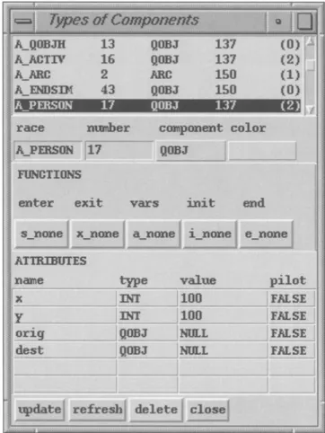
As the QOBJ-GEOS is a general purpose simulator, the first modeling stage consists in the definition o f a domain-specific lift group

qobj

library. New

qobj

classes are built using the w i n d o w o f Fig. 7. For that, the user must provide the class name, the type o f the new class

(qobj

or

arc'),

the color, the class parameters and the

qobj

class service functions. These functions are written in a c + +-like programming language developed specifically for the QOBJ-GEOS simulator. All the

qobj

o f a same class have the same parameters, but can have different parameter values. Parameter values are set during the model building stage (Sect. 5.3).

5.2 Statistics definition

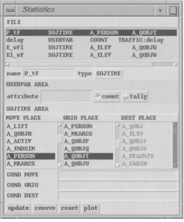
QOBJ-GEOS allows the definition o f three types o f statistics. These statistics are defined in terms o f

qobj

and their parameters:

- SOJTIME: measures the time spent by a type of

qobj

in

a qobj

of another subset. For instance, it is possible to measure passenger waiting time in a lift group by measuring the sojourn time o f all the

qobj

o f type PERSON in any

qobj

o f type A_PLACEQ (place

qC@).

- TRAVTIME: measures the time necessary for a given

qobj

(belonging to a user-defined subset) to move from a

qobj

(of a second subset) to another

qobj

(of a third subset). For instance, this type o f statistic can be used to measure

Fig. 7. Class definition w i n d o w

the time required for a

qobj

of type ELEVATOR to go from a

qobj

A_PLACEP to a

qobj

A_PLACEP (place

pF#),

i.e. from floor to floor.

- USERDATA: measures the successive value changes o f

qobj

and

arc

parameters. F o r instance, this type o f staffs- tic can be used tc~ measure queue levels over time. It is possible to measure value changes only, or value changes over time (integrals).

Figure 8 shows the statistics definition window. This example refers to a SOJTIME type statistics definition, used to measure waiting time o f passengers at a floor. It is possible to display several curves in the same w i n d o w and plot discrete observations and mean continuous curves. Figure 9 contains two curves: mean passenger waiting time and their mean inter-arrival time. This window also contains the indi- vidual observations o f each statistic. For each statistic, the mean value, the confidence interval at 95% and the number o f observation can be obtained (Fig. 10). It is also possible to get the cumulative empirical distribution and the transient curve for each statistic.

5.3 Qobj model building

Model building consists in picking up necessary elements from the class library and parameterizing them (setting attributes values) according to model features. These operations can be done either manually using a mouse, or by program when models are too large. For lift group models,

(8)

Fig. 10. Passenger waiting time (P_tF) statistics summary

Fig. 11. Initialization of main level

qobj

Fig. 8. Statistic definition window.

Fig. 9. Passenger waiting time and inter-arrival time (observations and mean curves)

Fig. 12. GROUP parameters window

both m e t h o d s have b e e n used. First, m a i n level

qobj

have b e e n m a n u a l l y created (Fig. 11), then service functions of these

qobj

have created their subnets.

T h e GROUP s u b n e t is built in four steps. First of all, its

initfunction

m a k e s instances of FLOOR, LIFT a n d CABIN

qobj

according to

floors

a n d

lifts'

variables of the

qobj

GROUP and puts them in its queue.

Floors

a n d

lifts'

variable values are interactively set b y the user through the GROUP p a r a m e t e r w i n d o w (Fig. 12).

T h e n the GROUP sends a A_MKQOBJ

qobj

to the first LIFT. W h e n a LIFT receives such a

qobj,

it creates its o w n subnet (Fig. 14), then the

qobj

A_MKQOBJ is m o v e d to the next lift, then to each CABIN and finally to each FLOOR, until all the

qobj

have built their o w n subnet. T h e last operation consists in s e n d i n g a

qobj

A MKARCS, following the same circuit, w h i c h indicates to the LIFT, CABIN a n d FLOOR to create the links b e t w e e n the

qobj

in their queue.

(9)

Fig. 13. GROUP initialization subnet

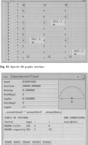
Fig. 15. Specific lift graphic interface

Fig. 14. Part of the model hierarchy

5.4 Animation

The QOBJ-GEOS simulator allows visualizing of

qobj

motion from queue to queue. This form o f visualization corresponds to the

qobj

motion from window to window, as a window can always be associated to a

qobj

queue contents. More- over, the user is also allowed to include an external graphics interface written in C++ (Stroustrup [11]) and O S F Motif. Figure 15 shows such an interface developed for the lift group models. In this figure the interface has been instantiated for a lift group composed of 10 floors and 3 lifts. The third column represents floor buttons state (pushed or re- leased). The fourth, the seventh and the tenth columns show the first, the second and the third cabin buttons state (passenger destinations) respectively. The fifth, the eight and the eleventh columns show the assignment orders of these cabins. The sixth, the ninth and the twelfth columns show the position of these cabins.

5.5 Experiment design

Two types of experiments (Jain [5]) can be defined in QOBJ- GEOS. The first, called 1 k for

simple design,

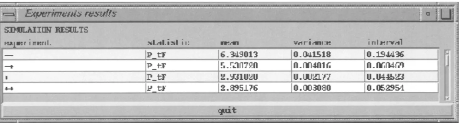
consists in ex- ecuting several runs, each one differing from the initial run only by one model parameter value. The second type of experiments, called 2 k, consists in running factorial experiments. In this type of experiments, the user gives several

Fig.

16. 2 k experimental plan

parameters and defines for each parameter a m i n i m u m and a m a x i m u m value. A t the beginning of the simulation, the simulator computes the 2 k (where k represents the number of parameters) experiments and runs them. Figure 16 contains a 2 ~ experiment definition, where two parameters of the

qobj

GROUP have been selected:

lifts

and

capacity.

Results of the four corresponding runs are illustrated in Fig. 17. These results may be used in a regression meta-model computation that can be used for optimization (Kelton & Law [6]).

6 Assignment algorithm

This section shows how the

meta-model

o f Fig. 4 is used by the

assignment algorithm

in order to compute its assignments. It is also shown how the graphical user interface of the QOBJ-GEOS simulator has been helpful for the assignment algorithm validation. The algorithm presented in this section, being mainly developed to validate the simulation model of lift groups, it has the advantage to be very simple.

(10)

Fig. 17. Results related to 2 k experiments defined in Fig. 16

6.1 Communication between the algorithm and the model

During simulation, the assignment algorithm and the lift group model exchange the following types of information:

- The model sends to the algorithm important trigger events that take place in the model.

- The algorithm reads the model state information for com- puting assignments.

- The algorithm sends orders to the cabins at the end of computations.

These types of information can be expressed within a for- mal communication language based on the state elements represented in the model of Fig. 4.

S t a r t i n g events. The assignment algorithm is informed by its callback routines associated either to the system callback

moveQObjCbk of each token elevator, or to the user callback

pushButtonCbk of each place tF. These routines are executed by the simulator each time a token elevator has m o v e d and each time a floor button state has changed. Information on token elevator position is useful to detect the instants when the cabin has no more destinations to serve, i.e. when the associated elevator token enters one of the places wF or hL

o f the model. Each time the algorithm is called, it computes again all cabin destinations. In some lift groups, it is not only necessary to follow cabin motions but passenger motions too. Some example o f starting events are given below:

<date> E1 pF3 Elevator E1 is in pF3: waiting for passengers boarding.

<date> E2 wF5 Elevator E2 is in wF5: cabin C2 parked under floor F5 control.

<date> E3 h9L3 Elevator E3 is in h9L3: cabin C2 parked under algorithm control.

<date> P1 tF1 Passenger P1 is in tFl: waiting at floor FI. <date> P3 qC4 Passenger P3 is in qC4: waiting in cabin C4. <date> P9 xF8 Passenger P9 is in xFg: exiting the system. Information on floors button state changes are generated by user pushButtonCbk callback

- when a token elevator leaves a place pF (end of passenger boarding).

- or when a new passenger arrives at a floor and pushes a button. The button in a given direction can be pushed only by the first passenger.

In the first case, the algorithm checks whether the leaving cabin has served a floor call, whereas in the second case the

algorithm is informed o f a new floor call to serve. Some examples, valid for a floor with two buttons: one to go up and another to go down, are given below:

<date> tFl 0P There are no waiting passengers at floor FI.

<date> tF3 *P {up} There are waiting passengers to go up, at floor F3.

<date> tF5 *P (up} {down} There are waiting passengers to go up and down, at floor F5. State information. When the algorithm computes the assignments, it needs some additional information concerning, for instance, the motion direction of the cabins, their serving direction, their position, the number of passengers they contain, etc. The assignment algorithm reads this information directly in the model, by examining attributes associated to the qobj and by reading their queues. S o m e example are given below:

! <date> qC1 0P : Cabin C1 is empty.

! <date> qC2 4P {xF4} {xF9} : Four passengers in cabin C2; floors F4 and F9 are selected. In a real system, with two buttons at each floor, the number of passengers is approximately only obtained with a balance in each cabin. In a simulation model, this information can be obtained accurately, simply by reading the qobj contained in the cabin queues.

O r d e r s . The assignment algorithm sends the cabins their new destinations by the means of orders. An order is composed o f an elevator identifier and one or many destinations. A destination is one of the places of the model represented in Fig. 4 and sometimes a serving direction. There are three types o f orders: clear orders, service orders and park or- ders. Clear orders allow cancelling of previous orders sent to a cabin. Service orders tell the cabins to serve a particular floor call. Finally, park orders tell the cabins to get parked. Some examples o f orders are given in the array below:

!! <date> E1 Clear previous orders for cabin C1.

!! <date> E1 pF3 (down} Cabin C1 must serve serving direction down of place pF3. !! <date> E1 wF1 Cabin CI must park under con-

trol of floor FI.

!! <date> E1 h2L1 Cabin C1 must park under control of the assignment algorithm at floor F2.

(11)

6.2 Assignment policy

Assignments of floor calls to cabins are computed using heuristic rules, initially based on common sense and further validated by (simulation) experiments in order to improve their efficiency. The following terms are necessary to understand the assignment algorithm.

- A cabin serving direction indicates the floor buttons (uP o r D O W N ) it serves.

- A cabin is parked if its associated

elevator

token is in place

wF

or in place

hL.

- A cabin is not empty if it contains at least one passenger. - A cabin is served if it is p a r k e d and it receives a new

destination, or if it is not empty.

- Assume that the floors of a building are numbered in an increasing way from the bottom to the top. This number is called floor position.

- A cabin is above (resp. below) a floor, if the cabin goes up and the floor position is g r e a t e r (resp. smaller) than the cabin position, or if the cabin goes down and the floor position is smaller (resp. greater) than the cabin position.

The assignment algorithm (algorithm 2) is composed of three main rules, chosen and organized in order to assign all the current floor calls to the maximum number of cabins.

Algorithm 2 Assignment algorithm.

lif there are floor calls to serve then

2 Assign floor calls to parked cabins, according to their serving direction. 3 Assign floor calls to non empty cabins with the same serving direction. 4 Assign remaining floor calls to not yet served cabins, according to their

serving direction.

5end

Fig. 18. Assignment algorithm

The objective of the step 2 of algorithm 2, detailed in the algorithm 3, is to distribute the floor calls among a maximum number of cabins, by serving parked cabins first. As parked cabins do not have destinations, it is possible to assign them floor calls in any serving direction. Meanwhile, in order to minimize the cabins travel, floor calls assigned to a parked cabin all have the same serving direction and are all above the cabin or all below it. After this step, cabins with at least one destination are considered as served and are ignored in the next two steps of algorithm 2. In the same way, when a floor call has been attributed to a cabin, it is marked and it cannot be reassigned in the second part of the algorithm (see Fig. 19).

The objective of the step 3 of algorithm 2, detailed in algorithm 4, is to serve non empty cabins just after parked cabins. As their serving direction is fixed by the serving direction of the passengers they contain, the assignment algorithm gives them only floor calls above with the same direction as their serving direction. The aim of this policy is to fill cabins that still contain passengers. But, as this policy does not take into account the capacity of the cabins, it can happen that during their travel they become full and cannot serve floor calls assigned to them by the algorithm. At the end of this step, all cabins that already contain passengers are considered as served, even if they have not received

Algorithm 3 Floor calls assignment to parked cabins.

for each cabin do if parked then

Mark as served the current cabin.

servdir = serving direction of the cabin.

if servdir = NONE then servdir = UP.

Assign to the cabin all the floor calls above, with the same serving direction than servdir.

if the number of assignments = 0 then

Assign to the cabin all the floor calls above with the opposite serving direction than servdir.

if the number of assignments = 0 then

if servdir = UP then servdir = DOWN else servdir = UP. Assign to the cabin all the floor calls below with a same serving direction than servdir.

if the number of assignments = 0 then

Assign to the cabin all the floor calls below with an opposite serving direction than servdir.

end end

Send orders to the cabin.

end

Fig. 19. Floor calls assignment to parked cabins

new destinations. These cabins are ignored in the following phase.

Algorithm 4 Floor calls assignment to non empty cabins.

for each cabin do if not empty then

Mark the current cabin, as being served.

Assign it all above floor calls with the same direction than its serving direction.

end end

Fig. 20. Floor calls assignment to non empty cabins

The objective of the step 4 of algorithm 2 is to assign floor calls to the cabins that are not yet served. This step ends only when all cabins become served, i.e. when they have received at least one new destination. Assignment of floor calls to each non served cabin (algorithm 5) consists in searching a serving direction for which there is at least one possible destination for the cabin. If such a serving direction is found, then all destinations with this serving direction are assigned to the cabin. This process is repeated until all cabins are served. After each iteration, all floor calls are unmarked and can be reassigned to cabins that have no destinations yet (see Fig. 21).

6.3 Traffic in lift groups

In lift simulation models, the general passenger traffic model is defined using four parameters: traffic intensity, given in number of passengers per second, and the percentages of

up-

peak, down-peak

and

inter-floor

passengers, which represent respectively the proportion of passengers that go from the main floor (generally the first floor), to the other floors in the building, the proportion of passengers that go from all the floors in the building, except the main floor, to the main floor, and finally, the proportion of passengers that go from any floor, except the main floor, to any other floor, except the main floor. The percentages

up-peak, down-peak

and

inter-

floor are

linked by the formulas given in the left column

(12)

A l g o r i t h m 5 Floor calls assignment to remaining cabins.

f o r each cabin d o i f not served then

servdir = serving direction of the cabin.

i f servdir = NONE then servdir = UP.

Assign to the cabin all the floor calls with the same direction as servdir.

if the number of assignment equal 0 then Assign to the cabin all the floor calls with the opposite direction of servdir.

if the number of assignment equal 0 then

i f servdir = UP then servdir = DOWN else servdir = UP. Assign the cabin all the floor calls

with the same direction as servdir.

i f the number of assignment equal 0 then Assign to the cabin all the floor calls with the opposite direction of servdir.

end end

Send orders to the cabin.

Mark the current cabin as being served. end

Unmark all the floor calls, even if they have been assigned.

e n d

Fig. 21. Floor call assignment to remaining cabins

50 f$ v O] 03 m t~ ! i f \ i / '%

i

. - - - r ; 2 y "

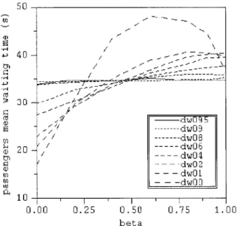
3 0 --[- - " - /" ~ "' j ,.,fS ''~/" d w 0 9 5 ,. . . . . d w 0 9 / / / . . . dw08 2 0 ~ / .4 1 0 0.00 0.25 . . . duO 6 . . . . dwO ~1 ... d w 0 2 - - - d w O 1 - - - d w O :3 0 . 5 0 0 . 7 5 1.00 b e t a

Fig. 22. Passengers mean waiting time as a function of/3 and down-peak

below, which are equivalent to those expressed only with two variables: /3 and

down-peak,

in the right column. The latter traffic formulation is used in point 6.4.

0<_3_<1 0 < up-peak < 1 0 < down-peak <_ 1

0 _< down-peak <_ up-peak up-peak = ( I -/3)(1 - down-peak) inter[toor = 1 up-peak-down- inter[toor =/3(1 - down-peak)

peak

6.4 Assignment algorithm performance analysis

Several operating conditions have been tried in order to evaluate the performances of the assignment algorithm 2. Ex- periments have consisted in varying the parameters /3 and

down-peak

and in measuring the influence of these parameters on the mean passenger waiting time. They have been realized using a building with l0 floors and 3 cabins with a capacity of 10 passengers each, no passengers in the building at the beginning of the simulation. Traffic intensity was always equal to 1 passenger each 6.66 seconds. Each configuration has been simulated 5 times (5 replications) over 50000 units of time (seconds). Results are represented in Fig. 22. Each point is a mean of five measures.

For

down-peak

equal 0, mean passenger waiting time is at its minimum when/3 is equal to 0. Then it grows until/3 is equal to 0.6 and decreases until/3 is equal to 1.0. For

down-

peak

taken in the interval [0.1...0.6], the mean passenger

waiting time grows in a monotonic way in function of/3. Finally, for

down-peak

bigger than 0.6, the mean passenger waiting time is more or less constant, independently of the value of/3.

Traffic 0%

down-peak.

Consider the case where

down-peak

is equal to O. W h e n / 3 is equal to O, i.e. when traffic is 100%

up-peak,

cabins start to load passengers at the first floor and go up the building. During their travel they unload passengers and when the last passenger has exited they return to

the main floor where the cycle starts again. It can be considered that, when the system is stable, i.e. when queues do not explode, this traffic results in the smallest mean passenger waiting time, as shown in Fig. 22.

When /3 grows, the part of the

interfloor

traffic grows too. In this case, cabins cannot come back to the main floor as quickly as when /3 is equal to 0, because they have to serve

inter-floor

passengers. Moreover, the larger the

inter-

floor

traffic becomes, the less frequently cabins come back

to the main floor, with the consequence that the passengers' mean waiting time becomes larger and larger, because a ma- jority of passengers have to wait for a minority to be served. It is for/3 about equal to 0.6 (for the experienced system) that

inter-floor

passengers most disturb the assignment algorithm performance. W h e n / 3 is greater than this value, mean passenger waiting time decreases again, and for/3 equal to 1.0, it reaches the same value as that obtained with a 100%

down-peak

traffic.

Such a performance has been first imputed to the

inter-

floor

passengers perturbation. However, after analyzing the

behavior of the cabins with the graphical simulator, the influence of parasite cycling phenomena affecting empty cabins was identified as having a major influence. This cycling phe- nomenon was caused by the assignment algorithm decision rules based on the

serving direction.

Figure 23 explains with an example cycling problems discussed above. In part (1) of the figure, the cabin waits at one floor. In part (2), it receives a new order to serve the

up

floor call at floor 1. Then, it mod- ifies its serving direction, which becomes

{up},

and starts to move to floor 1. Before arriving at its destination floor, a new floor call arrives from above (part (3)). Then, the algorithm again computes the assignments and according to its rules, gives the cabin an order to serve the new floor call. The consequence is that the cabin changes its serving direction, which becomes

{down},

and inverts its moving direction which becomes

{up}

(part (4)). If alternately floor calls above and below an empty cabin arrive, the cabin can

(13)

A. Stagno et al.: QOBJ modeling 121 n u m b e r of passengers in the cabin

\

serving direction \ cabin floor call

D

floor call assigned to the cabin

moving direction

I A opl

2'

/

m

V

,ik

D

IJoPI

/x

7q

_{Fig. 23. Cycling problems with the algo-}

rithm 2

begin to cycle, with the consequence that passengers have to wait at floors to be served and the mean passenger waiting time becomes larger and larger.

This problem only concerns empty cabins and that only when the percentage of

inter-floor

traffic is sufficiently high. In this case, each new floor call can invalidate previous assignments. This type of degeneracy does not affect the mean passenger waiting time when traffic is 100%

inter-floor,

for two reasons: firstly, because there are no passengers waiting at the first floor, so there are no passengers that can be ignored, and secondly because the passengers mean inter- arrival time (parameter

mean)

is sufficiently high that the cabin cannot cycle too much. Indeed, when there are enough floor calls, the cabin is in some way obliged to serve at least one of them, and once it is no longer empty, it can no longer cycle.

Down-peak

t r a f f i c c o m p r i s e d b e t w e e n 0 . 1 a n d 0 . 6 . The degeneracy observed for

down-peak

equal to 0, tends to dis- appear as the percentage of the

down-peak

traffic increases. Indeed, when this percentage becomes different from 0, the probability that a cabin loads a

down-peak

passenger becomes non zero. When such a passenger is in a cabin, the cabin must go to the first floor and waiting passengers there are served. In this case, the risk of degeneracy decreases when the

down-peak

percentage increases. This analysis is confirmed by results illustrated in Fig. 22.

Down-peak

t r a f f i c a b o v e 0.6. When the percentage

down-peak

of traffic rises beyond a certain value (here 0.6), the mass of these passengers is large enough to influence the mean passenger waiting time. This is the reason why this measure does not depend on the/3 parameter. To sum- marize, it can be said that the assignment algorithm 2 works correctly as long as there is a small percentage of

down-

peak

traffic in the system. Otherwise, its performance tend to degenerate.

6.5 Corrected assignment algorithm

In order to correct the problems of assignment algorithm 2, algorithms 3 and 5 have been modified in such a way that decisions are no longer based on the

moving direction

but on the

serving direction

of the cabins (algorithm 6). Thus, the new algorithm is simply obtained by replacing the serving direction

servdir

by the moving direction

movedir

every- where in the rules 3 and 5.

50 4--) O~ .,,I -e4 o l @ r n o~ 43 36 29 22 ~ / / 15 0 . 0 " - - ' ; /

... d~59

, _ ~, i/ ... d ~ 3 8 / / ; / - . . . . d ~ 3 6 , / / - - - d ~ r s / ... d ~ 3 2 - - - d ~ 3 i - - - d ~ O O I ' I ' I ' i 0 . 2 0 . 4 0 . 6 0 . 8 }>~ta 1 . 0

Fig. 24. Passengers mean waiting time as a function of/3 and down-peak

A l g o r i t h m 6 Corrected assignment algorithm. l i f there are floor calls to serve t h e n

2 Assign floor calls to the parked cabins, with respect to their m o v i n g d i r e c t i o n .

3 Assign floor calls to not empty cabins with the same s e r v i n g d i r e c t i o n .

4 Assign floor calls to remaining cabins, with respect to their m o v i n g d i r e c t i o n .

5 e n d

in order to verify the positive effects of the previous modifications, the experiments, described at the point 6.4 have been rerun using the corrected algorithm. The results (Fig. 24) show that the errors have been corrected.

When the percentage of

down-peak

is less than or equal to 60%, the mean passenger waiting time of the new algorithm is less than that obtained with the old one. In this case, as cabins do not cycle with the corrected algorithm, passengers can be served more rapidly. When the percentage of

down-peak

is greater or equal to 80%, both algorithms per- form in a similar way. There are two reasons that explain this result. First, for this percentage of

down-peak,

the first algorithm was not affected by the cabins cycling problems,