Export Diversification:What's behind the Hump?

HAL Id: halshs-00556999

https://halshs.archives-ouvertes.fr/halshs-00556999

Preprint submitted on 18 Jan 2011

HAL is a multi-disciplinary open access archive for the deposit and dissemination of sci-entific research documents, whether they are pub-lished or not. The documents may come from teaching and research institutions in France or abroad, or from public or private research centers.

L’archive ouverte pluridisciplinaire HAL, est destinée au dépôt et à la diffusion de documents scientifiques de niveau recherche, publiés ou non, émanant des établissements d’enseignement et de recherche français ou étrangers, des laboratoires publics ou privés.

To cite this version:

Olivier Cadot, Céline Carrere, Vanessa Strauss-Khan. Export Diversification:What’s behind the Hump?. 2011. �halshs-00556999�

1

Document de travail de la série Etudes et Documents

E 2009.34

Export Diversification:

What’s behind the Hump?

*

Revised version November 2009 Olivier Cadot∗ Céline Carrère+ Vanessa Strauss-Kahn§ *

Research on this paper was supported by a grant from the Interamerican Development Bank and by Switzerland’s Fonds National pour la Recherche Scientifique. Special thanks go to Julien Gourdon for attracting our attention to key data and estimation issues. Without implicating them, we would also like to thank Marius Brülhart, Antoni Estevadeordal, Christopher Grigoriou, Jaime de Melo, Marcelo Olarreaga, Christian Volpe, two anonymous referees and the editor for useful comments.

∗ _{The World Bank, HEC Lausanne, CERDI, CEPR and CEPREMAP.} + _{CERDI-CNRS, Université d’Auvergne.}

§

2

Abstract

The paper explores the evolution of export diversification patterns along the economic development path. Using a large database with 156 countries over 19 years at the HS6 level of disaggregation (4’991 product lines) we look for action at the “intensive” and “extensive” margins (diversification of export values among active product lines and by addition of new product lines respectively) using various export concentration indices and the number of active export lines. We also look at new product introduction as an indicator of “export-entrepreneurship”. We find a hump-shaped pattern of export diversification similar to what Imbs and Wacziarg (2003) found for production and employment. Diversification and subsequent re-concentration take place mostly along the extensive margin, although the intensive margin follows the same pattern. This hump-shaped pattern is consistent with the conjecture that countries travel across diversification cones, as discussed in Schott (2003, 2004) and Xiang (2007).

Keywords: Export diversification, International trade JEL classification codes: F1, O11

3

1. Introduction

Why should export diversification be taken as a policy objective per se? There are two reasons why it should not. First, according to Ricardo, countries should specialize, not diversify. Second, the Heckscher-Ohlin model implies that export patterns are largely determined by

endowments; so if anything we should worry about factor accumulation, not diversification. Yet, export diversification is a constant

preoccupation of policymakers in developing countries. As de Ferranti et al. (2002) note, “[a] recurrent preoccupation of [Latin American]

policymakers is that their natural riches produce a highly concentrated structure of export revenues, which then leads to economic volatility and lower growth” (p. 38).

The notion that export patterns are fully determined by endowments is of course naïve. The relationship between endowments, trade, and growth is a complex and imperfectly-understood one. Intra-industry trade models have shown long ago that many factors other than endowments, including market failures and policies, can affect trade patterns. More recently, Hausmann, Hwang and Rodrik (2007) argued that export patterns can display path dependence in the presence of externalities.

Policy concerns about a linkage between the concentration of exports on primary products and deteriorating terms of trade, income volatility and, ultimately, low growth, goes back to the work of Prebisch (1950) and Singer (1950). Subsequent work (e.g., Neary and van Wijnbergen (1986), Gelb (1988), Auty (1990), or Sachs and Warner (1999)) showed a robustly negative correlation between dependence on primary products and future growth, a finding called the “natural-resource curse”.1 _The

negative correlation between natural resources and growth was however questioned by, among others, Brunnschweiler (2008) and

Brunnschweiler and Bulte (2008), who argued that regressing growth on the share of primary products in exports or GDP suffered from fatal endogeneity problems.

1 _{The Prebisch-Singer hypothesis implies that low growth is caused by dependence}

on primary products, not necessarily by concentration per se. However, preliminary findings by Dutt, Mihov and van Zandt (2008) suggest that

diversification does accelerate future growth, especially when it is accompanied by convergence toward the U.S.’s pattern of exports.

4

While the relationship between endowments, trade, and growth has remained a controversial issue, how export patterns vary across time and countries has become a subject of intense descriptive analysis in recent years. Several papers (e.g., Evenett and Venables (2002),

Hummels and Klenow (2005), Kehoe and Ruhl (2006) or Brenton and Newfarmer (2007)) decompose cross-country export variations into intensive and extensive (new-products or new-markets) margins and study the contribution of these margins in export growth.2 _Digging

deeper into the extensive margin, Hausmann and Klinger (2006) proposed a measure of “product proximity” based on the conditional probability that one product is exported given that the other is also exported.

In parallel with this literature, a widely-cited paper by Imbs and Wacziarg (2003) uncovered a non-monotone path of production and employment diversification as functions of per-capita incomes, with diversification followed by re-concentration. Imbs and Wacziarg’s work naturally raised the question of whether a similar pattern would hold for exports as well. Klinger and Lederman (2004, 2006) indeed found that exports diversify, then re-concentrate with income. While Imbs and Wacziarg’s exercise was essentially an empirical one, Klinger and Lederman built on Hausmann and Rodrik (2003) to explore a causal link from market failures to insufficient diversification. The argument is that opening up new export lines is an entrepreneurial gamble which, if successful, is quickly imitated. The inability of “export entrepreneurs” to keep private the benefits of their activity is thus leading to a classic public-good problem.

We revisit the issue using a different perspective, in which we derive and analyze a decomposition of Theil’s concentration index that maps

directly into the extensive and intensive margins of export

diversification. In order to analyze how the two margins evolve as

functions of GDP per capita, we construct a very large database covering 156 countries (including 141 developing ones) over all years available from the COMTRADE database at the highest disaggregation level (HS6). Using this database, we calculate for all countries and years three classes of variables of interest: export concentration indices (focusing on Theil’s index and its decomposition), the number of active lines (lines with nonzero exports), and a measure of “new export products”. We use these three variables to explore action along the intensive and extensive margins. In essence, we propose a decomposition of the Theil index in

2 _{The intensive margin reflects variation in export values among existing exports}

whereas the extensive margin reflects variation in the number of new products exported or in the number of new markets for existing exports.

5

“between-groups” and “within-groups” components which can be easily mapped into the extensive and intensive margins respectively.

We find a hump-shaped relationship between economic development and export diversification, like Imbs-Wacziarg and Klinger-Lederman, with a turning point around 25’000 dollars per capita at purchasing-power parity (PPP). The observed re-concentration might be spurious in a number of ways. For instance, it could be driven by small, rich and concentrated oil producers. It could also be an artifact of the

Harmonized System. This would be the case if low- and middle-income countries were mainly exporting products from sectors with large numbers of export lines (e.g., the textile sector). Alternatively, observed concentration pattern could be driven by unexplained heterogeneity between countries. We find that none of the obvious culprits stands scrutiny. In particular, the re-concentration holds strongly within country: all countries to the right of the turning point re-concentrate over time.

At income levels below the turning point, we find diversification at both the extensive and intensive margins, but mostly along the extensive margin until around PPP $22'000. The intensive margin briefly dominates around the turning point; thereafter, the extensive margin takes back the lead and explains entirely the re-concentration,

suggesting that rich countries close export lines. What are those

products disappearing from rich-country export portfolios? We find that the factor intensities of those products are typically far away from the countries’ endowments, as if they were leftovers from old export

patterns kept alive only by hysteresis. That is, our evidence suggests that as countries travel across diversification cones, they fail to close a tail of export lines that no longer belong to their comparative advantage but artificially inflate their diversification, until finally comparative advantage catches up.

The paper is organized as follows. Section 2 reports econometric evidence on the stages of export diversification along the economic development process. In order to better understand what is behind the hump-shaped diversification curve, Section 3 analyses action along the intensive and extensive margins by examining the evolution of the “within” and “between” component of the Theil concentration index. It also explores the specificities of the “new export products” that generate diversification. Section 4 explores potential explanations behind the diversification curve. Section 5 concludes.

6

2. Stages of diversification: Estimation

2.1 Measures of export

concentration/diversification

Our dataset comprises data on trade and income per capita. Export data is from UNCTAD’s COMTRADE database at the HS6 level (4’991 lines).3

The baseline sample covers 156 countries representing all regions and all levels of development between 1988 and 2006 (19 years), including 141 developing countries (i.e. non high-income countries, defined by the World Bank as countries with 2006 per-capita GDPs under $16’000 in constant 2005 PPP international dollars). Taking out missing year data the usable sample has 2’797 observations (country-years).

In this section, we compute several measures of export

concentration/diversification for each country and year: Herfindahl concentration indices, Theil and Gini indices of inequality in export shares, and the number of active export lines. The Herfindahl index, normalized to range between zero and one, is

H* =

( )

sk 2 k

∑

− 1 / n 1− 1 / n where s_k = x_k/ x_k k=1 n

∑

is the share of export line k (with amount exported

xk) in total exports and n is the number of export lines (omitting country and time subscripts). We use the following formula for the Gini index: G= 1 − (Xk − Xk−1) / n k=1 n

∑

where X_k = s_l l=1 k

∑

represents the cumulative export shares. Theil’s entropy index (Theil 1972) is given by:

T = 1 n xk

µ

k=1 n

∑

ln xk

µ

    where

µ

= 1 nk=1xk n

∑

(1)

3 _{Annex 1 in the appendix provides further information on the COMTRADE HS6}

7

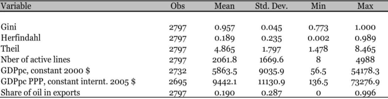
Table 1 shows descriptive statistics for these indices.

Table 1 Descriptive statistics – 156 countries over 1988-2006

Observe that Gini indices are very high. The reason has to do with the level of disaggregation: we use a very disaggregated trade nomenclature. At that level we have a large number of product lines with small trade values, while a relatively limited number of them account for the bulk of all countries’ trade (especially so of course for developing countries but even for industrial ones). As for the average number of “positive” export lines –active lines with non-zero trade values—it is relatively low at 2’062 per country per year, i.e. a little less than half the total, with a minimum of 8 for Kiribati in 1993 and a maximum of 4’988 for

Germany in 1994 and the United States in 1995. This implies that there is room for a substantial “extensive margin” for developing countries, especially the poorest and least diversified ones.

Per-capita GDPs are taken from the World Bank’s World Development Indicators (WDI) and are expressed in 2005 Purchasing Power Parity (PPP) dollars for comparability.

2.2 Parametric evidence

Figure 1 depicts curves representing predicted values of Theil’s index as well as curves representing the predicted number of active export lines.4

The latter, which is concave and increasing at the origin, is easy to distinguish from the former, which is convex and decreasing at the origin.

Figure 1 Predicted Theil’s concentration index & number of active export lines

The “Theil” curve is fitted using quadratic polynomial regressions of the Theil concentration index on per-capita GDP using pooled OLS with White-corrected standard errors. We find a turning point around $30’000 in PPP (2005 constant).5 _{We also estimated “smoother”}

non-parametric regressions (dashed curves). This consists of re-estimating the regression for overlapping samples centered on each observation Smoother regressions impose no functional form and are therefore

4 _{Fitted curves for Herfindahl and Gini indices have similar shapes.}

5 _{We also explore the turning point’s stability across different definitions of GDP}

per capita (i.e., per capita GDP at PPP from the Penn World Tables and per capita GDP in constant US dollars from the WDI). Results, which are similar across definitions, are available upon request.

8

suited to the exploration of highly linear relationships. The non-parametric estimates validate the use of a quadratic form to

approximate the relation between the export concentration and per capita GDP (Figure 1).

One issue is whether the turning point is driven by microstates and island economies which are very heterogeneous in GDP per capita and at the same time very concentrated --say, in bananas or fish products. As microstates are potential outliers, we omit them in the rest of the analysis (i.e., we exclude 15 countries with populations below one million).

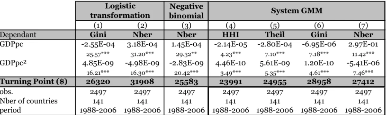
A second issue is that of omitted variables. First, spurious correlation could be introduced by fluctuations in the world price of oil and other commodities, as higher commodity prices would raise both per capita incomes and export concentration for primary-product exporters. The first block of Table 2, which reports pooled estimates with time effects, shows a turning point around 25,000 PPP international (2005 constant) dollars. This turning point is quite similar to the one found by Imbs and Wacziarg for production and by Klinger and Lederman (2006) for exports on a panel of 130 countries over 1992-2003 ($22’500 in constant 2000 dollars).6

Table 2 Pooled, within and between estimates

Second, given the panel structure of our data set, a natural question is the type of estimator --within, between or pooled-- we should use. Imbs and Wacziarg estimation on production data relies on fixed effects (i.e. within). The second and third blocks of Table 2 show our results using the within and between estimators. The turning point stays significant and at a similar level of GDP per capita. Apart from its level, what matters is which countries are on either side of the turning point. Using Theil regressions, the between and pooled estimators return the same list of 21 countries to the right of the turning point. The within estimator adds only two (Israel and New Zealand).7

6 _{The value of our turning point is not directly comparable to that of Imbs and}

Wacziarg, as they used Summers-Heston per-capita incomes in constant 1985 dollars. They note however that their turning point occurs roughly at the level of income reached by Ireland in 1992. Our turning point corresponds roughly to Ireland’s income level in 1996.

7 _{Measurement errors in explanatory variables, if they are correlated with the error}

term, create a downward bias in estimated coefficients that is especially severe with fixed effects (see Griliches and Hausman, 1986). If present, this would push the turning point to the left compared to pooled and between estimates.

9

Table 3 reports a number of robustness checks. First, we consider censoring, as Gini coefficients are bounded left and right, at zero and one respectively --although neither is binding stricto sensu. We thus perform a logistics transformation whose results are reported in the first bloc of Table 3. The turning point is at the usual level of about $26’000. Second, we correct for the potential endogeneity of GDP per capita to export concentration. As we have no valid outside instrument for GDP per capita for our large panel, we carry out a system-GMM estimation. Results, presented in the table’s last block --columns (4) to (7), show a turning point varying between $24’000 (Herfindahl) and $29’000 (Gini), with the same countries to the right of the turning point.8

Table 3 Robustness

Thus, by and large both the existence of a turning point in export concentration and its location around a GDP per capita of about $22’000-27’000 at PPP in constant 2005 international dollars --a very late point in the development process-- are fairly robust.

A glance at the columns entitled “Nber” in Tables 2-3 shows that there is a clear hump-shaped relation between the number of active export lines and GDP per capita. The turning point for the number of active export lines is always roughly at the same level of GDP per capita as that of the concentration indices (see also figure 1). As the number of lines is a count variable, we also run a negative binomial estimation. Results, reported in column (3) of Table 3 are consistent with previous findings. The rising part of the curve corresponds to the introduction of new products as countries develop (see more evidence below). Its decreasing part illustrates one of the striking findings of this paper --namely, that high income countries tend to “close down” export lines faster than they open up new ones, resulting in re-concentration at the extensive margin. We will return to this point later on.

Thus our analysis, regressing concentration indices and the number of active lines on GDP per capita, shows a hump-shaped relationship between economic development and export diversification. Our next task is to understand what is behind the hump.

8 _{A crucial issue with system GMM (Blundell and Bond, 1998) is the number of}

instruments to use. This number should not exceed the number of individuals in the panel (see Roodman, 2006). We make the standard choice of using two lags for the instruments of the differenced equation and one lag for the instruments of the level equation. Following Arellano and Bond (1991) we use the Sargan/Hansen test of overidentifying restrictions and a direct test for the absence of second-order serial correlation; both fail to reject the null of no serial correlation.

10

3. Stages of diversification: “extensive” vs.

“intensive” margins

That export diversification would proceed in parallel with economic development is something to be expected. Pretty much like human beings colonized new land to alleviate competitive pressure on existing pastures, entrepreneurs can be expected to look for “new pastures” and open up production and export lines at the extensive margin. As capital accumulates, this becomes easier. But the later re-concentration, although consistent with Imbs and Wacziarg’s findings for production and employment, is somewhat of a puzzle. In order to better understand what is behind the hump in the curve, we now turn to a systematic analysis of the intensive and extensive margins using the

decomposability property of Theil’s index.

The non-monotone pattern of diversification revealed in Section 2 (decreasing concentration up to $25’000 and increasing concentration thereafter) could be explained by change at the extensive margin, the intensive margin, or both. Diversification at the extensive margin occurs when the number of active lines rises. Diversification at the intensive margin occurs when the distribution of trade values across existing export lines becomes more even. That is, diversification at the intensive margin during a period t₀ to t₁means convergence in export shares among goods that were exported at t₀. The evolution in the number of active lines identified in Section 2 is suggestive of action at the extensive margin. In order to shed more light on the issue, we turn to a

decomposition of Theil’s index which can be usefully mapped into the intensive and extensive margins thus defined.

3.1 Mapping the Theil decomposition with the

extensive and intensive margins

In this section, we combine the classic decomposition of Theil’s index into between- and within-groups components with a partition of export lines into active and inactive ones. The result is a perfect mapping of changes in the between-groups component of Theil’s index into changes in the extensive margin of exports, and of changes in its within-groups components into changes in the intensive margin of exports.

Theil’s index has the property that it can be calculated for groups of individuals (export lines) and decomposed additively into within-groups and groups components (that is, the within- and between-groups components add up to the overall index). Specifically, let n be the total number of potential export lines (the 4’991 lines of the HS6

11

that total number of potential exports (of a given country in a given year) into J+1 groups denoted Gj, j = 0,…,J. Let nj be the number of export lines in group j and

µ

_j their average dollar value. Let also T_j stand for Theil’s index for group j, calculated using (1) on the njlines making up group j. Finally, let x_k be the dollar value of export line k, irrespective of which group it belongs to. The between-groups

component of Theil’s index is defined as

TB = nj n

µ

_j

µ

ln

µ

_j

µ

      j= 0 J

∑

(2)

and its within-groups component is defined as:

TW = nj n j= 0 J

∑

µ

j

µ

Tj = nj n j= 0 J

∑

µ

j

µ

1 nj xk

µ

j k∈G_j

∑

ln xk

µ

j               (3)

It is easily verified that TW

+ TB = T .

Suppose that, for a given country and year, we partition the 4’991 lines making up the HS6 nomenclature into two groups: G1 is made of active

export lines for that country and year, and G0 is made of inactive export

lines. We want to use this partition to construct group Theil sub-indices, one for each group j = 0,1, and the within and between components of the Theil. The between-groups sub-index is not defined since xk = 0 for

all k in G0, so thatµ₀ = 0 and consequently the logarithm in expression

(2) is not defined for j = 0. However, applying L’Hôpital’s rule gives

lim_µ 0→0

µ

₀

µ

ln

µ

₀

µ

             = 0; (4)

so, given our partition

lim_µ 0→0 TB = n1 n µ₁ µ ln µ₁ µ       . (5)

12 As

µ

= x_k / n k=1 n

∑

, µ₁= x_k / n₁ k∈G₁

∑

, and lim_µ 0→0 xk = xk k=1 n

∑

k∈G₁

∑

(since lines

outside G1 must all tend to zero for their mean to also tend to zero) it

follows that n₁µ₁→ nµ, so lim_µ 0→0 TB = ln

µ

1

µ

      = ln n n₁       . (6)

Letting ∆ denote a period-to-period change and observing that n is time-invariant, we have finally that

limµ0→0

∆TB = −∆ ln n₁. (7)

That is, given our partition, changes in the between-groups component of Theil’s index measure changes at the extensive margin (proportional changes in the number of active lines).

As for the “within-groups” component, it is a weighted average of terms combining group-specific means (

µ

_j /

µ

) and group-specific Theil indices T_j (the terms in square brackets), the weights being nj/n. In our

case, TW

reduces to

T1, the group Theil index for active lines. To see this, write (3) in full as

TW = n0 n

µ

0

µ

1 n0 xk

µ

0 k∈G₀

∑

ln xk

µ

0           + n1 n

µ

1

µ

1 n1 xk

µ

1 k∈G₁

∑

ln xk

µ

1          . (8)

In group G0, suppose that all lines have the same arbitrary, strictly

positive value x0, so

µ

0 = x0. Then the first term in (8) is well-defined and boils down to

n₀ n

µ

₀

µ

ln 1

( )

= 0 .

Moreover, this remains true as x0 is made arbitrarily close to zero. Thus,

limx₀→ 0T W = n1 n

µ

1

µ

1 n₁ x_k

µ

1 k∈G1

∑

ln xk

µ

1           . (9)

Now, as x0 tends to zero, we noted already that n₁

µ

₁→ n

µ

; it follows

13 limx₀→ 0T W = 1 n1 xk

µ

1 k∈G₁

∑

ln xk

µ

1     = T1. (10)

Thus, given our partition, changes in the within-groups Theil index ( ∆TW

) measure changes at the intensive margin ( ∆T1, i.e. changes in concentration among active lines only).

In sum, the decomposition of Theil’s index with our partition of export lines into active and inactive ones allows distinguishing changes in overall concentration into extensive- and intensive-margin changes. The evolution of the between component of the Theil corresponds to changes at the extensive margin whereas the evolution of the within component of the Theil reflects changes at the intensive margin.

We now put this decomposition to work. Figure 3 depicts the

contribution of the between and within components to the overall Theil. We observe that, in levels, the “within” component dominates the index; but in terms of evolution, most of the action is in the between

component. 9

Figure 2 “Within” and “between” components of Theil’s index

Until about PPP$22’000, the between component shrinks faster than the within, so diversification occurs mostly at the extensive margin. Past that point and until the turnaround (at around PPP$25’000) it is the within component that decreases fastest, so diversification occurs mostly at the intensive margin. That is, individual export values (and shares) converge among active lines.

Beyond the turning point, the index starts rising again and its rise is driven almost exclusively by the between component. That is, re-concentration occurs at the extensive margin, as countries close down active export lines. What are those lines?

Appendix table A.1 shows the sectors and chapters mostly concerned with closure. The majority of chapters listed in Table A.1 are declining industries in high-income countries. Among the 15 chapters which experienced the highest number of closed lines, three belong to the Textiles sector, a fourth concerns Raw Hides and Skins and Leather , two belong to the Vegetable Products sector, two other to the Live

9 _{When the slope of the overall Theil is at least twice that of its within component,}

the between component contributes for more than 50% to the overall index’s decrease.

14

Animal and Animal Products, two are from the Mineral Products sector and one concerns Iron and Steel. Textiles (Chapter 53) and Leather (Chapter 41) are among the most active “closers” (8.6% of the chapter’s active lines for the former, 9.4% for the latter). The case of Chemicals (Chapter 29 and 28), is worth investigating. Although the Chemicals sector does not necessarily come across as a declining sector for most developed countries (Figure 4b confirms that high-income countries specialize in chemicals), chapters 29 and 28 rank high in their number of closed lines. The simultaneous occurrence of rising specialization and line closures in the chemical sector is however consistent with Schott’s (2004) finding that specialization occurs within sectors, as high-tech exports replace low-tech ones when countries grow. The closure of export lines in the leather sector, by contrast, suggests between-product specialization, as leather or cotton works are labor-intensive activities in which countries lose comparative advantage when they grow. We will explore more intensively this last point section 4.

3.2 What are the “new export products” that

generate trade diversification?

Although the most intriguing feature of the U-shape pattern is the exports’ re-concentration of the richest countries, patterns of

diversification at lower income levels are also of interest. As most of the diversification occurs at the extensive margin, one may indeed wonder what the characteristics of those “New export products” (i.e. new lines at the HS6 level) are.

The number of new export products should be interpreted somewhat cautiously, as new export products are not necessarily true

entrepreneurial “discoveries”. In most cases, they correspond to the opening of new export lines that are already active in other countries. This is particularly true for developing countries copying existing products invented elsewhere and exporting those products as new export lines. In contrast, genuine innovations are incorporated within the HS6 classification in the course of periodic revisions and may not show up as new exports lines.10 _{Our new export products thus}

correspond to what Klinger and Lederman (2006) called “inside-the-frontier innovations”. The focus of our paper is not innovation, but export diversification within an existing (although arbitrarily limited)

10 _{At the HS6 level, reclassifications are limited, but we follow Besedes and Prusa}

(2006a) in treating them as censored; that is, a spell of, say, five years ending with a reclassification is treated as a spell of at least five years, like one at the end of the sample.

15

product nomenclature. Exporting a product for the first time (i.e., opening a new export line) even if it were already produced or exported to other destinations, is an entrepreneurial risk which is worth

investigating.

There is no conventional definition of new export products. In order to stay as close as possible to the definition of active lines and in the tradition of Besedes and Prusa (2006b), we first define “new export products” for a year and country as those lines that were not active in the country’s export trade in the preceding year but were exported in the following year (one year cut-off). This definition, based on a moving 3-year window, reduces the sample period to 1989-2005, one 3-year being taken out at both ends. As alternatives, we use (i) Klinger and

Lederman’s (2006) definition (discussed below); (ii) lines that were inactive in the country’s export trade in the preceding two years but were exported in the following two years (two years cut-off). This latter definition strikes a balance between the very conservative definition used by Klinger and Lederman (2006) and the very liberal one used by Besedes and Prusa (2006b).

Klinger and Lederman (2006) define “discoveries” as products not exported in the early part of their sample (1994-1996) but with over $10’000 of exports in the latter part (2002-2003). What is the

difference between this definition and definitions that account for years of inactivity and activity around the first appearance of a product (one year or two years cut-off)? Conceptually, these notions of new export products are essentially the same, being based on the idea that imperfectly-informed entrepreneurs search for profitable export opportunities. Uncertainty can be about production costs, as in Hausmann and Rodrik (2003), or about foreign demand, as in Vettas (2000); but the point is that starting to export a product is an

entrepreneurial gamble that may fail. Whereas Klinger and Lederman’s definition singles out successful export-line development (new lines that reach a threshold value), the other definitions include small-volume, short-spell lines in order to pick up the trial-and-error process at the extensive margin. The shorter the spells, the more discoveries or new products there should be, as new entrepreneurs try again a few months or years later. Detailed evidence on the length of export spells was recently analyzed by Besedes and Prusa (2006a), who found that over half of all trade relationships were observed for a single year and 80% lasted less than five years. Our more aggregated HS6 data is likely to smooth some of those entries and exits, but Besedes and Prusa showed the high churning rate to be robust to aggregation.

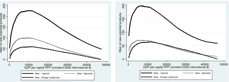
Figure 3 shows the predicted number of new export products (per country-year, with several alternative definitions of new export products) against GDP per capita using the non-parametric

(“smoother”) estimator. In all cases, the turning point comes very early --in the PPP$ 5’000 to 10’000 range. The rapid decrease in “export

16

entrepreneurship” apparent in the figure could conceivably be due to equally rapid convergence toward the absolute barrier to diversification (the five thousand lines of the HS system); but it is not, as few countries approach this barrier and certainly not those at GDP per capita levels around $5’000 to $10’000.11

Figure 3 Predicted New Exports: non-parametric estimates

The relationship between income and new export products is robust to the choice of definition of “new products”. The lower number of Klinger and Lederman’s “new export products” in Figure 3a could be expected from the more conservative aspect of their definition. It could also result from the shorter time length on which new products are measured. As 10 years are required to compute a new product à la Klinger and Lederman, we measured these new products on the 1997-2006 period, against 1989-2005 for the Besedes and Prusa definition (one year cut-off) and 1990-2004 for the two years cut-off. Figure 3b depicts the non-parametric estimates of the predicted number of new export products against GDP per capita for the 1997-2005 period which is common to all definitions. Once corrected for the number of years available, new export products à la Klinger and Lederman are similar to new export products defined by the two years cut-off. The one year cut-off

unsurprisingly counts more new products as it includes several of these new exports with extremely short spells, which can be assimilated to trial-and-error export products.

We finally ask whether new export products are any different from other traditional exports. Table 4 gives a characterization of export goods using Rauch’s index of product differentiation. Rauch (1999) distinguished between products traded on organized exchanges, products with reference prices, and differentiated ones. Table 4 shows the proportion of each of Rauch’s categories in traditional and new export lines as measured according to Besedes and Prusa (2006b) definition. Using other definitions for new export products provides similar shares.

Table 4 Characterization of products by degree of differentiation

We find a lower share (in terms of export value) of homogenous-product exports among new than among traditional ones (15.0% vs. 39.1% using Rauch’s “conservative” classification and 22.6% vs. 41.3% according to his “liberal” classification). The reverse is true for “reference-priced” and

17

differentiated goods, suggesting that the bulk of diversification is made on these types of products. This feature is emphasized by the proportion of each Rauch’s categories in term of the number of new lines.

Differentiated goods account for 61.2% to 64.4% of new export lines in average over the 1989-2005 period.

Finally as Besedes and Prusa (2006b) and Rauch and Watson (2003), we observe that initial trade in homogenous products requires higher values than initial trade in differentiated products. The proportion of homogeneous goods in the total number of new export lines is smaller than its proportion in the total value of these new exports (7.6% vs. 15.0% using Rauch’s “conservative” classification and 12.0% vs. 22.6% according to his “liberal” classification). The contrary is true for differentiated products (64.4% vs. 52.5% using Rauch’s “conservative” classification and 61.2% vs. 49.2% according to his “liberal”

classification).

Thus, new export products are essentially low-value differentiated goods traded by low-income countries. These findings are consistent with the existing literature. Interestingly, they are independent of the definition chosen.

4. Stages of diversification: Alternative

explanations

Our decomposition of the Theil index highlights the importance of distinguishing the extensive from the intensive margins in the evolution of export diversification. It also suggested a conjecture of slow

adjustment across diversification cones (Section 4.3). We must however consider alternative explanations which could artificially create or reinforce a hump-shaped pattern. The diversification curve may e.g. result from spurious statistical effects. Alternative explanations include (i) the potential role of primary-resource exports as large exporters of mineral products (those for which mineral products represent over 50% of exports) are either low/middle income countries or very high-income ones in our database (section 4.1); (ii) the structure of the HS6

COMTRADE classification, as textiles and clothing, essentially exported by low to middle-income countries, have a large number of lines per dollar of export (section 4.2). We show in the next section that the hump-shaped relationship is robust to controls for these alternative explanations, and then explore characteristics of closed lines that may help understand what drives the hump shape.

18

4.1 Primary products

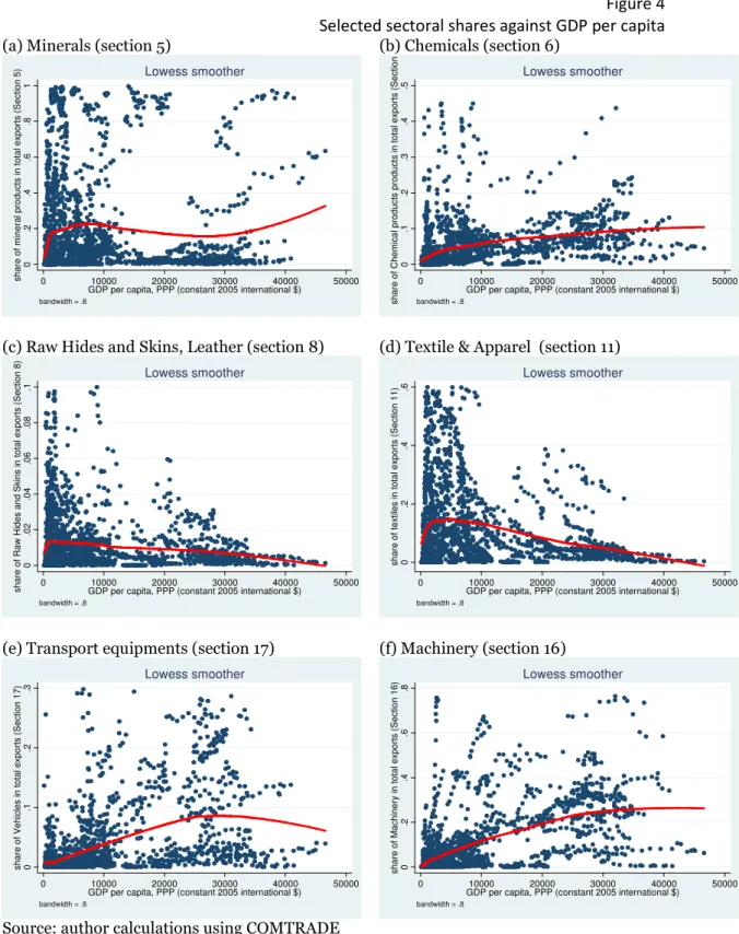
We consider here the prevalence of primary resources in exports as an explanation for the U-shaped pattern of export concentration evidenced in section 2. Where do we find large primary-resource exporters along the income axis? Figures 4 shows selected sectoral shares against GDP per capita.

Figures 4a-4f Selected sectoral shares against GDP per capita

Figure 4a) for minerals (HS section 5) shows a fairly distinct pattern whereby large exporters of mineral products (those for which mineral products represent over 50% of exports) are either low/middle income countries or very high-income ones. This pattern, which is confirmed by the non-parametric regression curve, is of course likely to contribute to the U-shaped pattern of export concentration.

As the “large primary-product exporter” status is a largely

time-invariant country characteristic, the country fixed-effects estimator used in section 2 already suggests that the U-shaped pattern of export

concentration is not a spurious one due to primary product exports. However, given the importance of primary product exports in the debate linking export concentration and development, we choose to go beyond the “country fixed effects” approach in two ways.

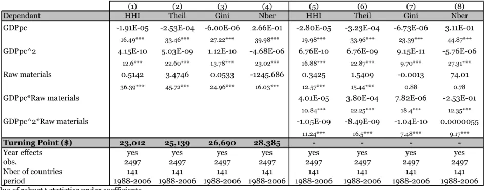
First, we exploit the time variation in the share of primary products in exports over the 1988-2006 period by including this variable (in an additive way) in our usual quadratic. We thus introduce in the model the share of HS chapters 26 (ores, slag and ashes) and 27 (mineral fuels, mineral oils and products of their distillation).12 _{Results are shown in}

Table 5.

Table 5 Estimates with raw-material export shares

Unsurprisingly, the share of raw materials comes out as a positive and significant contributor to export concentration (this is to be expected, as a large share of one narrow class of products is likely to be associated with high concentration) and as a negative one to the number of active lines (first block of Table 5). But the striking result is that coefficients on GDP per capita and its square are not affected by much; nor is the turning point.

19

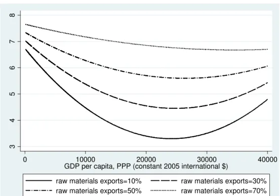
Second, we want to know if the share of raw materials only changes the level of export concentration or if it also has an impact on the

magnitude of the U-shape and on the level of the turning point . We thus interact the share of raw materials in exports with GDP per capita (second block of Table 5). Figure 5 plots predicted Theil indices against GDP per capita for various levels of raw-material export shares.

Figure 5 Predicted Theil indices against GDP per capita and the share of raw materials in export

Except for very high values of the share of raw materials (over 70%), the U-shaped relationship is maintained with an almost unchanged turning point.

4.2 The Harmonized System’s classification

The harmonized system’s classification used by COMTRADE could also potentially explain the hump-shaped relationship between economic development and export diversification. This classification is derived from nomenclatures originally designed for tariff-collection purposes rather than to generate meaningful economics. Consequently, some sections have a large number of economically irrelevant categories (e.g. the textile-clothing sector −section 11), whereas in other sections (e.g. machinery −section 16) economically important categories are lumped together in a few lines. Now, assume that products in section 11 are essentially exported by middle-income countries whereas products in section 16 are essentially exported by high income countries

(assumptions confirmed by Figures 4d and 4f respectively). Then, the observed diversification/re-concentration pattern could be an illusion caused by the structure of the HS6 classification.

Figure 6a, which plots, for each section of the HS6 classification, total export value versus number of lines provides evidence of this feature. Section 6, 11, 15 and 16 have a much higher number of lines than others sectors of the HS6 classification. Section 16 however differs from Section 6, 11 and 15 as it is well above the 45° line, reflecting a

disproportionate high value per export line, whereas sections 6, 11 or 15 include a large number of small lines.

Figure 6 Trade value vs. number of lines, by section

In order to control for the conjecture that the U-shape pattern of diversification may be a consequence of the structure of the HS6 classification, we went back to our raw database and re-aggregated the lines in sections 6, 11 and 15 from HS6 (sub-Heading) to HS4 (Heading) level (because of its specificity, we treated Section 16 separately as

20

explained below). The number of lines in these sectors thus shrinks drastically, reducing the average value per line to a level comparable to that of other sections, as reported in Figure 6b.

Our new classification (HS4 for sections 15, 6 or 11 and HS6 otherwise) includes 3,336 products lines instead of 4,991 for the benchmark classification. Results obtained with Theil indices calculated on the modified database are not significantly different from the ones obtained above: The turning point is consistent with previous findings under pooled or within estimation.13

Figure 6 reveals that section 16 has both a large number of lines and a disproportionate high value per export line (the section represents around 25% of the total value of exports). The high value per export lines suggests that the number of existing lines is not extended enough to represent production in this section in a similar way as other sections of the HS6 classification. Mammoth lines may indeed include much more products than lines in other sections. This could artificially lead to the high concentration of high income countries.

We thus need to control for the particular design of section 16. As we can not further disaggregate section 16, we dropped this sector from the database. Our final classification thus includes 2575 product lines. Results (not reported here but available upon request) are similar to the one obtain with the benchmark classification: The turning point is robust to the aggregation of Section 6, 11 or 15 and the elimination of Section 16 in the pooled as well as in the within estimation.

The hump-shaped relationship between economic development and export diversification is thus not a consequence of spurious

“composition” effects.14

4.3 Traveling across diversification cones

As Schott (2003, 2004) and Xiang (2007) discussed, countries travel across diversification cones when they accumulate capital. As they do, “old-cone” lines should become inactive while “new-cone” ones should become active. Suppose that “old-cone” lines are slow to die because of incumbency advantages, established ties with customers, or any kind of support they may get. During the transition phase, then, new-cone lines

13 _{Results available upon request.}

14 _{We also ran our baseline concentration regression with the share of service}

exports in GDP on the right-hand side. Results (available upon request) were unchanged: the turning point was nearly the same. We thank Carsten Fink for giving us the service data.

21

become active while old-cone ones don’t want to die. As a result, exports diversify and the total number of active lines rises. As time passes, however, comparative advantage catches up on old lines and they slowly die, reducing diversification. Viewed this way, high diversification at middle-income levels is essentially a transitory phenomenon between two steady states in terms of industrial specialization.

Besedes and Prusa’s finding that the hazard rate decreases rapidly in the first years of an export spell is indeed suggestive of a dual regime with high infant mortality, consistent with Hausmann and Rodrik’s view of an entrepreneurial trial-and-error process, and persistence among “old” spells, consistent with the conjecture above. It is also consistent with Schott’s (2003) finding that “[…] estimated development paths deviate substantially from the theoretical archetypes of Figures 4 [i.e. a

systematic pattern of births for “new-cone” industries and deaths for “old-cone” ones]. Many sectors, including Apparel and Footwear, exhibit positive value-added per worker in more than two cones” (pp. 693-6). Apparel and footwear could indeed be slow-dying industries in many countries, not only on the import-competing side but also on the export side (the EU for instance is still today a major exporter of textile and apparel products). If that were the case, the high diversification characterizing the middle part of the economic development process would not be a desirable outcome per se but simply an

out-of-equilibrium one characterizing the transition from one steady state to another, each characterized by specialization according to comparative advantage.

A comparison of Figures 4d and Figure 4f, which show respectively the shares of textile and apparel products (section 11) and machinery (section 16) in exports as a function of GDP per capita, partly bears out this story, as the former follows a decreasing and only mildly convex trajectory (see the smoother fitted curves) while the latter follows a rising and concave one. The combination of the two generates a decrease in export concentration up to the $10’000 threshold, after which there isn’t much action any more as both textiles and machinery stabilize at low (5%) and high (30%) shares respectively.

Suppose that when a country re-concentrates, export lines that it closes are “old-cone” lines that were still in that country’s export portfolio essentially by inertia. In that case, lines closed by a country to the right of the diversification turning point would lie further from its

comparative advantage than lines closed, in the process of normal churning, by countries to the left of the turning point.

This is a conjecture we can verify, albeit indirectly. To do this, we use a database compiled by Cadot, Shihotori and Tumurchudur (2008). The databases contains national factor endowments (capital per worker and educational achievement) as well as “revealed” factor intensities

22

endowments of countries exporting each good. The construction of these revealed factor intensities follows the logic of Hausmann, Hwang and Rodrik’s (2007) PRODY. That is, the revealed capital intensity of product k is

ˆ_{k ik i}

i

κ

=

∑

ω κ

(11)

where κ_iis country i’s capital/labor endowment calculated à la Easterly-Levine (2001) and ω_ikis its (Balassa) index of revealed comparative advantage in good k. Human-capital intensities (i.e., h_ifor country i) are from Barro and Lee’s national educational achievements database, and the revealed human-capital intensity of product k is calculated in a way similar to (11). We compare the revealed factor intensity of closed line k, computed this way, with the endowment of the country closing it, using a Euclidian distance formula

(

)

(

)

1/2 2 ₂ ˆ _ˆ e ik i k i k d =_ h −h + κ −κ _   . (12)

If our conjecture were true, d_ike should be larger for lines closed by countries to the right of the turning point (declining industries) than for lines closed by countries to the left of it (normal churning). Panel a) of Figure 7 shows just that pattern. The density ofd_ike for lines closed by countries to the left of the diversification turning point (solid blue line) peaks near the vertical axis, suggesting small distances between their factor intensities and the endowments of countries closing them (“accidental” closures).15 _{By contrast, the density of d}

ik e

for lines closed by countries to the right of the turning point (broken red line) peaks far from the vertical axis, suggesting large distances (products far from the closing country’s current diversification cone). To make the argument plain, the average intensity of lines closed by countries to the right of the turning point is between the factor endowments of Chile and Malaysia, whose income is about half the turning point.

15 _{In order to limit the number of one year trial-and-error cases in our estimation,}

we define closed lines, in a similar way as “new export lines”, as lines that had been open for 2 years and remained subsequently closed for 2 years. The kernel

estimation is thus performed on lines closed between 1990 and 2003 (endowment-intensity distances are not available in Cadot et al. (2008) database for 2004). Note that we also run the exercise defining closed lines as lines that had been open for 1 year and remained subsequently closed for 1 year. Although there are around five times more closed lines with this definition, we observe the same patterns that the ones described in this section.

23

Panel b) of Figure 7 provides a counterfactual. Densities estimated in a similar way for new export lines peak near zero, suggesting that the factor intensity of new export lines coincides roughly with the

endowment of the countries introducing them. Moreover, there is no clear difference between the lines introduced by countries to the right of the turning point and those introduced by countries to the left.

Figure 7 Kernel density of endowment-intensity distances for closed lines

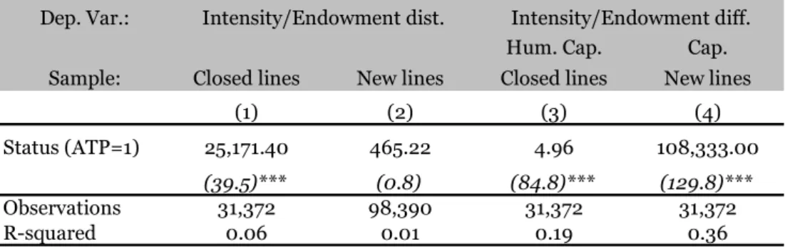
In order to go beyond descriptive statistics, we regressed endowment-intensity distances (d_ike) on the status of countries (i.e., a dummy variable equal to one for countries to the right of the turning point and zero otherwise) first on the sub-sample of closed lines, and then on the sub-sample of new lines for the counterfactual. Table 6 presents the results (see columns (1) and (2) respectively) and confirms the findings of Figures 7. The coefficient on the status dummy is positive and

significant for closed lines, but insignificant for new lines.

Table 6 Regression results, endowment/intensity distances on closed line status

Columns (3) and (4) show that the factor intensities of lines closed to the right of the turning point are not just far from the endowments of the countries closing them, but also less intensive in human capital and capital. That is, in column (3) the dependent variable is d_ikh = h_i − h_k , and in column (4) it is d_ikκ =

κ

_i−

κ

_k. The status dummy is again positive and highly significant.

The evidence brought together in this section is only suggestive of a pattern whereby the closure of export lines in declining industries is delayed, but it certainly goes in that direction. It also confirms the prima-facie evidence in Annex Table A.1, where declining industries figure prominently among closed lines.

5. Concluding remarks

The results presented so far suggest two observations. First, there seems to be, across countries and time, a robust hump-shaped relationship between export diversification and the level of income (the mirror image of our U-shaped concentration indices). This non-monotonicity holds both between and within countries. The re-concentration of exports above a threshold around PPP$25’000 is especially striking.

Diversification occurs mostly at the extensive margin, especially early on in the development process, as new export items multiply and are

24

marketed at increasingly large initial scales. This relationship does not appear to be spurious or driven only by variations in the share of primary products. From a policy perspective, it thus appears as a key element of the economic development process and is, if not necessarily an objective per se, at least an important policy indicator. From an econometric perspective, our findings justify treating export

diversification as endogenous in growth regressions, as de Ferranti et al. (2002) do.

The second observation is that diversification at middle to high levels of income may simply reflect a slow adjustment process between two equilibria, with new export sectors being faster to appear than old ones are to die. We find evidence that countries to the right of the turning point close lines that are typically, in terms of factor intensities, far from their endowments—so to speak, outliers in their export portfolios. The hump-shaped relationship between diversification and development may be explained by this slow adjustment as countries travel across diversification cones.

25

References

Auty, R., (1990), Resource-based industrialization: Sowing the oil in eight developing countries; Oxford University Press.

Arellano, M., and S. Bond (1991), “Some tests of specification for panel data: Monte Carlo evidence and an application to employment

equations”, Review of Economic Studies 58, 277–97.

Barro, R. J. and J-W Lee (2000), “International Data on Educational Attainment: Updates and Implications”, CID Working Paper #42. Besedes, T., and T. Prusa (2006a), “Surviving the U.S. Import Market: The Role of Product Differentiation”, Journal of International

Economics, 70, 339-358.

− and − (2006b), “Ins, Outs, and the Duration of Trade”, Canadian Journal of Economics 39, 266-95.

Blundell, R., and S. Bond (1998), “Initial conditions and moment

restrictions in dynamic panel data models”, Journal of Econometrics 87, 11–143.

Brenton, P., and R. Newfarmer (2007), “Watching more than the Discovery channel : export cycles and diversification in development”; Policy Research Working Paper #4302, The World Bank.

Brunnschweiler, C. (2008), “Cursing the blessings? Natural resource abundance, institutions, and economic growth”, World Development 36, 399-419.

--, and E. Bulte (2008), “Linking Natural Resources to Slow Growth and More Conflict”, Science 320 (5876), 616-617.

Cadot, O., Shirotori M. and B. Tumurchudur (2008), “Revealed Factor Intensities at the Product Level”, mimeo, UNCTAD.

Dutt, P., Mihov I. and T. Van Zandt (2008), “Trade Diversification and Economic Development”, mimeo, INSEAD.

Easterly, W. and R. Levine (2001), "It's not Factor Accumulation: Stylized Facts and Growth Models", World Bank Economic Review 15, 177-219.

Evenett, S. and A. Venables (2002): “Export Growth in Developing Countries: Market Entry and Bilateral Trade Flows”, mimeo.

de Ferranti, D., Perry, G., Lederman, D. and W. Maloney (2002), From Natural Resources to the Knowledge Economy; The World Bank.

26

Gelb, A. (1988), Windfall gains: Blessing or curse?, Oxford University Press.

Griliches, Z., and J. A. Hausman (1986) „Errors in variables in panel data”, Journal of Econometrics 31, 93-118.

Hausmann, R. and D. Rodrik (2003), “Economic Development as Self-Discovery”, Journal of Development Economics 72, 603-633.

−, Hwang J. and D. Rodrik (2007), “What You Export Matters”, Journal of Economic Growth 12, 1-25.

− and B. Klinger (2006), “Structural Transformation and Patterns of Comparative Advantage in the Product Space”, mimeo, Harvard University.

Hummels, D. and P. Klenow (2005), “The Variety and Quality of a Nation’s Exports”, American Economic Review 95, 704-723.

Imbs, J. and R. Wacziarg (2003), “Stages of Diversification”, American Economic Review 1993, 63-86.

Kehoe, T. J. and K. J. Ruhl (2006), “How Important is the New Goods Margin in International Trade?”, 2006 Meeting Papers 733, Society for Economic Dynamics.

− and D. Lederman (2004), “Discovery and Development: An Empirical Exploration of ‘New’ Products”, mimeo.

− and − (2006), “Diversification, Innovation, and Imitation inside the Global Technology Frontier”, World Bank Policy Research Working Paper #3872, The World Bank.

Neary, R. and S. van Wijnbergen, eds. (1986), Natural resources and the macroeconomy; MIT press.

Prebisch, R. (1950), “The Economic Development of Latin America and its Principal Problems”, reprinted in Economic Bulletin for Latin America 7, 1962, pp. 11-22.

Rauch, J. (1999), “Networks versus Markets in International Trade”, Journal of International Economics 48, 7-35.

Rauch, J. and J. Watson (2003), “Starting Small in an Unfamiliar Environment”, International Journal of Industrial Organization 21, 1021-1042.

Roodman, D. (2006), “How to Do xtabond2: An Introduction to

‘Difference’ and ‘System’ GMM in Stata”; Center for Global Development Working Paper #103.

27

Sachs, J. and A. Warner (1999), "The Big Rush, Natural Resource Booms And Growth", Journal of Development Economics 59, 43-76.

Schott, P. (2003), “One Size Fits All? Heckscher-Ohlin Specialization in Global Production”, American Economic Review 93, 686-708.

− (2004), “Across-product versus Within-product Specialization in International Trade”, Quarterly Journal of Economics 119, 647-678. Singer, H. (1950), “US Foreign Investment in Underdeveloped Areas: The Distribution of Gains Between Investing and Borrowing Countries”, American Economic Review 40, 473-485.

Theil, H. (1972), Statistical Decomposition Analysis; North Holland. Vettas, N. (2000), “Investment Dynamics in Markets with Endogenous Demand”, Journal of Industrial Economics 48, 189-203.

Xiang, C. (2007), “Diversification cones, trade costs and factor market linkages”, Journal of International Economics 71, 448-466.

28

Tables and figures

Tables

Table 1 Descriptive statistics – 156 countries over 1988-2006

Variable Obs Mean Std. Dev. Min Max

Gini 2797 0.957 0.045 0.773 1.000

Herfindahl 2797 0.189 0.235 0.002 0.989

Theil 2797 4.865 1.797 1.478 8.465

Nber of active lines 2797 2061.8 1669.6 8 4988

GDPpc, constant 2000 $ 2732 5863.5 9035.9 56.5 54178.3

GDPpc PPP, constant internt. 2005 $ 2695 9442.1 11130.9 136.5 73276.9

Share of oil in exports 2797 0.190 0.287 0 0.996

29

Dependent HHI Theil Gini Nber HHI Theil Gini Nber HHI Theil Gini Nber GDPpc -1.89E-05 -0.0002516 -5.98E-06 2.65E-01 -6.50E-06 -0.0000779 -2.63E-06 3.90E-01 -1.89E-05 -0.0002573 -5.84E-06 2.68E-01

12.48*** 23.40*** 21.34*** 36.53*** 2.22*** 4.91*** 9.46*** 23.96*** 2.57** 4.85*** 4,52*** 7.68*** GDPpc² 4.09E-10 4.99E-09 1.12E-10 -4.67E-06 1.38E-10 1.83E-09 5.87E-11 -6.98E-06 4.21E-10 5.20E-09 9.95E-11 -4.79E-06

9.49*** 15.40*** 10.27*** 21.00*** 2.52*** 6.18*** 11.27*** 18.67*** 1.90* 3.11*** 2.00** 4.26*** Turning Point ($)23,105 25,210 26,744 28,396 23,551 21,284 22,402 27,928 22,447 24,740 29,347 28,012 R2 0.12 0.37 0.50 0.64 0.10 0.32 0.43 0.58 0.10 0.36 0.51 0.63 obs. 2497 2497 2497 2497 2497 2497 2497 2497 141 141 141 141 Nber of countries 141 141 141 141 141 141 141 141 141 141 141 141 period 1988-2006 1988-2006 1988-2006 1988-2006 1988-2006 1988-2006 1988-2006 1988-2006 1988-2006 1988-2006 1988-2006 1988-2006

Australia Australia Australia Australia Australia Australia Australia Australia Australia Australia Australia Australia Austria Austria Austria Austria Austria Austria Austria Austria Austria Austria Austria Austria Belgium Belgium Belgium Belgium Belgium Belgium Belgium Belgium Belgium Belgium Belgium Belgium Canada Canada Canada Canada Canada Canada Canada Canada Canada Canada Canada Canada Denmark Denmark Denmark Denmark Denmark Denmark Denmark Denmark Denmark Denmark Denmark Denmark Finland Finland Finland Finland Finland Finland Finland Finland Finland Finland Finland Finland France France France France France France France France France France France Greece Greece Greece Greece Greece Greece Greece Greece Greece Greece

Germany Germany Germany Germany Germany Germany Germany Germany Germany Germany Germany Germany Hong Kong Hong Kong Hong Kong Hong Kong Hong Kong Hong Kong Hong Kong Hong Kong Hong Kong Hong Kong Hong Kong Hong Kong Ireland Ireland Ireland Ireland Ireland Ireland Ireland Ireland Ireland Ireland Ireland Ireland

Israel Israel Israel Israel

Italy Italy Italy Italy Italy Italy Italy Italy Italy Japan Japan Japan Japan Japan Japan Japan Japan Japan Japan Japan Netherlands Netherlands Netherlands Netherlands Netherlands Netherlands Netherlands Netherlands Netherlands Netherlands Netherlands Netherlands New Zealand New Zealand New Zealand New Zealand

Norway Norway Norway Norway Norway Norway Norway Norway Norway Norway Norway Norway Singapore Singapore Singapore Singapore Singapore Singapore Singapore Singapore Singapore Singapore Singapore Singapore Spain Spain Spain Spain Spain Spain Spain Spain

Sweden Sweden Sweden Sweden Sweden Sweden Sweden Sweden Sweden Sweden Sweden Sweden Switzerland Switzerland Switzerland Switzerland Switzerland Switzerland Switzerland Switzerland Switzerland Switzerland Switzerland Switzerland United King. United King. United King. United King. United King. United King. United King. United King. United King. United King. United King. United King. United States United States United States United States United States United States United States United States United States United States United States United States

Countries on the right of the turning point in 2006

Absolute value of robust t statistics under coefficients. ***, **, * significant at respectively 1%, 5% and 10% level. Note: all sample except microstates, GDP per capita PPP in constant 2005 international $, from WDI

31 Table 3 Robustness Negative binomial (1) (2) (3) (4) (5) (6) (7)

Dependant Gini Nber Nber HHI Theil Gini Nber

GDPpc -2.55E-04 3.18E-04 1.45E-04 -2.14E-05 -2.80E-04 -6.95E-06 2.97E-01

25.57*** 31.20*** 29.32** 4.23*** 7.10*** 7.18*** 11.42***

GDPpc² 4.85E-09 -4.98E-09 -2.83E-09 4.46E-10 5.61E-09 1.20E-10 -5.41E-06

16.21*** 16.30*** 20.42*** 3.49*** 5.35*** 4.61*** 7.46*** Turning Point ($) 26320 31908 25583 23991 24955 28958 27412 obs. 2497 2497 2497 2497 2497 2497 2497 Nber of countries 141 141 141 141 141 141 141 period 1988-2006 1988-2006 1988-2006 1988-2006 1988-2006 1988-2006 1988-2006 Logistic transformation System GMM

Absolute value of robust t statistics under coefficients. ***, **, * significant at respectively 1%, 5% and 10% level.

Note: all sample except microstates, GDP per capita PPP in constant 2005 international $, from WDI

Source: author calculations using COMTRADE

Table 4 Characterization of products by degree of differentiation

New products New products All products World Trade, 1990

(count number) (Rauch) b/

Conservative classification a/ Homogenous 7.6% 15.0% 39.1% 12.6% Reference priced 28.1% 32.5% 27.4% 20.3% Differentiated 64.4% 52.5% 31.9% 67.1% Liberal classification a/ Homogenous 12.0% 22.6% 41.3% 16.0% Reference priced 26.8% 28.2% 19.7% 19.5% Differentiated 61.2% 49.2% 39.1% 64.2%

Notes: in value of total trade unless otherwise indicated.

a/ Because the classification of some products cannot be asserted unambiguously, Rauch’s conservative classification assigns fewer products to the “homogenous” and “reference-priced” categories than his liberal ones.

b/ From Table 2 of Rauch (1999)

32

Table 5 Estimates with raw-material export shares

(1) (2) (3) (4) (5) (6) (7) (8)

Dependant HHI Theil Gini Nber HHI Theil Gini Nber

GDPpc -1.91E-05 -2.53E-04 -6.00E-06 2.66E-01 -2.80E-05 -3.23E-04 -6.73E-06 3.11E-01

16.49*** 33.46*** 27.22*** 39.98*** 19.98*** 33.96*** 23.39*** 44.87***

GDPpc^2 4.15E-10 5.03E-09 1.12E-10 -4.68E-06 6.76E-10 6.76E-09 9.15E-11 -5.76E-06

12.6*** 22.60*** 13.78*** 23.02*** 16.88*** 22.87*** 9.70*** 27.31***

Raw materials 0.5142 3.4746 0.0533 -1245.686 0.3425 1.5409 -0.0013 74.01

36.39*** 45.72*** 24.96*** 16.03*** 12.57*** 15.44*** 0.88 0.78

GDPpc*Raw materials 4.01E-05 3.80E-04 7.82E-06 -2.53E-01

10.84*** 22.25*** 18.4*** 12.35***

GDPpc^2*Raw materials -1.05E-09 -8.49E-09 -1.04E-10 0.0000055

11.24*** 16.5*** 7.48*** 9.17***

Turning Point ($) 23,012 25,139 26,690 28,385 - - -

-Year effects yes yes yes yes yes yes yes yes

obs. 2497 2497 2497 2497 2497 2497 2497 2497

Nber of countries 141 141 141 141 141 141 141 141

period 1988-2006 1988-2006 1988-2006 1988-2006 1988-2006 1988-2006 1988-2006 1988-2006

Absolute value of robust t statistics under coefficients. ***, **, * significant at respectively 1%, 5% and 10% level.

Note: all sample except microstates, GDP per capita PPP in constant 2005 international $, from WDI Source: author calculations using COMTRADE

33

Table 6 Regression results, endowment/intensity distances on closed line status

Dep. Var.:

Hum. Cap. Cap.

Sample: Closed lines New lines Closed lines New lines

(1) (2) (3) (4)

Status (ATP=1) 25,171.40 465.22 4.96 108,333.00

(39.5)*** (0.8) (84.8)*** (129.8)***

Observations 31,372 98,390 31,372 31,372

R-squared 0.06 0.01 0.19 0.36

Intensity/Endowment dist. Intensity/Endowment diff.

Notes: Estimation is by OLS, year dummies are not reported in order to save space. Absolute value of robust t statistics under coefficients. ***, **, * significant at respectively 1%, 5% and 10% level.

The dependent variable in columns (1) and (2) is the Euclidean distance between the factor intensity of closed lines (see text for details on the calculation) and the factor endowment of the country closing it, all for the year in which the closure takes place. In columns (3) and (4), it is the algebraic difference between the factor endowment of the closing country and the factor intensity of the closed line (for human and physical capital respectively). The “status” regressor is a dummy variable equal to one when the line is closed by a country to the right of the turning point in year t. Thus, ignoring the year dummies, column (4) says that

∆K = −22 '909 + 108'333IR (13)

where capital is measured in 2000 PPP dollars and the status dummy I_R is

I_R = 1 if country is to the right of the turning point in t

0 otherwise.     (14) Thus, the negative intercept means that a closed line is on average $22’909 more capital intensive than the endowment of the country closing it when it is left of the turning point, and $108’333-27’909 = $80’424 less intensive to the right of the turning point. By way of comparison, France’s capital endowment (capital per worker at 2000 PPP dollars) was, in 2003, $139’000.