Design and implementation of a fiber optic doppler optical coherence microscopy system for cochlear imaging

Design and Implementation of a Fiber Optic

Doppler Optical Coherence Microscopy System for

Cochlear Imaging

by

Logan P. Williams

S.B., Electrical Science and Engineering, Physics

Massachusetts Institute of Technology (2013)

Submitted to the Department of

Electrical Engineering and Computer Science

in partial fulfillment of the requirements for the degree of

Master of Engineering in Electrical Science and Engineering

at the

Massachusetts Institute of Technology

June 2014

Massachusetts Institute of Technology 2014. All rights reserved.

Author ...

Signature redacted-..

Department of Electrical Engineering and Computer Science

May 15, 2014

Certified by...

Signature redacted

Dennis M. Freeman

Professor of Electrical Engineering

AhA _ThessSprio

Signature redacted

sis

Supervisor

A ccepted by ...

...

Albert R. Meyer

Chairman, Masters of Engineering Thesis Committee

OF TECHNOLOGY

JUL 15

2014

Design and Implementation of a Fiber Optic Doppler Optical

Coherence Microscopy System for Cochlear Imaging

by

Logan P. Williams

Submitted to the Department of Electrical Engineering and Computer Science on May 15, 2014, in partial fulfillment of the

requirements for the degree of

Master of Engineering in Electrical Science and Engineering

Abstract

In this thesis, the design and implementation of a fiber optic Doppler optical coherence microscopy (FO-DOCM) system for cochlear imaging applications is presented. The use of a fiber optic design significantly reduces system size and complexity and the construction of a novel alignment and micropositioning apparatus increases ease of use for the researcher performing the imaging. To enable precise measurements of tissue motion, a time domain DOCM approach is used, utilizing an acousto-optic modulator (AOM) based optical heterodyne system to generate a stationary interference carrier frequency. By referencing this interference signal against the AOM drive signals, measurements of motions with magnitude on the order of 10 pm are shown to be possible. In addition to interferometrically measuring small amplitude motion, the FO-DOCM system is shown to be capable of imaging with a volumetric resolution of 10 x 9 x 9 pm. Demonstrative results of imaging cochlear tissue are presented by using the FO-DOCM system to image and measure motion in a guinea pig cochlea

in vitro.

Thesis Supervisor: Dennis M. Freeman Title: Professor of Electrical Engineering

Acknowledgments

Thanks to Professor Denny Freeman for welcoming me into his lab as a student and advisee, privileging me with the power and responsibility to make my own mistakes, and encouraging my progress whenever I felt overwhelmed.

Thanks to Scott Page, Jon Sellon, and Shirin Farrahi for their support, advice, and unending help with everything from finding what I needed around the lab, to debugging entire optical systems, to preparing samples and helping perform the ex-periments used to test the FO-DOCM apparatus.

Thanks to Rooz Ghaffari for introducing me to the Micromechanics Group. Thanks to Janice Balzer for her help and organization around the Micromechanics Group.

Thanks to my friends in and around MIT for their support and camaraderie. MIT would not have been possible without all of them.

Thanks to my mother Lorie, and my brother Aaron, for their constant love and understanding.

Finally, thanks to my father, Steve. You gave me the gift of music and mountains, wind and water, laughter and love. The memory of your personality, spirit, and wisdom continues to inspire me.

Contents

1 Introduction 11

1.1 Motivations for a fiber optic DOCM system . . . . 11

1.2 Principle of operation of time domain OCT . . . . 13

1.2.1 Limits of transverse resolution . . . ... . . . . 16

1.3 OCT with acousto-optic modulators . . . . 18

1.3.1 Principle of operation of an AOM . . . . 19

1.3.2 Generating a carrier wave with an AOM . . . . 20

1.4 Doppler OCT with AOMs . . . . 21

1.5 Signal processing . . . . 23

1.5.1 Analyzing motion . . . . 25

1.6 Related work . . . . 26

2 System design 29 2.1 System overview . . . . 29

2.1.1 Incoherent light source . . . . 29

2.1.2 Acousto-optic modulators . . . . 30

2.1.3 RF generation and driving . . . . 31

2.1.4 Reference path . . . . 32

2.1.5 Sample path objective . . . . 32

2.2 Sample alignment apparatus . . . . 34

2.2.1 Mechanical device for adjusting angle and position . . . . 34

2.2.2 Piezo motor stage for axial movement . . . . 36

2.2.4 Digital microscope for visual alignment . . . . 39

2.2.5 Visible laser for assisting visual alignment . . . . 41

2.3 X-Y stage for sample movement . . . . 42

2.4 Light detection and signal acquisition . . . . 43

2.5 Signal processing . . . . 44

2.5.1 Image generation . . . . 44

2.5.2 Motion analysis . . . . 45

2.6 Theoretical performance predictions . . . . 45

2.6.1 Axial resolution . . . . 45

2.6.2 Transverse resolution . . . . 47

3 System characterization and results 49 3.1 Resolution performance . . . . 49

3.1.1 Measurement of axial resolution . . . . 49

3.1.2 Measurement of transverse resolution . . . . 50

3.1.3 Limits of motion measurements . . ... . . . . 51

3.1.4 Resolution of motion differentiation . . . . 54

3.2 Demonstrative images and motion measurements of cochlear tissue. . 55 3.3 Known issues . . . . 57

List of Figures

1-1 A schematic drawing of tissues in the cochlea. . . . . 12

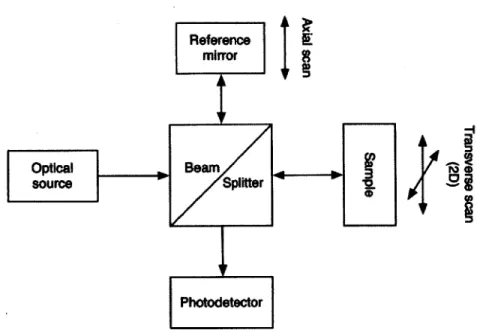
1-2 Block diagram of a simplified OCT system. . . . . 14

1-3 Light scatters off of acoustic wavefronts in an acousto-optic modulator. 19 1-4 Basic OCT signal processing chain. . . . . 24

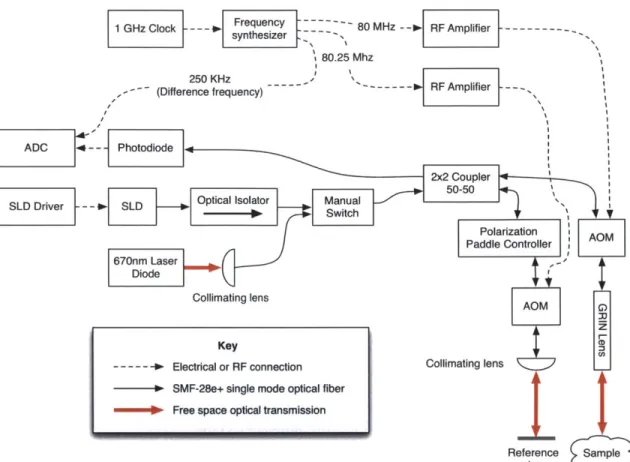
2-1 Block diagram of the FO-DOCM system. . . . . 30

2-2 Schematic of the 1 GHz clock. . . . . 31

2-3 Zemax raytrace simulation of reference path. . . . . 32

2-4 The GRIN lens assembly . . . . 33

2-5 Light lost to an isotropic scatterer, as a function of working distance. 34 2-6 3D model and photograph of the mechanical alignment apparatus. . . 35

2-7 Side view of the alignment apparatus. . . . . 36

2-8 Photograph of the piezo motion stage. . . . . 37

2-9 _{A close up view of the GRIN objective mounting apparatus. . . . . . 38}

2-10 An overview of the digital alignment microscope. . . . . 39

2-11 A raytrace diagram of the microscope layout, simulated in Zemax. . . 40

2-12 The point spread function of the microscope, as simulated in Zemax. 40 2-13 An image of a 1951 USAF Resolution Test Target, captured using the digital m icroscope. . . . . 41

2-14 An image of the visible laser spot on cochlear tissue. . . . . 42

2-15 The transverse X-Y stepper motor stage. . . . . 42

2-16 A block diagram overview of the steps necessary for image generation. 44

2-18 Theoretical axial point spread function. . . . . 46

2-19 A Zemax raytrace showing the path of light through the GRIN lens. . 48 3-1 The measured axial point spread function. . . . . 50

3-2 Result of en-face scan of USAF target. . . . . 51

3-3 Result of scan of the edge of a a glass coverslip. . . . . 52

3-4 Transverse step function measured along the glass coverslip. . . . . . 52

3-5 Noise floor of measured motion. . . . . 53

3-6 Linearity of motion amplitude measurements . . . . 54

3-7 Motion differentiation of adjacent stationary and vibrating interfaces. 55 3-8 An annotated unfixed guinea pig cochlea, imaged with the FO-DOCM system . . . . 56

3-9 A fixed guinea pig cochlea, imaged with the FO-DOCM system. . . . 58

Chapter 1

Introduction

In this chapter, the construction of a fiber optic Doppler optical coherence microscopy system will be motivated. Additionally, the mathematical underpinnings of the sys-tem will be introduced, and recent related work will be discussed.

1.1

Motivations for a fiber optic DOCM system

The mammalian cochlea is capable of remarkable sensory perception. It can distin-guish vibratory motion as small as the radius of a hydrogen atom and discriminate between up to 30 frequencies within a single semitone [10]. However, the mechanics of motion in the inner ear remain poorly understood. The Micromechanics Group at the Research Laboratory of Electronics at MIT is analyzing motion in the cochlea in order to more fully understand what enables these remarkable sensory capabilities.

A tissue of particular interest in the cochlea is the tectorial membrane, which

is in direct contact with the sensory hair cells, as shown in Figure 1-1. This tis-sue's proximity to the hair cells and its interesting mechanical properties, including frequency-sensitive acoustic wave propagation, suggest that it could play an active role in auditory frequency discrimination and motion amplification [11].

A technique known as optical coherence tomography allows three-dimensional

imaging into and through cochlear tissues such as the tectorial membrane by making use of the auto-correlation properties of temporally incoherent light. This technique

Figure 1-1: A schematic drawing of tissues in the cochlea. Adapted from a public

domain image by Oarih Ropshkow.

can image more deeply into tissues than other three-dimensional imaging methods such as confocal microscopy. Furthermore, by measuring the Doppler frequency shift of scattered light, OCT allows for measurement of both constant and periodic mo-tion [5].

The Micromechanics Group at RLE currently uses a free space Doppler optical coherence microscopy system to image the mammalian cochlea and acquire data about the mechanical motions of tissues

[15].

As the FS-DOCM system is designed around free space optics, they must be care-fully aligned and positioned on an optics table. This design has several disadvantages, chiefly that it is difficult and time consuming to align with the animal that is being

imaged. This process takes significant time due to the need to move the animal pre-cisely under the DOCM objective, and the need to align the cochlea with the fixed optical axis of the DOCM system.

The system described in this thesis, while similar in many ways to the existing

FS-DOCM system, primarily uses fiber optic (FO) coupled components. Therefore, it will

be hereafter referred to as the FO-DOCM system. Fiber optics can be more compact and mobile than free space optical components. Additionally, the objective used for imaging the actual tissue is mounted on a custom designed mechanical apparatus that allows the angle and position of the optical axis to be easily adjusted, working with the researcher and research animal, rather than forcing the animal to conform to the optical system. The use of a graded index (GRIN) objective lens, rather than a conventional microscope objective, further reduces the size of the imaging device. These improvements should significantly improve the workflow of other researchers in the Micromechanics Group.

Additionally, the FO-DOCM system uses a longer wavelength of light than the

FS-DOCM system, 1310 nm IR instead of 800 nm IR. While this has some

disad-vantages in axial and transverse resolution capability, as discussed in Section 1.2, this wavelength also has several advantages. It is a commonly used wavelength for communication applications, and therefore many optical components are designed for compatibility in this region. More importantly, 1310 nm has significantly reduced scattering through bone tissue, therefore allowing for greater light transmission and penetration [22] [1]. This has the potential to obviate the current need to image through either the cochlear round window or a hole cut in the cochlear apex.

1.2

_{Principle of operation of time domain OCT}

Throughout this document, the coordinate axis parallel to the direction of light emis-sion from the objective shall be referred to as the "axial" direction, or "z" axis. The plane perpendicular to this axis is known as the "transverse" plane, or, sometimes, the "x" and "y" axes.

Reference E

mirror

I

OptiBeamSplitter

Photodetector

Figure 1-2: Block diagram of a simplified OCT system.

OCT functions by utilizing the principle of the Michelson interferometer. A block

diagram of a significantly simplified OCT system is shown in Figure 1-2. First, light is split into two beams. One beam is reflected from a mirror, and the other beam is scattered from a biological sample. The light is then recombined and the intensity measured by a photodetector. When the optical path lengths of the two beams are closely matched, an interference pattern may be observed. By using temporally inco-herent (broadband) light, the interference pattern is capable of absolute localization, as will now be shown.

The electric field from a temporally incoherent source can be modeled accurately as a wide-sense stationary random process with a power spectral density (PSD) cor-responding to the optical spectrum of the source [2]. In the case where the scattering sample is replaced by a reflecting mirror, the mathematical analysis may be simpli-fied greatly by assuming that the system is measuring the interference of this random process with itself, delayed by the optical path length difference. With these assump-tions, it is shown that the interference pattern is equivalent to the autocorrelation of the random process and may be related to the source PSD [8].

I(t) = IV(t)l2= V*(t)V(t) . (1.1)

In an OCT system, the light from a reference path is combined with the light from a sample path after some delay. This superposition may be expressed as

VD(t; At) -VS(t) + VR(t + At) .

(1.2)

As measuring instantaneous electric field amplitude is impossible, only the ex-pected value, or the time average, of the intensity is of interest, indicated by the notation (x(t)). The time averaged intensity of the superimposed light is

ID(At) = IDt;A)

= (V,3(t; At) VD(t; At))

(1.3)

- (Is(t)) + (IR(t)) + 2 Re(FsR(At ))

where J'xy represents the cross correlation between two random processes X and Y.

The time delay between the two signals, At, is proportional to the path length difference between the two beams, and may be calculated as At = Az/c. When both the sample and reference paths are illuminated from the same light source, the cross correlation function above simplifies into an autocorrelation function of the light source. From here, the Wiener-Khinchin theorem can be applied, which states that the autocorrelation function of a wide-sense stationary random process is

Fxx(T) = 2 Sxx(f) exp(27rjTf)df , (1.4)

straightforwardly related to the process power spectral density Sxx(f) by a Fourier

transform.

Therefore, the axial resolution in an OCT system is limited by the spectral prop-erties of the light source. The width of the envelope of the autocorrelation function, and therefore the axial resolution, is found to be

n

=

1C =

(1.5) _{7w AA}

for a source of center wavelength AO and FWHM bandwidth AA, assuming a Gaussian

PSD [8].

The autocorrelation function also has a periodic interference component, as the

PSD Sxx(f) in Equation 1.5 is not DC biased, but instead is centered around the central optical frequency of the source. In the spatial domain, this represents itself as a carrier wave modulating the autocorrelation envelope, with a spatial period of one wavelength. The time-domain frequency of this carrier as captured by the photodetector,

fmod = 2v,/Ao , (1.6)

is therefore dependent both on the wavelength of the light source, A0, and the speed of

the axial scan, v. [8]. Note that the factor of two results from the fact that changing the length of the reference path by a distance Az changes the optical path length by 2Az.

1.2.1

Limits of transverse resolution

Unlike the axial resolution, the transverse resolution of the optical system is limited

by both the central wavelength of the optical source and the optics used to shape and

focus the light. In the case of the FO-DOCM system, these consist of an objective lens and an optical fiber, which projects light through an air gap onto the lens. The objective lens is a graded index (GRIN) lens, that uses glass with a continuously varying index of refraction to focus the light onto the desired focal point.

Light travels through, and is emitted from, a single mode fiber as a Gaussian beam, a beam of light with a transverse intensity profile approximated by a Gaussian function. A Gaussian beam may also be described by a complex beam parameter q, more easily defined by its inverse

1 _1

= - _{( )}

q(z) R(z) Z rw(z)2 (1.7)

where R(z) is the radius of curvature of the electromagnetic field, and w(z) is the beam radius at a distance z from the beam waist, defined as the transverse distance where intensity has fallen to 1/e2 _{[23]. Therefore, the beam radius may be related to}

the q parameter by

w(z) = .A (1.8)

7r Im(1/q(z))

The transverse resolution of the FO-DOCM system is determined by the minimum spot size of the focused Gaussian beam of light. The evolution of a propagating Gaussian beam may be determined by matrices of the form

a b

(1.9)

c d

referred to as ray transfer matrices, where

Aq(zi) + B

q(z2) Cq= i)+ . (1.10)

Cq(zi) + D

The ray transfer matrix for forward propagation through free space is

(1.11) 0 1)

where 1 is the distance traveled. The ray transfer matrix for a graded index lens is

cos vi Al (no A)-1 sinV\/lA , (1.12)

-(noV ) sin V4iA cos vTA

A

where the refractive index profile of the GRIN lens is n(r) = no(1 - A;2), and the length of the lens is 1 [23].

Therefore, the cascaded ray transfer matrix for the entire system, from fiber emis-sion to a focused spot, is

1 CO1 cos/ 2 (no vA)- Sin VA12 1 13

0 1 -(noVA) sin /A12 cos V12 0 1

'-1+1)o

o(V_1k

cos( - \/A COS2) 1(no sin(v l2) vAV -+t-A-n -l + -113 n.)sin(v/A2

-Ano sin(V74l2) cos(VTl2)- VTAl3no sin( VAl2)

(1.13)

where 13 is the distance from the end of the optical fiber to the GRIN lens, l2 is the

length of the GRIN lens, and l1 is the distance from the end of the GRIN lens to the

focal point. By applying Equation 1.10, the new complex q parameter of the focused beam is

sin(VAl2)(Alin2(l + qo) - 1) - VAno cos(VAl2)(li + 13 + qo)

Ang(l + qo) sin(Vl2) - V'Ano cos(V/Al 2)

where qo is the complex beam parameter at the point of emission from the optical fiber. Using Equation 1.8, and by multiplying by a scale factor, the beam radius can be converted to an expression for the transverse FWHM distance

_ = 2In 2 -A (1.15)

7r Im( 1/qi)

1.3

OCT with acousto-optic modulators

As derived in the previous section, the speed of the z-axis motion defines the frequency of the interferogram carrier. For typical cases, this is on the order of 1 KHz. If the speed of the scan is variable, this carrier is inconsistent, and if the scan stops at a particular point, the frequency is near zero (non-zero only due to spurious mechanical vibration).

In some cases, such as when phase recovery of the carrier frequency signal is nec-essary, as is the case for the FO-DOCM system, it is desirable to have an independent carrier reference. This can also be useful for cases where the z-axis speed is zero, as

in en-face OCT, or when a carrier frequency independent of the speed of the z-axis

scan is desired. One method of accomplishing this is the use of an optical heterodyne, which may be created with acousto-optic modulators (AOMs), also known as Bragg cells [2] [14].

1.3.1

Principle of operation of an AOM

Acoustic absorber

Figure 1-3: Light scatters off of acoustic wavefronts in the quartz crystal of an acousto-optic modulator. As it scatters, it changes both frequency and propagation angle.

Acousto-optic modulators are crystals, typically quartz, that use the acousto-optic effect to shift the frequency of light. A transducer establishes an acoustic standing wave at radio frequencies, typically 40-200 MHz, inside the crystal. Acoustic compression waves in the crystal can be modeled as gradients in the refractive index. Light incident upon these refractive index gradients will be scattered, changing both propagation angle and optical frequency. Momentum conservation of the scattered light requires that the condition

kacoustic + kincident kdiffracted (1.16)

be satisfied by the wave vectors of the acoustic, incident optical, and diffracted optical waves [13].

This can be solved to give a condition on the angle in the case where ki is orthog-onal to k,

sin

0

Ik

--

Ikil nA

with optical wavelength A and acoustic wavelength A. A small angle approximation is applied as it is assumed that Ikjj> ksl.

In some crystals, higher order diffraction angles occur, however, it is difficult to achieve high modulation efficiencies, and they are not of significant interest to this research.

Energy conservation further requires that the frequency of scattered light be shifted by F, the acoustic wave frequency [13]. This frequency shift is what makes

an AOM of practical interest for the creation of an optical heterodyne.

1.3.2

Generating a carrier wave with an AOM

Even with an imprecise or drifting optical center frequency, the precise shift frequency induced by an AOM can be used to generate an extremely stable optical interference signal [14].

The instantaneous complex electric fields for monochromatic plane waves of two different frequencies,

f

Ea(t) = E, exp (27rftj)

Eb(t) = Eb exp (27r(f + F)tj)

The interference between the superposition of these two fields,

Ea(t) + Eb(t) =E, exp (27rftj) + Eb exp (27r(f + F)tj)

=E, exp (27rftj) + Eb(exp (27rftj) exp (27rFtj))

=E, exp (27rftj) (1 + Eb exp (27rFtj)) (1.19)

Ea =Ea(t)(1 + exp (27rFtj)) ,

creates a beat frequency, with the amplitude of the optical frequency modulated by the slower, and detectable radio frequency F.

For many applications, the radio frequency F used to drive the AOMs is a higher frequency carrier than is desired or can be detected. In this case, it is possible to use two AOMs to generate an even lower frequency carrier by driving them each at slightly different frequencies, resulting in complex field amplitudes

Ea(t) = Ea exp (27rtj(f + F1)) (1.20)

Eb(t) = Eb exp (27rtj(f + F2))

It can be seen via an identical simplification to the above that the combination of these electric field amplitudes creates a carrier wave with frequency equal to the absolute value of F - F2.

1.4

Doppler OCT with AOMs

Optical scattering from moving particles also induces a change in the frequency of scattered light due to the Doppler effect. This change in frequency can be expressed as

Af~~~~ (t =f ₂v = )

fo

c 2 (.1

where a is the angle between the direction of incident light propagation and the light detector, 3 is the angle between the direction of light propagation and the direction of motion of the media, and v(t) is the instantaneous velocity of the sample [6].

In the FO-DOCM apparatus, only backscattered light can be detected, so a is assumed to be 7r radians. The direction of motion is assumed to be in the direction of light propagation for simplicity, so that

#

frequency change then simplifies to

Af (t) - ₂v(t)

fo

Integrating the instantaneous frequency finds the phase, up to a constant term, as

(t) =

J

= 27r fo(1 + 2 )dt (1.23)

= 27r

ft

where d(t) is the instantaneous sample displacement, the integral of the sample ve-locity.

In an analogous way to Equation 1.18, instantaneous field amplitudes E, and Eb,

representing the sample and reference paths respectively, may be written as

Ea(t) = E, exp 27rj(f + 2F1) t + 2d(t)

c (1.24)

Eb(t) = Eb exp (27rtj(f + 2F2)) ,

where Ea has scattered from media moving with velocity v(t) and has passed through an AOM of frequency F1, while Eb has been reflected from a stationary object and

has passed through an AOM of frequency F. Note that the radio frequencies F and

F2 have been multiplied by two, as light must make two passes through each AOM.

The electric field at the detector is the sum of the two electric field amplitudes,

Eb(t) + Ea(t) = E, exp (27rtj(f + 2F₁)) (exp (27rj (f + 2F1)) (1.25)

+

K

This equation may be simplified slightly to

Eb(t) + Ea(t) = Ea exp (27rtjf') exp 27rjf' 2d(t) + exp (-27rtj2AF)) (1.26)

by substituting two new symbols for the modified optical frequency,

f'

The instantaneous light intensity is equivalent to the absolute value of the instan-taneous electric field amplitude squared, given by

I(t) = _{E2 + Eb + 2EbE, cos 27r 2tAF + f'} . (1.27)

The result of the frequency shift induced by the motion of the media can clearly be seen in the instantaneous phase of the intensity oscillation,

2d(t )

0(t) = 27r (2tAF + f' . (1.28)

This is equivalent to phase modulation, with the periodic change in phase of

27rf' . (1.29)

This oscillation can be extracted from the captured signal using the Hilbert trans-form, discussed in Section 1.5.1. While this derivation assumed perfectly monochro-matic light sources, as would be the case in an ideal laser interferometer, the result also generalizes to the non-monochromatic random signals used in Section 1.2.

1.5

Signal processing

Photodetector Arplifier Analog band pass filter Analog to digital

converter

Digital band pass _Downsampling

filter exrcto

Figure 1-4: Basic OCT signal processing chain. The bandpass filter is centered around the carrier frequency from Equation 1.6. The demodulator can be either as straight-forward as an envelope follower or a Hilbert transform based analytic continuation.

Figure 1-4. After detection of the light and signal amplification, but prior to analog-to-digital conversion, analog bandpass filters select for the carrier frequency and its sidebands, in addition to bandlimiting the signal below the Nyquist frequency. The signal is then sampled and quantized by an ADC so that it may be manipulated digitally.

The Hilbert transform can then be used to extract the envelope from the modu-lated carrier signal. Assuming a signal of the following form,

x(t) = A(t) cos (wt) , (1.30)

the Hilbert transform can generate the approximate quadrature component,

H(x(t)) ~ A(t) sin (wt) , (1.31)

where A(t) is a real envelope [19].

It can therefore be seen that the envelope component of the signal can be calcu-lated as

A(t) ~

/(x(t))

The envelope, which does need the high sampling rate previously required in order to capture the carrier frequency, can then be low pass filtered and decimated to the

resolution required by the imaging application.

Additionally, it can be seen that the instantaneous phase of this arbitrary sinu-soidal signal may also be estimated using the Hilbert transform as

0(t) ~ tan-' H(x(t)) . (1.33)

(X (t)

1.5.1

Analyzing motion

As shown in Section 1.4, the phase of the modulated light intensity scattered from moving media, referred to as the heterodyne phase,

#het,

Ohet(t) = 27r 2tAF + f' 2d(t) . (1.34) A reference signal must also be captured, which oscillates at a frequency equal to

the difference of the two RF drive frequencies. The phase of this reference is

Oref (t) = 27rtAF , (1.35)

exactly half the phase of the carrier frequency of the heterodyne signal.

Subtracting twice the reference phase from the heterodyne phase, and replacing c

by c/n to account for the refractive index of the media, finds the phase difference

#dif(t)

c/n)

Because the RF frequency F <<

f,

f

f

f,

as a wavenumber k further simplifies the phase difference to

kdif (t) 2rtf 2d(t) 2knd(t) . (1.37)

c/n

Using the result from Equation 1.33, the instantaneous phase difference between the captured heterodyne signal, Vhet, and the captured reference signal Kef, may be written as

Odif (t) r.,tan- 1 (HVe~) - 2 tan- .(rf() (1.38)

Vhet (t) (Vref (t)

Combining Equations 1.37 and 1.38, the periodic displacement of the sample may be calculated as

e1 (tan-i H(Vhet)(t) 2 tan- H(Vre )(t) (1.39)

1.6

Related work

Since the 1960s, interferometry with laser light has been used to measure vibration in the cochlea. Early laser Doppler interferometer experiments required the placement of reflective beads to isolate tissues of interest; however, these beads can influence the mechanical properties of the cochlea [18]. Recent methods involving laser Doppler interferometry have had success in measuring vibrations with a noise floor as low as

30 pm/Hz0.5 without beads, but also require a parallel system, such as confocal

mi-croscopy, in order to produce an image of the tissues [16] [20] [21] . Furthermore, laser interferometers are highly coherent, so without reflective beads, vibration measure-ments have a depth separation determined primarily by the beam divergence angle, resulting in poor axial isolation.

Low coherence interferometry, such as OCT, is capable of solving these problems. As mentioned in Section 1.1, the FO-DOCM system is designed to update the previous free space system used in the Micromechanics Group. The FO-DOCM system is quite similar to the FS-DOCM system, but is also different in several ways: the use of fiber optic components rather than free space optics, the use of a longer wavelength source, and the revised alignment and positioning apparatus [15]. Furthermore, the FO-DOCM system allows for continuous scanning of lines in an image in addition to point-by-point pixel acquisition.

Other time-domain Doppler OCT systems. The use of acousto-optic

modula-tors is not essential for Doppler OCT, and systems similar to the FO-DOCM system have been constructed without them. However, without a reference signal to use in extracting phase modulation information, the system responds to vibration ampli-tude in a very non-linear way. Furthermore, because vibrations are not modulated to higher frequencies by the heterodyne carrier, more interference at low frequencies, from mechanical vibrations and electrical 1/f noise, results in a higher noise floor, typically on the order of 30 pm/Hz0_.5 _[3].

Spectral-domain Doppler OCT systems. While the FO-DOCM project uses time-domain Doppler OCT, work has also been done in the field of spectral domain Doppler OCT. Spectral-domain Doppler OCT systems have achieved results with an axial resolution of 13 pm and a motion detection noise floor of 300 pm/Hz0 5 _{[4] [24].}

It is thought that a time domain approach can result in higher resolution motion measurements than a spectral domain system, as monolithic photodiodes have better noise equivalent power than a CCD line camera with a diffraction grating. Further-more, the sampling rate of a CCD sensor is very limited compared to a photodiode, restricting the speed and accuracy of phase recovery between sequential scans. How-ever, the use of a time-domain system adds the considerable expense of requiring physical motion to scan the z-axis, resulting in significantly slower image acquisition.

Trans-bone imaging. Doppler OCT has previously been used with some success

for measuring vibrations of cochlear tissues through bone. Using a 935 nm center wavelength, motion inside an in vivo mouse cochlea was measured with an noise floor

of approximately 100 pm/Hz0_-5

[9]. It is suspected that a 1310 nm center wavelength,

as used in the FO-DOCM system, will be even more effective at penetrating bony tissue [22] [1].

Microangiography. Doppler OCT is not restricted to measuring periodic

vibra-tions - one of its first applications was for angiography, measuring the velocity of blood flow inside tissue. Current techniques with Doppler optical microangiography are capable of isolating and measuring blood flow in a single vessel over time [7]. While low frequency motion, such as constant motion, has a significantly higher mea-surement noise floor, blood flow velocity amplitudes are also typically much greater than vibrational amplitudes.

Miniaturization of OCT apparatus One of the advantages of the FO-DOCM

system to the Micromechanics Group is its smaller size, so this work may be seen as continuing the active effort of minimizing the size of OCT apparatuses. Research in this area includes the creation of a miniature swept frequency laser source for OCT

imaging [12], which could enable a higher axial resolution in a smaller form factor. GRIN lenses, used in the FO-DOCM system, have a significant size advantage in addition to high quality optical performance and have also been used in previous research as endoscopic probes for OCT [25].

Overall, the FO-DOCM- system designed and constructed in this thesis builds on previous work and ideas in optical coherence tomography to develop an apparatus that satisfies the unique set of requirements of the Micromechanics Group, with advantages

Chapter 2

System design

In this chapter, the major components of the fiber optic Doppler optical coherence microscopy (FO-DOCM) system will be introduced, and the constraints that led to their choice will be examined. The mechanical and optical design will be detailed. Finally, predictions of system performance will be made based on component choices.

2.1

System overview

2.1.1

Incoherent light source

The choice of a light source dictates many aspects of the system performance. The coherence length, as shown in Section 1.2, controls the axial resolution of the imaging. The center wavelength of the source constrains the tissue penetration depth, and what other components may be used in the system.

For this project, a super-luminescent diode, or SLD, was chosen (Exalos AG, Switzerland, Part No: EXS210045-01). Super luminescent diodes provide the spatial coherence of a laser with the short temporal coherence of an LED or "white" light source. Other common broadband light sources for OCT applications include solid-state lasers, such as Ti: A1203 lasers, lasers that sweep a frequency range in time (so

called "swept-spectrum" lasers), and femtosecond lasers. The chief advantage of an

1 GHz Clock --- - hesz 80 MHz IF Amplifier ---

---80.25 Mhz

250 KHz - --- RF

-- (Difference frequency) - '

ARFAplifiere---ADC -- Photodiode

Wx Coupler

SLD Driver -- -JSLD Optical Isolator Manual

670n Lasr SwtchPolarization Paddle Controller AOM Diode

Collimating lens

AOM

Key

--- -4 Electrical or RF connection Collimating lens

lo SMF-28e+ single mode optical fiber

40- Free space optical transmission

Reference Sample

mirror

Figure 2-1: Block diagram of the FO-DOCM system.

A center wavelength of 1310 nm was chosen as this is a common wavelength

for communications. It is therefore possible to find many inexpensive fiber coupled components designed to operate in this band. Additionally, as discussed in Section

1.1, a longer wavelength could allow for deeper penetration through the bony cochlear

wall [22] [1].

An optical isolator is required after the SLD in order to prevent back reflections from resonating and adversely impacting the spectral bandwidth of the source.

2.1.2

Acousto-optic modulators

Two fiber coupled acousto-optic modulators (Gooch & Housego, United Kingdom; packaged by Sintec Optronics, Singapore. Part No: 23080-1-1.3-LTD-FC/APC) were chosen, which provide a convenient, compact device and avoid the need for alignment with the first degree deflection beam, required in free space optics. An 80 MHz drive

frequency was chosen for compatibility with existing hardware used in the Microme-chanics Group.

2.1.3

RF generation and driving

The AOMs must be driven by an 80 MHz and an 80.25 MHz RF signal in order to produce the beat frequency derived in Section 1.3.2. A frequency synthesizer, built

by former Micromechanics Group student Stanley Hong

[15],

source to synthesize a 80.25 MHz signal and an 80 MHz signal. The mixed difference between these signals, a 250 KHz reference signal, is also generated, as it is necessary for later signal processing steps.

Two RF amplifiers, (Mini Circuits, United States. Part No: ZHL-3A) amplify the RF signals +29.5 dBm to +32 dBm (approximately 1.5 watts), the maximum drive power of the AOMs.

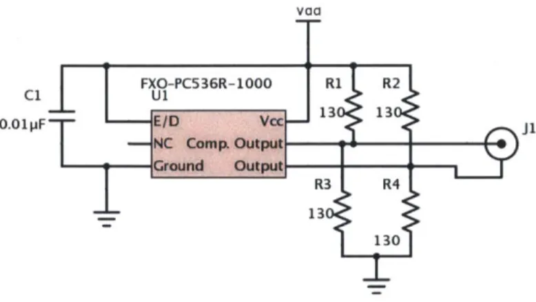
The 1 GHz clock is generated by a small integrated oscillator (Fox Electronics, United States. Part No: FXOPC536R-1000). An output of +13 dBm was measured at 50Q, sufficient for driving the frequency synthesizer. This oscillator and the small amount of supporting electrical hardware required was packaged in an enclosure and connected to a BNC output. vaa C1FXO-PC536R-1000 R1 R2 0.01pF # E/D Voc 13 1 NC Comp. Output Ground _Output R3 R4 13 130

2.1.4

Reference path

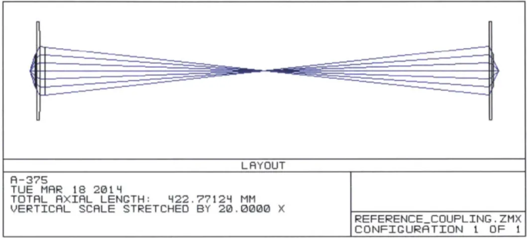
The reference path uses an adjustable focus fiber optic coupled collimator, and focuses it onto a mounted aluminum front surface mirror. A mirror was used instead of a retroreflector as its greater parallelism resulted in higher coupling efficiency than was achievable with a retroreflector, despite the increased difficulty in alignment. The collimator was used with an FC/APC fiber optic terminator in order to reduce back reflections. This setup was simulated with Zemax optical design software, as shown in Figure 2-3, predicting a single mode fiber coupling efficiency of -0.55 dB.

LAYOUT

R-375

TUE MAR 18 2014

TOTAL AXIAL LENGTH: 422.77124 MM VERTICAL SCALE STRETCHED BY 20000 X

REFERENCECOUPLING. ZMX CONFIGURATION I OF 1

Figure 2-3: Zemax raytrace simulation of reference path. Note that the vertical axis is enlarged by 20x, and that the mirror is represented by duplicating and reversing the optical system about the center.

The mirror was mounted on a non-motorized, single axis micropositioning stage, allowing the reference path length to be adjusted so that it matches the distance to the sample path objective focal point.

2.1.5

Sample path objective

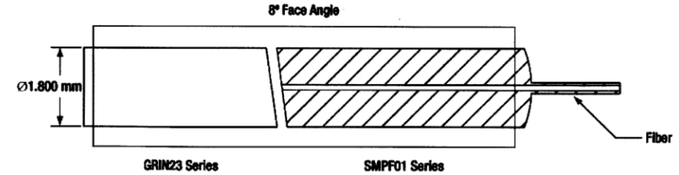
A graded index (GRIN) lens (Thorlabs, United States. Part No: GRIN2313A) was

used to focus light onto the sample under examination. The GRIN lens is sold as a package that can be assembled to focus to a desired distance. An 8 degree angled face is used to reduce back-reflection. This was fixed in place with a UV cured optical adhesive (Norland Products, United States. Part No: NOA68).

r*Face Angle

01.800 MM

Fiber

GRIN23 Series SMPFO1 Series

Figure 2-4: The GRIN lens assembly. Adapted from an image by Thorlabs. The physical distance from the GRIN objective lens to the sample under exam-ination, referred to as the working distance (W), is determined by balancing the achievable penetration depth, the amplitude of scattered light, the transverse resolu-tion, and the complexity of positioning the lens near the sample.

The solid angle Q subtended by the GRIN lens is equal to

Q = 27r(1 - cos 0) , (2.1)

where 6 = arctan r , or equivalently,

Q = 27r 1 - W2 (2.2)

W2+ r2ri

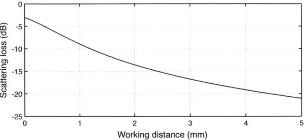
Assuming an isotropic scatterer, the fraction of optical power that will be recol-lected by the GRIN lens is equal to -. As the GRIN lens used in this thesis has a radius of 0.9 mm, this fraction may be written numerically as

1 W2

- 1

-.(2.3)

2 W2 +0.81)

A plot of this scattering loss for working distances between 0 and 5 mm is shown

in Figure 2-5.

A working distance of approximately 2.5 mm was chosen, as it provided the

min-imum sufficient distance between the lens and sample, while avoiding unnecessary scattering loss or resolution limitations.

0 U) 0 0) U) -5 0 1 2 3 4 5 Working distance (mm)

Figure 2-5: Light lost to an isotropic scatterer, as a function of working distance.

2.2

Sample alignment apparatus

The sample alignment apparatus, pictured in Figure 2-6, is a mechanical device de-signed to accomplish several goals:

* Securely hold the GRIN objective lens

" Move the GRIN objective along the direction of the optical axis with a precise motorized stage

" Allow the GRIN objective lens to be rotated a certain angle around its focal point

" Allow adjustments for height and horizontal distance

" Provide a visible alignment aid beam

" Hold a small digital microscope for visual inspection of alignment

2.2.1

Mechanical device for adjusting angle and position

I

-10 -15

-20

/

4

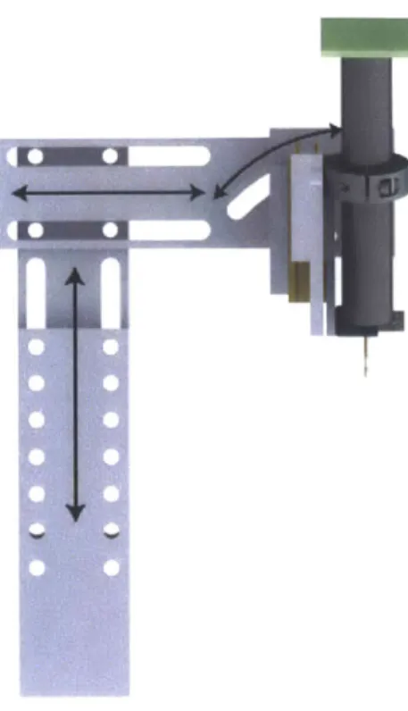
Figure 2-6: A 3D model and a photograph of the mechanical alignment apparatus.

1) Vertical adjustment slider. 2) Horizontal adjustment slider. 3) Angular

adjust-ment slider. 4) GRIN objective lens. 5) Z-axis piezo stage. 6) Digital microscope.

F

I

Figure 2-7: Side view of the alignment apparatus, with arrows indicating mechanisms for adjusting position and angle.

able to change the angle of axial movement without changing the current focal point, a helpful feature for alignment.

The cantilever part was designed in SolidWorks and then milled on a CNC machine in the Edgerton Center Student Shop. An 'L'-shaped part was designed to hold the horizontal cantilever. Later, a vertical part was added to enable continuous adjustment of cantilever height and to allow for a higher maximum height, necessary as a result of the clearance requirements of the 2D transverse stage. These parts were milled by hand at the Edgerton Center Student Shop.

2.2.2

Piezo motor stage for axial movement

To control z-axis scanning, a piezo-electric motorized stage was used (Newport, Inc., United States. Part No: CONEX-AG-LS25-27P). This stage uses an "inchworm" drive method to control motion in discrete steps. Quadrature position encoders with closed loop feedback provide movements repeatable of up to a manufacturer

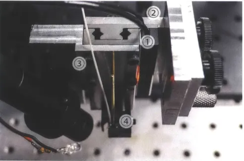
Figure 2-8: A photograph of the piezo motion stage. 1) Piezoelectric motorized stage. 2) 'L'-backet to mount piezo stage. 3) 'S'-bracket to mount GRIN lens. 4) GRIN lens 'V'-clamp.

Unfortunately, this stage also has some drawbacks for an OCT application. Though the closed loop feedback allows for the stage to move precisely to any location, the speed of movement is not consistent. As a result, it is necessary to either collect data pixel-by-pixel or to re-interpolate the data collected based on the actual posi-tion of the stage as it scans. These methods, and their advantages and drawbacks, are discussed further in the signal processing section, Section 2.5.

To capture information about the real time position of the stage, two approaches were used. The first involved repeatedly querying the stage driver over a serial con-nection. While this was straightforward to accomplish and within the bounds of normal operation of the stage, it (lid not provide high enough time resolution of the position of the stage. The second approach required adding analog output from

the stage encoders that could be captured directly by the analog-to-digital converter simultaneously with the interferoinetric signal. This involved extracting the quadra-ture encoder signal from the controller circuit board and soldering additional BNC outputs.

a custom mounting bracket designed for the unique hole spacing on the stage. The bracket is also designed as an 'L' shape, so that the GRIN lens points in the radial direction of the angle adjustment arc.

2.2.3

Mounting the fiber and GRIN lens

Figure 2-9: A close up view of the GRIN objective mounting apparatus. 1) GRIN objective. 2) Brass extension rod used to lower the GRIN lens. 3) V-clamp. 4) Digital microscope. 5) Optical fiber (truncated in image.) 6) 'S' bracket.

To hold the GRIN lens at a sufficient distance from the stage with minimal bulk, a small brass rod was adhered with a UV-cured optical adhesive to the outer glass tube in the GRIN lens assembly. A V-clamp was used to firmly hold the brass rod in place. A custom 'S'-shaped mounting bracket was designed and milled to connect to the piezo stage, allow the V-clamp to be mounted, and also to allow the digital microscope to be installed such that it could image the focal point of the GRIN lens. Note that without the brass extension rod, the focal point of the GRIN lens would be blocked from the view of the microscope by the V-clamp and supporting hardware. The narrow profile of the brass tube and GRIN lens also allow the objective to be positioned more easily near the sample under examination.

2.2.4 Digital microscope for visual alignment

Figure 2-10: An overview of the digital alignment microscope. 1) LED illumination source. 2) Mounting bracket (position and angle adjustment). 3) Lens tube. 4) USB web camera CCD.

In order to aid the alignment process, an optical microscope with a digital CCD viewfinder was constructed to observe the region imaged by the OCT process.

The design required a relatively large working distance, and correspondingly low numerical aperture, in order to allow the microscope to have an angle as close to the optical axis of the OCT objective lens as possible.

A CCD sensor from a USB web camera (Microsoft, United States. Part No: Xbox Live Vision) was used, due to its compact size, low cost, and use of the standard USB Video Class protocol, compatible with MATLAB and other image capture applica-tions. As the CCD has a quite small size, approximately 3x5mmn (actual dimension specifications are not available), a low magnification was sufficient.

A MATLAB script was used to optimize the working distance using a simple paraxial lens approximation, while keeping the overall optical length within reasonable limits, and while working with a set of easily obtainable lenses. From this MATLAB program, a Zemax simulation model was created, using accurate models of the real lenses from which the microscope would be constructed.

The microscope is composed of three lenses in two groups: a 15 mm1 spherical doublet (Edmund Optics, United States. Part No: 45209) and a 20 mm spherical singlet (Thorlabs, United States. Part No: LA1074). The lenses are mounted in a 1/2 inch diameter lens tube. A 4 mn diameter aperture, laser cut from opaque

acrylic, was used to further reduce spherical aberrations, improving image quality at the expense of light intensity. A raytrace diagram of the microscope is shown in Figure 2-11, and the predicted point spread function in Figure 2-12.

TUE MAR 25 2014

TOTAL AXIAL LENGTH: 159,72000 MM VERTICAL SCALE STRETCHED BY 5.0000 X

I

LAYOUT

MICROSCOPE ' ZMX

CONFIGURRTION I OF L

Figure 2-11: A raytrace diagram of the microscope layout, simulated in Zemax.

-9 0 P X-POSITIDN IN Pm 16 24 32 V PSF CROSS SECTION MICROSCOPE. ZMX CONFIGURATION I OF I

Figure 2-12: The point spread function of the microscope, as simulated in Zemax.

The performance was tested by imaging a backlit 1951 USAF Resolution Test Target, demonstrating that the microscope is capable of resolving features as small as 7.8 pm wide, and has a field of view of 1.16 mm x 0.87 mm, for a magnification of approximately 4x. 9 8.2 0.3 TUE MAR 25 2019 FIELI 0 L M WRVE=LENGTH:0POLYOIROMRTIC LIN X SECTION, CENTER ROW.

Figure 2-13: An image of a 1951 USAF Resolution Test Target, captured using the digital microscope.

Due to the nature of the microscope's intended application, the sample is not illuminated by transillumination but instead by viewing the light scattered by the sample from a bright LED source mounted near the end of the microscope. While the performance of this microscope is too limited for most imaging applications (in particular, the contrast is quite poor, as evidenced by the "haze" around the bright regions in Figure 2-13), it is sufficient for performing basic alignment of the

FO-DOCM system and is therefore sufficient for the system design requirements.

2.2.5

Visible laser for assisting visual alignment

The spectral responsivity of a silicon photosensor, like that used in the digital mi-croscope CCD, falls sharply above 1000 nm. As the optical source in this system is centered at 1310 nm, it is difficult to view the spot produced by the focused infrared light. To solve this, a second optical source can be coupled into the GRIN lens.

For this purpose, an inexpensive 650 nm laser diode is used. The output of the diode is collimated and coupled into an optical fiber, which can be attached through an FC/APC connector directly to the GRIN lens. This produces a highly visible laser spot that is helpful for aligning the start of an OCT scan.

Figure 2-14: An image of the visible laser spot on cochlear tissue, captured by the digital microscope.

2.3

X-Y

stage

for sample movement

Figure 2-15: The transverse X-Y stepper motor stage. form, with aluminum stand-offs. 2) Prior H101 two-axis plate.

1) Laser-cut mounting plat-stage. 3) Laser-cut mounting

To move in the transverse plane, the sample is placed on a stepper motor driven two axis stage (Prior Scientific Ltd., Japan. Part No: H101BX), pictured in Figure

2-15. While this stage is designed for use with a conventional upright microscope,

custom mounting hardware was designed and fabricated to allow it to stand freely. The stage is driven by a stepper controller, which accepts commands over a serial connection (Prior Scientific Ltd., Japan. Part No: H128V). The stage has a 1 im step size, but poor repeatability, making it suitable only for 2D scanning in the x-z or y-z planes.

2.4

Light detection and signal acquisition

The light is detected by a photodiode with an integrated transconductance amplifier (New Focus, Inc., United States. Part No: 2117-FC). This photodetector has a sensitivity range of 800-1700 nm and a transimpedance gain of up to 18.8 x 106 V/A, with responsivity near 1A/W at 1310 nm.

As the interference carrier signal is set at 500 KHz, the analog photodiode low-pass and high-low-pass filters in the photodetector are configured to low-pass signals between

300 KHz and 1 MHz.

The output from the photodiode is digitized by using a two input PCI DAC/ADC card (Interface Co., Japan. Part No: PCI-3525). Multiple DAC/ADC cards are daisy chained together to be able to capture greater than two signals simultaneously. This is useful, as up to five signals may be of interest to capture: the photodiode output, the RF synthesizer difference frequency, the acoustic stimulus signal, and the two z-stage quadrature encoders.

To capture these signals, a program was written in C to communicate with the

DAC/ADC. As the photodiode filters frequencies above 1 MHz, a sampling frequency

of 2.5 MHz was chosen to avoid frequency aliasing. The capture program allows for application-specific flexibility and may be used with imaging interfaces in MATLAB and Python.

2.5

Signal processing

The FO-DOCM system is capable of performing two distinct tasks. The first is image generation, where a static 2D or 3D image of the sample is made. The second is motion analysis, capturing information about the movement of one specific area of a sample. The primary difference between these two tasks is that motion analysis requires a segment of data to be sampled from one stationary point while image generation can use a continually scanning axis.

2.5.1

Image generation

An overview of the signal processing steps necessary for continuous scan image gen-eration from acquired data, for a single z-axis sweep, is shown in Figure 2-16.

Digital BPF _{Hilbert transform}

extract thioe envelope oftesga.Uigdtrmtexuaratur n coesoh

signalI

z-a is tago e i sri t ro Position reinterpolation encoder signal

I Decirmation

Figure 2-16: A block diagram overview of the steps necessary for image generation.

First, the captured signal is bandpassed using a digital FIR filter with a smaller passband than is practical with analog filters. Next, the Hilbert transform is used to extract the envelope of the signal. Using data from the quadrature encoders of the z-axis stage, this envelope is reinterpolated to be a function of space instead of time.

As the envelope is much more slowly varying than the original 500 KHz signal, it can be decimated to the size desired for the final image. This process is repeated for each captured line to assemble the full 2D or 3D image. A function to implement these steps was written in MATLAB.

2.5.2

Motion analysis

An overview of the signal processing steps necessary to perform on acquired data to estimate motion parameters, for a single pixel, is shown in Figure 2-17.

--- Fibr tasfr l + Cosine fit - Scaling 10

Interference BPF phase extractionMotion

signal parameters

Digital Hilbert transform x(2

RF synthesizer BPF phase extraction x (-2)

reference

Figure 2-17: A block diagram overview of the steps necessary for motion analysis. This process is the same as that derived mathematically in Section 1.5.1. First, the Hilbert transform is used to estimate the instantaneous phase of the photodiode interference signal, and of the 250 KHz reference output from the RF synthesizer. The difference between the 500 KHz phase signal and twice the 250 KHz phase signal is periodically varying when the phase of the 500 KHz signal varies periodically, as is the case when light is scattered from a moving sample excited at a known frequency.

A sinusoid of this known frequency is fit by linear least squares to this periodically

varying phase, as a noise-resistant method of estimating both the amplitude and the phase offset of the oscillation. This process provides an estimate of the motion parameters at a single point in the sample and can be repeated for as many points are desired, or for an entire array of points, in order to generate an image of motion amplitude and phase in a sample. This analysis is also implemented as a function in MATLAB.

2.6

Theoretical performance predictions

2.6.1

Axial resolution

Axial resolution is limited by the coherence length of the optical source, derived in Equation 1.5 in Chapter 1 as

21n2 A 2

6Z = 1C = . (2.4)

7r A

The specifications for the optical source used in this project were not precisely equivalent to the measured performance of the actual source. The actual -3dB band-width was 86.3 nm, whereas the specified bandband-width was 100 nm. Additionally, the actual power output was 7.00 mW, whereas the specified power was 10 mW. The slightly smaller bandwidth results in an axial resolution of 9.94 Jrm, inferior to the prediction in Section 1.2. The optical spectrum measurements also showed that bandwidth, and therefore resolution, is not adversely impacted by any other optical

components in the system.

From the optical power spectral density, the point spread function can be numeri-cally predicted by calculating the Fourier transform, as derived in Section 1.2. Using the Discrete Fourier Transform, the measured optical spectrum analyzer results may be used to estimate the axial point spread function. The result of this analysis is shown in Figure 2-18. C C E 1 0.9 0.8 0.7 0.6 0.5 0.4 0.3 0.2 0.1 -25 -20 -15 -10 -5 0 5 Distance (pm)

Figure 2-18: Theoretical axial point spread function. trum analyzer measurements of the SLD source.

10 15 20 25

Computed from optical