Data processing and inference methods for zero knowledge nuclear disarmament

Data Processing and Inference Methods for Zero

Knowledge Nuclear Disarmament

by

William DeMaio

Submitted to the Department of Nuclear Science and Engineering

in partial fulfillment of the requirements for the degree of

Bachelor of Science in Nuclear Science and Engineering

at the

MASSACHUSETTS INSTITUTE OF TECHNOLOGY

June 2016

c

○

Massachusetts Institute of Technology 2016. All rights reserved.

Author . . . .

Department of Nuclear Science and Engineering

May 19, 2016

Certified by. . . .

R. Scott Kemp

Norman C. Rasmussen Assistant Professor of Nuclear Science and

Engineering

Thesis Supervisor

Accepted by . . . .

Michael P. Short

Assistant Professor of Nuclear Science and Engineering

Chairman, Department Committee on Undergraduate Theses

Data Processing and Inference Methods for Zero Knowledge

Nuclear Disarmament

by

William DeMaio

Submitted to the Department of Nuclear Science and Engineering on May 19, 2016, in partial fulfillment of the

requirements for the degree of

Bachelor of Science in Nuclear Science and Engineering

Abstract

It is hoped that future nuclear arms control treaties will call for the dismantlement of stored nuclear warheads. To make the authenticated decommissioning of nuclear weapons agreeable, methods must be developed to validate the structure and com-position of nuclear warheads without it being possible to gain knowledge about these attributes. Nuclear resonance fluorescence (NRF) imaging potentially enables the physically-encrypted verification of nuclear weapons in a manner that would meet treaty requirements. This thesis examines the physics behind NRF, develops tools for processing resonance data, establishes methodologies for simulating information gain during warhead verification, and tests potential inference processes. The in-fluence of several inference parameters are characterized, and success is shown in predicting the properties of an encrypting foil and the thickness of a warhead in a one-dimensional verification scenario.

Thesis Supervisor: R. Scott Kemp

Acknowledgments

Firstly, I’d like to thank my advisor and mentor, Professor R. Scott Kemp, for the opportunity to work on this fascinating project, as well as his continuous support, invaluable advice, and ceaseless encouragement. Throughout my time here, he has reassured me through uncertainty, helped me learn to focus my talents, and been a principled role model to whom I aspire.

Secondly, this work would not have been possible without Ruaridh Macdonald. Much of this project is the result of his vision, and his immense contributions of time, guidance, and attention have been instrumental in producing the meaningful work it contains. I am also truly grateful for his friendship.

Additionally, it has been a genuine pleasure to work with everyone in the Depart-ment of Nuclear Science and Engineering. Every student, faculty, and staff member I have worked with has inspired me with their endeavors and thoughtfulness.

Ultimately, my family and friends must be thanked for their endless support. It is thanks to them that I have been able to learn and grow throughout my life, and I am excited and honored to continue on with their enduring love and encouragement. Thank you,

Contents

1 Introduction 13

2 Background 15

2.1 Nuclear Arms Control . . . 15

2.1.1 Overview of Arms Control . . . 15

2.1.2 Demand for Zero Knowledge Methods . . . 16

2.1.3 A Proposed Zero Knowledge Verification System . . . 17

2.2 Nuclear Resonance Fluorescence . . . 17

2.2.1 Resonant States . . . 18

2.2.2 Nuclear Resonance Fluorescence Cross Sections . . . 19

2.2.2.1 Excitation Cross Section . . . 19

2.2.2.2 Integrated Cross Section . . . 20

2.2.2.3 Angular Dependence . . . 20

2.2.2.4 Doppler Broadening . . . 20

2.2.2.5 Recoil Energy and Lattice Effects . . . 22

2.2.3 Inferring Warhead Properties . . . 24

2.2.3.1 Benefits of Analyzing Peaks . . . 24

2.2.3.2 Glass Equation . . . 25

2.2.3.3 Branched Peaks . . . 27

2.2.3.4 Neighboring Peaks . . . 27

2.2.3.5 Overview of Bayesian Methods . . . 28

3 Methodology 31 3.1 Data Processing and Manipulation . . . 31

3.1.1 Data Sources and Pre-processing . . . 31

3.1.2 Functionality . . . 34

3.1.2.1 Computation . . . 34

3.1.2.2 Plotting . . . 34

3.2 Bayesian Inference of Foil Properties . . . 35

3.2.1 Objectives . . . 35

3.2.1.1 Modeling Uncertainty and Knowledge Gain . . . 35

3.2.1.2 Verification of Theoretical Model of Inference . . . . 37

3.2.2 Implementation . . . 37

3.2.2.1 High Level Organization . . . 37

3.2.2.2 Data Processing and Initial Conditions . . . 38

3.2.2.3 Bayesian Update Algorithm . . . 39

3.2.2.4 Challenges . . . 40

3.2.2.5 Solutions . . . 40

4 Results 43 4.1 Testing . . . 43

4.1.1 Overall Performance . . . 43

4.1.2 Effects of Initial Conditions and Variables . . . 47

4.1.2.1 Source Strength . . . 47

4.1.2.2 Gaussian Delta Value . . . 49

4.1.2.3 Guess Intervals and Foil Thickness . . . 52

4.1.2.4 Isotopic Considerations . . . 54

4.2 Scenario Analysis . . . 57

4.2.1 Testing Parameters and the Black Sea Warhead . . . 57

4.2.2 Properties Inferred . . . 57

5 Discussion 61 5.1 Conclusions . . . 61

List of Figures

2-1 Schematic of a proposed verification setup. . . 18

2-2 Level diagram of branched and neighboring NRF peaks . . . 25

3-1 Definition and usage of the EnergyData function. . . 32

3-2 Output of EnergyDataTable for Pu239. . . 33

3-3 Definition and usage of the GatherEnergyLevels function. . . 33

3-4 Definition and usage of the PureAbsorptionCrossSection function. . . 35

3-5 Usage of the BuildPlots function. . . 36

3-6 Usage of the PlotIntegratedCrossSections function. . . 36

3-7 Definition of the NRFGamma class . . . 38

3-8 Organization of the probsFoilHistory matrix . . . 40

3-9 Implementation of the Bayesian update algorithm . . . 40

4-1 Development of thickness estimates with successive peak pairs . . . . 44

4-2 Convergence of probability distributions . . . 44

4-3 Determination of number densities for multiple isotopes . . . 45

4-4 Example of a non-convergent solution . . . 45

4-5 Non-convergent Bayesian priors . . . 46

4-6 Convergence with modified initial probability distributions . . . 46

4-7 Effect of the source strength parameter on number density inference in the foil . . . 48

4-8 Effect of the source strength parameter on inference of foil thickness . 49 4-9 Effect of the source strength parameter on inference of warhead thickness 49 4-10 Source strength summary plot . . . 50

4-11 Comparison of convergence with high and low ∆ parameters . . . 51

4-12 Effect of the Gaussian ∆ parameter on inference of foil composition . 51 4-13 Inference of warhead composition with ∆ = 0.001 . . . 52

4-14 Relationship of 𝑋 · 𝛼 guesses to measured results in the foil . . . 53

4-15 Probability distributions for a narrow interval case . . . 54

4-16 Probability distributions for a wide interval case . . . 54

4-17 Selection of peak pairs analyzed in a typical inference simulation . . . 55

4-18 Inference of number density with two plutonium isotopes . . . 56

4-19 Inference of number density with Pu239, Pu240, and U238 . . . 57

4-20 Number density inferences for varying foil thicknesses in the Black Sea warhead scenario . . . 58

4-21 Convergence surfaces for foil and warhead thicknesses in the Black Sea warhead scenario . . . 59

4-22 Number density inferences for a narrowed 2 cm foil case in the Black Sea warhead scenario . . . 59

4-23 Convergence surfaces for foil and warhead thicknesses in the narrowed 2 cm scenario . . . 60

List of Tables

4.1 Material parameters for source strength testing. . . 47

4.2 Material parameters for Gaussian ∆ testing. . . 50

4.3 Material parameters for guess interval testing. . . 53

Introduction

A significant barrier to the next generation of bilateral nuclear arms reduction treaties is the lack of a warhead disarmament verification process acceptable to both par-ties. As the world’s nuclear powers begin to consider the possibility of more robust agreements which verify the dismantlement of nuclear warheads themselves, rigorous theories and methodologies must be developed in order to facilitate them [1, 2]. Re-cently, nuclear resonance fluorescence (NRF) has been put forward as an enabler of penetrative, non-destructive determination of isotopic concentrations [3, 4, 5, 6, 7]. By combining these properties with mechanisms to physically obfuscate the result-ing gamma spectrums, it may be possible for a verifier to determine the authenticity of a nuclear warhead without the ability to learn significant levels of classified in-formation about its makeup or construction. Such a development in the vein of a certifiably sound zero knowledge proof as in [8] would allow parties to participate in arms reduction treaties without fear of losing secrets during warhead verification [9]. However, many difficult problems remain before such a proof can be fully devel-oped. Importantly, a verification test must be shown to be resistant to all conceivable cheating mechanisms. Furthermore, such a test must have no computationally-feasible knowledge leaks. In order to show that both of these conditions hold, a multitude of simulations must be performed to investigate the behavior and detection of nuclear resonances in a wide array of relevant materials. This thesis will discuss the physics behind nuclear resonance florescence, develop mechanisms for processing resonance data, establish procedures for simulating knowledge gain during warhead verification, and test some potential inference methods.

Background

2.1 Nuclear Arms Control

2.1.1 Overview of Arms Control

For more than seventy years, the threat of the large-scale use of nuclear weapons has loomed over human civilization. Throughout this nuclear age, scholarly thought and popular debate has sought to address both national and international policies on nuclear weapons. However, much of this discussion has subsided in recent years, and some worry that changing nuclear postures, along with developments in world affairs, are increasing the risk of catastrophe [10]. Previously, arms control agreements meant to reduce these dangers have limited large, observable weapon components such as launch vehicles. Though these negotiations have seen notable success, the warheads themselves remain, along with concerns about their ultimate fate.

In order to assuage these fears, it may be advantageous to reduce or eliminate existing stockpiles of nuclear weapons, in addition to addressing the incentives for their development in the first place. While there is still much uncertainty about the best policies regarding the future of nuclear weapons, past international agreements such as the Non-proliferation Treaty, the Partial Test Ban Treaty, SALT, START, New START, and others have had an enormous effect in shaping today’s nuclear world [11]. These treaties by their nature have depended on the assurance and certification of mutual action. As the world’s nuclear weapon states look towards more substantial disarmament goals, these authentication processes will likely become more difficult.

Therefore, it is incumbent upon scientists to develop robust theories and methods which can be applied to these critical problems in the future.

2.1.2 Demand for Zero Knowledge Methods

An agreeable nuclear warhead disarmament verification process would allow for much more comprehensive arms reduction treaties and open the door to eliminating stock-piled nuclear weapons [1, 2]. Nuclear weapons are one of the most secretive and cov-eted inventions that a nation can possess. Consequently, there are very few precedents of states, especially those with conflicting interests, sharing knowledge or expertise related to their nuclear arsenal. These limitations on information sharing make veri-fying the dismantlement of nuclear warheads a very difficult problem. However, it is an important one. Recently, the concept of a probabilistic, zero knowledge, protocol [8] has been investigated in the context of these challenges [9]. The development of such a provably information-safe verification system would allow for countries to par-ticipate in bilateral arms reduction agreements without a high probability of exposing secret information to another party.

Crucially, a zero knowledge warhead verification scheme would enable one party to a treaty to compare another party’s warheads to a known authentic warhead to ensure that the objects being decommissioned are indeed real warheads. The authenticity of this template warhead can be known with high probability if sourced from active nuclear forces. Nevertheless, difficulties remain in certifying that the numerous other warheads of the same design are similarly likely to be authentic. Previously, digital cryptographic barriers have been investigated for preventing information leakage dur-ing the verification process. These mechanisms have repeatedly been spoofed, and it is likely that encryption must by implemented physically in order to be acceptable to treaty participants [12].

2.1.3 A Proposed Zero Knowledge Verification System

In the proposed verification scheme, physical encryption is enabled by the presence of a scattering foil provided by the party whose warheads are to be decommissioned. Figure 2-1 shows the geometry of the testing system. Essentially, a bremsstrahlung beam passes through a target object, forming narrow notches in the energy spectrum of the continuing beam due to excitation of nuclear resonances. At this point, the beam contains an abundance of information about the isotopic makeup and density of the test object. In order to encode this information, the beam is incident upon the encrypting foil. The foil’s composition will be unknown to the testing party, bar testable assurances that it contains some amount of each of a set of agreed-upon weapons-usable isotopes of interest. Due to the notches in the spectrum formed by the test object, some isotopes in the foil will display reduced numbers of NRF excitations and subsequent re-emissions. The inspecting party will then observe this spectrum composed of re-emitted and scattered gammas from the foil. Crucially, the intensity of the detected spectrum at the energies of known nuclear resonances is a coupled function of the isotopic densities of both the target object and the foil. Alikeness can then be determined by comparing the detected spectrums of two objects tested with the same foil. If the objects differ significantly, their resulting spectrums will also differ perceptibly.

2.2 Nuclear Resonance Fluorescence

The proposed verification process described above relies upon a detailed understand-ing of nuclear resonance fluorescence (NRF). NRF is a process by which nuclei enter excited states and subsequently decay via emission of high-energy photons. Similar to its atomic analog, the excitation processes of electronic orbitals, NRF is a function of the complexities of nuclear structures and excitation modes. This dependence on nuclear structure makes the re-emission spectrum of each isotope unique, allowing for the identification of specific isotopes. Furthermore, easily produced penetrative

Figure 2-1: Schematic of a proposed verification setup. Here TAI stands for Treaty Accountable Item. This image is courtesy of the LNSP group at MIT (unpublished). photon beams in the 1-10 MeV range can cause the necessary excitations. For these reasons, NRF is an ideal candidate for use in nuclear weapon verification processes.

2.2.1 Resonant States

As explained in [3], multiple models of resonant nuclear oscillations display the ability to predict some low energy photon-producing nuclear transitions, but at the energies necessary for NRF applications and isotope identification, complexly coupled excita-tion modes are often required to describe and predict the relevant nuclear transiexcita-tions. Therefore, the following investigations will rely heavily upon databases of experimen-tally determined excited states .

In general, the probability of a photonuclear interaction is dependent on nuclear radius, photon wave number, and angular momentum. Importantly, photon wave functions near a nucleus decrease in size with increasing angular momentum. There-fore, photonuclear interactions with the lowest angular momentum transfer are most

likely to occur. As a rule of thumb, NRF usually only occurs between nuclear states with an angular momentum difference ∆𝐽 ≤ 2 [3].

2.2.2 Nuclear Resonance Fluorescence Cross Sections

The pure cross section for excitation from the ground state to 𝐸𝑟 with a subsequent decay to the 𝑖𝑡ℎ level is described by a Breit-Wigner distribution as in [3, 4, 6]

𝜎𝑖(𝐸) = 𝜋𝑔 (︂ ~𝑐 𝐸𝑟 )︂2 Γ0Γ𝑖 (𝐸 − 𝐸𝑟)2+ (Γ/2)2 (2.1) where

∙ 𝐸 is the incoming 𝛾 energy in the center-of-mass frame ∙ 𝐸𝑟 is the resonance centroid energy

∙ 𝑔 = (2𝐽1+1)

2(2𝐽0+1), a statistical factor ∙ Γ0 is the ground state decay width ∙ Γ𝑖 is the 𝑖𝑡ℎ state decay partial width

∙ Γ is the sum of all Γ𝑖, and a function of the state’s mean lifetime, 𝜏

Γ = ~

𝜏 (2.2)

∙ The probability of a particular decay mode is given by the ratio of its partial line width to the total line width

𝑝𝑖 = Γ𝑖

Γ (2.3)

For total absorption cross section independent of decay modes, this equation be-comes 𝜎(𝐸) = 𝜋𝑔 (︂ ~𝑐 𝐸𝑟 )︂2 Γ0Γ (𝐸 − 𝐸𝑟)2+ (Γ/2)2 (2.4)

2.2.2.2 Integrated Cross Section

Oftentimes its is helpful to evaluate a resonance by its total strength. Due to the narrow line widths of nuclear resonances relative to detector resolutions, most exper-iments, including the simulations in Section 3.2, are only sensitive to the integrated cross section. [3, 4]. ∫︁ ∞ 𝜖 𝜎(𝐸)d𝐸 ≈ ∫︁ ∞ 0 𝜋𝑔 (︂ ~𝑐 𝐸𝑟 )︂2 Γ0Γ (𝐸 − 𝐸𝑟)2 + (Γ/2)2 d𝐸 = 2𝜋2𝑔Γ0(~𝑐) 2 𝐸2 𝑟 (2.5) = 7684[𝑏 · 𝑀 𝑒𝑉2]Γ0 𝐸2 𝑟 𝑔 (2.6) 2.2.2.3 Angular Dependence

Photon emissions from excited-state nuclei exhibit angular correlations dependent on the spins of the initial and final states [3, 6]. To determine the cross section for photon emission at an angle 𝜃, an NRF cross section may be multiplied by an an-gular correlation function W(𝜃). Each possible transition has a W(𝜃) function, and the mathematical determination of these functions is the same as for 𝛾-ray cascades [5, 13]. For simple transitions that include a spin 0 state (only one allowed multi-polarity), W(𝜃) is a simple function. However, for transitions where either electric dipole (E1) or electric quadrupole (E2) transitions are allowed, W(𝜃) functions have a more complicated form. A more complete treatment of these angular correlations is available in [3]. Notably, for odd-A nuclei, emission of resonant photons is almost isotropic [6]. However, in the case of the proposed warhead verification scheme, the angular dependence of these effects is negated by the consistent positioning of the test object relative to the foil and detector.

2.2.2.4 Doppler Broadening

Physically, thermal motion of nuclei in matter has a large effect on NRF cross sections. In most cases, the energy width of a resonance due to Doppler broadening is greater

than the pure excitation cross section [14, 3]. As stated above, most experiments, as well as the simulated investigations of warhead properties to be performed, are not sensitive to details of these effects. Importantly, Doppler-broadening does not affect integrated cross sections [3, 4, 15]. However, Doppler-broadening can have implications for the consideration of nuclear recoil and may cause two resonances to overlap in energy-space. Therefore, many of the formulas below are discussed and later implemented for completeness.

Assuming gaseous nuclei, the velocity profile of the target is given by the Maxwell-Boltzmann probability distribution

𝑃 (𝑣) = √︂

𝑀 2𝜋𝑘𝐵𝑇

exp(−𝑀 𝑣2/2𝑘𝐵𝑇 ) (2.7)

where 𝑀 is the mass of the nucleus and 𝑘𝐵is the Boltzmann constant. Assuming these nuclei are moving much slower than the speed of light, a nucleus sees an approaching photon of energy 𝐸 as having energy 𝐸′ _{given by}

𝐸′ = 𝐸 (︃ 1 + 𝑣/𝑐 √︀1 − (𝑣/𝑐)2 )︃ ≈ 𝐸(︁1 + 𝑣 𝑐 )︁ (2.8) Substituting this into 2.7 (approximating 𝑑𝐸′ _≈ 𝐸′

𝑐 𝑑𝑣) one finds the distribution 𝑃 (𝐸′)𝑑𝐸′ = 1

∆√2𝜋exp(−(𝐸

′_{− 𝐸)}2_/2∆2_)𝑑𝐸′ _(2.9)

where ∆ is the standard deviation of the distribution ∆ = 𝐸

√︂ 𝑘𝐵𝑇

𝑀 𝑐2 (2.10)

The Doppler width, or FWHM, of a thermally broadened resonance is then given by

Γ𝐷 ≡ 2 √

2𝑙𝑛2∆ = 2.3548∆ (2.11)

av-eraging the pure absorption cross section given by Equation 2.4 with the energy probability distribution determined by Equation 2.9 [3, 7, 6].

𝜎𝐷(𝐸) = ∫︁ ∞

0

𝜎(𝐸′)𝑃 (𝐸′)𝑑𝐸′ (2.12)

By substituting, we obtain a Doppler-broadened Lorentzian profile for the excitation cross section 𝜎𝐷(𝐸) = √ 𝜋𝑔(~𝑐)2ΓΓ0 √ 2∆ ∫︁ ∞ 0 1 (𝐸′_{− 𝐸} 𝑟)2+ (Γ/2)2 exp(−(𝐸′ − 𝐸)2_/2∆2₎ 𝐸′2 𝑑𝐸 ′ _(2.13)

Likewise, for excitation followed by a decay with partial width Γ𝑖, we have

𝜎_𝐷𝑖 (𝐸) = √ 𝜋𝑔(~𝑐)2_Γ 𝑖Γ0 √ 2∆ ∫︁ ∞ 0 1 (𝐸′_{− 𝐸𝑟)}2_{+ (Γ/2)}2 exp(−(𝐸′− 𝐸)2_/2∆2₎ 𝐸′2 𝑑𝐸 ′ _(2.14)

Assuming ∆ ≫ Γ, which usually holds [6], this formula simplifies to 𝜎_𝐷𝑖 (𝐸) = 2𝜋3/2𝑔 (︂ ~𝑐 𝐸𝑟 )︂2 Γ0Γ𝑖 Γ 1 ∆exp (︂ −(𝐸 − 𝐸𝑟) 2 ∆2 )︂ (2.15)

2.2.2.5 Recoil Energy and Lattice Effects

Due to conservation of momentum, photons emitted from a free nucleus have an energy less than the pure gamma excitation energy 𝐸𝑒𝑥𝑐. This recoil energy difference is given by [3, 15]

∆𝐸𝑅𝑒𝑐𝑜𝑖𝑙 = 𝐸2

𝑒𝑥𝑐

2𝑀 𝑐2 (2.16)

This results in an emitted photon energy 𝐸0 given by

Likewise, resonant photons absorbed by a free nucleus must have an energy higher than 𝐸𝑒𝑥𝑐

𝐸𝑟 = 𝐸𝑒𝑥𝑐+ ∆𝐸𝑅𝑒𝑐𝑜𝑖𝑙 (2.18)

In most cases, the recoil energy loss in emitted gammas is significantly larger than the natural or Doppler-broadened width of a resonance, complicating NRF systems [3, 15].

However, for relatively low energy transitions of heavy nuclei bound in crystal lattices, emission and absorption predominantly occur without gamma energy loss as long as

∆𝐸𝑅𝑒𝑐𝑜𝑖𝑙 = 𝐸2

𝑒𝑥𝑐

2𝑀 𝑐2 . 𝑘𝐵𝜃 (2.19)

holds, where 𝜃 is the crystal’s Debye temperature [3, 15]. As an example, the Debye temperature of metallic uranium is 207 K [3]. Conversely, if

∆ √

2 + Γ ≫ 2𝑘𝐵𝜃 (2.20)

holds, then crystalline bonding does not have a significant effect on recoil. This condition is almost always met for the energetic states commonly used for NRF mea-surements (but should be considered for lower-energy transitions in light nuclei). Furthermore, determination of recoil energies are complicated by lattice effects in-cluding phonon frequencies and the very short lifetimes of NRF states. However, for the purposes of materials interrogation, it is acceptable to assume that photons absorbed by NRF resonances will be re-emitted below resonant energy [3].

In minimally-energetic resonances, Doppler-broadened cross sections should be evaluated at the effective temperature, 𝑇𝑒𝑓 𝑓 of the material determined by Equation 2.21 [3]. As an example, using metallic uranium’s Debye temperature of 207 K and an ambient temperature of 300 K, a 𝑇𝑒𝑓 𝑓 of 311.8 K is found.

𝑇𝑒𝑓 𝑓 𝑇 = 3 (︂ 𝑇 𝜃 )︂3∫︁ 𝜃/𝑇 0 𝑡3 (︂ 1 exp(𝑡) − 1+ 1 2 )︂ 𝑑𝑡 (2.21)

to be found in test objects having a spectrum equivalent to that of a slightly higher-temperature theoretical gas. However, at high higher-temperatures, solids and gases have similar energy spectrums [3].

2.2.3 Inferring Warhead Properties

A primary concern that precludes the participation in nuclear arms reduction agree-ments by many nations is the risk of leakage of classified information. Therefore, a warhead verification mechanism must be made provably safe from the possibility of knowledge gain about warhead properties by the investigating party. In demonstrat-ing this information security, it is beneficial to examine some of the likely mechanisms an investigator may utilize for the purposes of information gain.

As described in Section 2.1.3, investigators are positioned to only detect the ra-diation scattered off of or emitted by the encrypting foil. Due to the large number of initial unknowns including source strength, bremsstrahlung energy spectrum, test object composition, and foil composition, investigators are faced with an extremely complex problem if they wish to obtain information beyond the limits of the treaty. However, by utilizing some of the properties of nuclear resonance fluorescence, the testing party may be able to reduce the dimensionality of the problem to a point where guesses about some unknown testing variables can be made with reasonable certainty. Crucially, if the investigators are able to determine the properties of the foil, much of the information security built into the testing structure falls away. 2.2.3.1 Benefits of Analyzing Peaks

Because NRF emissions are so narrow in energy and uniquely identify isotopic compo-sition and density, analyzing them gives investigators the highest chances of inferring information about the warhead’s design. However, the resulting NRF peaks at the detector location are complex functions of the properties, positions, and amounts of material present, as well as the initial bremsstrahlung beam strength and spectrum. If one wishes to obtain some of this information, such as the thickness or isotopic

number density of the foil, reducing the number of variables is the first step. Indeed, by searching through nuclear databases, it is possible to find numerous neighbor-ing and branched NRF peaks which may be used to control for some of the above unknowns. The discussion below relies heavily upon unpublished work by Ruaridh Macdonald and numerous other members of the LNSP group in the Nuclear Science and Engineering Department at MIT [16].

2.2.3.2 Glass Equation

A nuclear resonance peak is a sharp increase in detected counts in the gamma spec-trum due to emissions from a nuclear resonance. Many resonances have multiple decay modes, resulting in multiple peaks from the same excitation energy. Figure 2-2 gives generalized examples of two types of NRF peak pairs that may simplify access to restricted information. The following treatment borrows heavily from [16].

Figure 2-2: Level diagram of branched and neighboring NRF peaks. This image is courtesy of Ruaridh Macdonald and the LNSP group at MIT (unpublished) [16].

In a simplified one-dimensional verification case where multiply-scattered photons are ignored, the intensity of detected photons in the warhead verification scenario described above can be determined by the Glass equation

𝑛(𝐸, 𝐸′) = 𝜖(𝐸′)𝜑0(𝐸)𝑒 −𝐷 ⎛ ⎜ ⎜ ⎝ 𝜈*_{𝑁 𝑅𝐹}(𝐸)+ 𝑖𝑠𝑜𝑡𝑜𝑝𝑒𝑠 ∑︁ 𝑖 [𝜈𝑁 𝑅(𝐸)]𝑖 ⎞ ⎟ ⎟ ⎠ . . . 𝜇*_{𝑁 𝑅𝐹}(𝐸)𝑏𝐸,𝐸′ 𝜇*_{𝑁 𝑅𝐹}(𝐸) +∑︁ 𝑖 [︂ 𝜇𝑁 𝑅(𝐸) + 𝜇𝑁 𝑅(𝐸′) 𝑐𝑜𝑠(𝜃) ]︂ 𝑖 ⎛ ⎜ ⎜ ⎜ ⎝ 1 − 𝑒 −𝑋 ⎛ ⎜ ⎝𝜇 * 𝑁 𝑅𝐹(𝐸)+ ∑︁ 𝑖 [︂ 𝜇𝑁 𝑅(𝐸) + 𝜇𝑁 𝑅(𝐸′) 𝑐𝑜𝑠(𝜃) ]︂ 𝑖 ⎞ ⎟ ⎠ ⎞ ⎟ ⎟ ⎟ ⎠ (2.22) Here, 𝑛(𝐸, 𝐸′_{)is the number of counts detected at energy 𝐸}′ _{from a nuclear resonance} at energy 𝐸, 𝜖(𝐸′_{)is the detector efficiency at the final gamma energy, and 𝜑0(𝐸)is} the bremsstrahlung photon flux incident upon the object at energy 𝐸. The resonant isotope is referred to with an asterisk. The first exponential term encompasses the attenuation of resonant-energy gammas dues to the warhead, where 𝐷 is the warhead thickness, 𝜈*

𝑁 𝑅𝐹 is the attenuation coefficient due to the resonance (related to the NRF cross section by 𝜈𝑖 = 𝜎𝑖𝑀𝑖, where 𝑀 is the number density of the object), and the 𝜇𝑁 𝑅 ’s are the non-resonant attenuation coefficients of each isotope in the warhead at the resonance energy. 𝑏𝐸,𝐸′ is the branching ratio of the resonance to the energy level denoted by 𝐸′_{. The second exponential term describes the interaction} with the foil, where 𝑋 is the foil thickness, the attenuation coefficients are denoted by 𝜇, and the 𝑐𝑜𝑠(𝜃) term characterizes the escape path of the gamma out of the foil after interacting. The areal density of an isotope in the foil is related to the attenuation coefficient and thickness of the foil by 𝜌𝑓 𝑜𝑖𝑙,𝑖 = 𝑋𝑁𝑖, and is a primary variable of interest for a curious investigator.

It is helpful to define a variable 𝛼𝐸,𝐸′ to denote the total attenuation of a resonant energy beam as it interacts with the encrypting foil.

𝛼𝐸,𝐸′ = 𝜇*_{𝑁 𝑅𝐹}(𝐸) + ∑︁ 𝑖 [︂ 𝜇𝑁 𝑅(𝐸) + 𝜇𝑁 𝑅(𝐸′) 𝑐𝑜𝑠(𝜃) ]︂ (2.23) This term changes based on the NRF peak pair being investigated, as well as the densities and identities of the other isotopes present. The calculation and inference of

𝛼 values are discussed in Section 3. Making this substitution, it is further beneficial to examine the ratio form of Equation 2.22 for a pair of NRF peaks.

𝑟 = 𝑛(𝐸0, 𝐸1) 𝑛(𝐸2, 𝐸3) = 𝜖(𝐸1) 𝜖(𝐸3) 𝑏0,1 𝑏2,3 𝜑0(𝐸0) 𝜑0(𝐸2) 𝑒 −𝐷 ⎛ ⎜ ⎝ ∑︁ 𝑖 [𝜈𝑡(𝐸0)]_𝑖 ⎞ ⎟ ⎠ 𝑒 −𝐷 ⎛ ⎜ ⎝ ∑︁ 𝑖 [𝜈𝑡(𝐸2)]_𝑖 ⎞ ⎟ ⎠ 𝛼2,3 𝛼0,1 𝜇*_{𝑁 𝑅𝐹}(𝐸0) 𝜇*_{𝑁 𝑅𝐹}(𝐸2) (︀1 − 𝑒−𝑋𝛼0,1)︀ (1 − 𝑒−𝑋𝛼2,3₎ (2.24) 2.2.3.3 Branched Peaks

A branched peak pair refers to the presence of multiple known decay modes from a single excited nuclear state. By looking at the emissions resulting from excitations of the same resonance, some inferences about the properties of the foil are greatly simplified, as 𝐸0 = 𝐸2 in Equation 2.24, and all interactions that occurred before the re-emission in the foil cancel. In this case

𝑟 = 𝜖(𝐸1) 𝜖(𝐸3) 𝑏0,1 𝑏2,3 𝛼0,2 𝛼0,1 (︀1 − 𝑒−𝑋𝛼0,1)︀ (1 − 𝑒−𝑋𝛼0,2₎ (2.25)

For each pair of branched peaks where 𝛼0,1 ̸≈ 𝛼0,2, some information about the foil may be passed on. If 𝑋𝛼 is large, as would be the cast for a very ’thick’ foil, then

𝑟 ≈ 𝜖(𝐸1) 𝜖(𝐸3) 𝑏0,1 𝑏2,3 𝛼0,2 𝛼0,1 (2.26) 2.2.3.4 Neighboring Peaks

Neighboring NRF peaks are pairs of resonances which occur at nearby energies. In this case, 𝐸0 ≈ 𝐸2 and 𝜑0(𝐸0) ≈ 𝜑0(𝐸2). Unlike branched peaks, the neighboring peaks undergo differing interaction rates in the test object. Therefore, information about the warhead may still be contained in neighboring peaks. However, several more unknowns remain in the ratio of counts equation below.

𝑟 = 𝜖(𝐸1) 𝜖(𝐸3) 𝑏0,1 𝑏2,3 𝑒 −𝐷 ⎛ ⎜ ⎝ ∑︁ 𝑖 [𝜇𝑡(𝐸0)]𝑖 ⎞ ⎟ ⎠ 𝑒 −𝐷 ⎛ ⎜ ⎝ ∑︁ 𝑖 [𝜇𝑡(𝐸2)]𝑖 ⎞ ⎟ ⎠ 𝛼2,3 𝛼0,1 𝜇*_{𝑁 𝑅𝐹}(𝐸0) 𝜇*_{𝑁 𝑅𝐹}(𝐸2) (︀1 − 𝑒−𝑋𝛼0,1)︀ (1 − 𝑒−𝑋𝛼2,3) (2.27)

Due to the increased complexity, neighboring peak inference is more computation-ally intensive to implement than branched peak algorithms. However, as warhead-side variables remain in Equation 2.27, inference using neighboring peaks may be able to provide information about the warhead directly. Section 3.2 focuses on methods of inferring properties of the foil using both branched and neighboring NRF peaks. 2.2.3.5 Overview of Bayesian Methods

Unlike more traditional frequentist statistical analysis, Bayesian inference is an it-erative process of updating prior knowledge due to observed events. It begins with Bayes’ Theorem, which states that the probability of A given that B is true is equal to the probability of B given that A is true, multiplied by the ratio of A to B. A more complete discussion of Bayesian statistics which was used to develop this brief overview may be found in [17].

𝑃 (𝐴|𝐵) = 𝑃 (𝐵|𝐴)𝑃 (𝐴)

𝑃 (𝐵) (2.28)

Using the law of total probability, 𝑃 (𝐵) = 𝑃 (𝐵 and 𝐴)+𝑃 (𝐵 and 𝐴𝐶_{), this equation} becomes

𝑃 (𝐴|𝐵) = 𝑃 (𝐵|𝐴)𝑃 (𝐴)

𝑃 (𝐵|𝐴)𝑃 (𝐴) + 𝑃 (𝐵|𝐴𝐶_{)𝑃 (𝐴}𝐶₎ (2.29) For continuous variables, the posterior distribution of 𝜃 is given by

𝜋(𝜃|𝑥) = 𝑓 (𝑥|𝜃)𝜋(𝜃)

∫︀ 𝑓 (𝑥|¯𝜃)𝜋(¯𝜃)𝑑(¯𝜃) (2.30)

In practice, Bayesian inference is the process of updating a prior distribution of knowledge, denoted by 𝜋(𝜃), with an observed likelihood distribution for a set of data in order to form a posterior distribution of updated knowledge regarding 𝜃. For

Gaussian variables, which we will assume in the remainder of this work, the mean, ˜𝜇, and variance, ˜𝜎2, of the posterior distribution are found as in [17] to be

˜ 𝜇 = 𝜎 2 0 𝜎2 0 + 𝜎2/𝑛 ¯ 𝑌 + 𝜎 2_/𝑛 𝜎2 0 + 𝜎2/𝑛 𝜇0 (2.31) and ˜ 𝜎2 = 𝜎 2 0𝜎2/𝑛 𝜎2 0 + 𝜎2/𝑛 (2.32) for a prior given by 𝜃 ∼ 𝑁(𝜇0, 𝜎2

0) and the likelihood ¯𝑌 |𝜃 ∼ 𝑁(𝜃, 𝜎2/𝑛) where ¯𝑌 is the average of 𝑌1 through 𝑌𝑛. These equations will be implemented in Section 3.2 in an attempt to simulate inference of the properties of the encrypting foil.

Methodology

3.1 Data Processing and Manipulation

Roughly half of this thesis project was spent developing tools for importing, pro-cessing, and performing useful functions on nuclear databases. Due to the intense data demands of NRF investigations, these tools will assist researchers by allowing them to quickly visualize and analyze nuclear energy levels and the resulting NRF peaks. The Wolfram Mathematica programming environment, in addition to already being utilized by other members of the research team, was well-suited towards these requirements. Therefore, a Mathematica 10.4 notebook was developed with the func-tionality to enable quick, accurate, and extendable access to NRF data and related calculations. The full notebook is available in the Appendix. The following sections give an overview of the organization, construction, and use of the notebook, which will hopefully serve as a valuable asset in future investigations.

3.1.1 Data Sources and Pre-processing

The notebook obtains its data from two primary sources: a GEANT4 NRF database at the location described at the preamble of the Mathematica notebook, and from built-in Mathematica functions themselves [18, 19]. Notably, Mathematica has re-cently implemented the ability to access much of the same information as that found in the GEANT4 database, most of which comes directly from the National Nuclear Data Center maintained by Brookhaven National Laboratory [20]. However, in order to retain the ability to update or modify entries in the database manually as new

data becomes available, the notebook sources its nuclear resonance information from the GEANT4 NRF data files. In later versions of the code, input has been simplified by use of a single standalone data file provided by Jayson Vavrek.

In terms of high-level organization, the code in the notebook works by manipu-lating data stored as multi-leveled lists. GEANT4 nuclear resonance data is found in a collection of data files, one per isotope. Each file contains one line for each decay mode from an excited state. In importing this nuclear resonance data to be used for calculating NRF cross sections, the code offers a fundamental function named Energy-Data which, when given an isotope identified by a {Z, A} pair, opens the appropriate text file, sorts resonances by excited state energy, and returns a populated list. Each entry in the list is itself a list (referred to as a row in the code) and contains data for one decay mode of a resonant state. The definition of this function may be found in Figure 3-1, along with a sample call.

Figure 3-1: Definition and usage of the EnergyData function.

The code also includes a function called EnergyDataTable to simplify visual in-spection of resonance data. Figure 3-2 displays a table of Pu239 data. The column labels explain the organization of each row of data.

Figure 3-2: Output of EnergyDataTable for Pu239.

In order to calculate properties of a resonant state that may have multiple de-cay modes, it is helpful to gather the rows of data relating to a single state into one variable. The GatherEnergyLevels function shown in Figure 3-3 implements this func-tionality, and its usage is simplified for an entire isotope with the GatherIsotopeData function found in the Appendix.

Figure 3-3: Definition and usage of the GatherEnergyLevels function, with truncated output.

Further functions have been defined to perform data processing functions such as excluding resonance entries without state lifetime data, removing entries outside of

given energy bounds, exporting data to the Bayesian analysis code, and for performing these functions on multiple resonances or isotopes simultaneously, among others.

3.1.2 Functionality

3.1.2.1 Computation

Once data has been imported and processed, the notebook’s suite of computation and plotting tools can be used to investigate theoretical NRF properties in any isotope with available data. In order to reduce the complexity of the functions implementing some of the formulas in Section 2.2, numerous helper functions have been defined. These functions offer mechanisms to obtain variables from a row of resonance data, convenient conversions between quantities, and simplified access to the additional data needed to perform calculations. The definition of all functions is available in the Appendix.

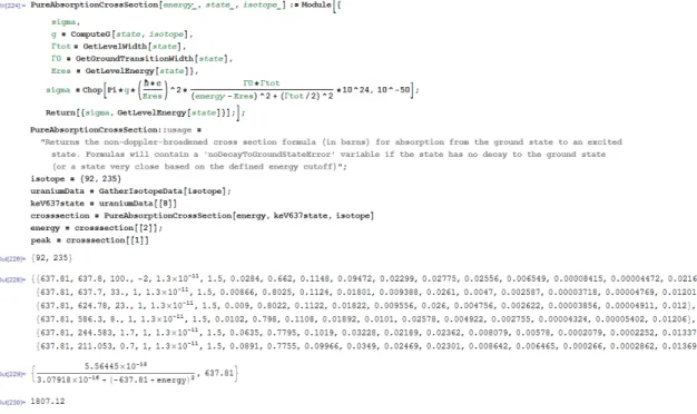
Because of Mathematica’s methods for managing functions and variables, unde-fined variables can be given to functions. This allows for on-the-fly definitions of more complex functions, such as the NRF cross section of an excited state in terms of energy. The definition of the PureAbsorptionCrossSection function which computes Equation 2.4, the cross section for excitation of an isotope from the ground state to a given excited state, is found in Figure 3-4. The function calculates the cross section and returns it as the first element in a list. The second element of the list is the resonance energy, which is helpful for subsequent reference and plotting.

Additional functions have been defined for other cross section computations, such as for individual decay modes, energy-integrated values, and for Doppler-broadened calculations. These functions have been omitted here for brevity, but some are utilized below.

3.1.2.2 Plotting

The notebook also contains several extensions of Mathematica’s built-in plotting ca-pabilities to quickly visualize the NRF properties of an isotope of interest. The

Figure 3-4: Definition and usage of the PureAbsorptionCrossSection function. The function implements Equation 2.4. Here it is used to derive the formula for the cross section of a U235 resonance and to solve for the peak height in barns.

function BuildPlots has been implemented to take a list of energy-dependent cross section equations along with a list of plotting options and return an array of plots that can then be overlaid into a single output. An example of its use is found in Figure 3-5

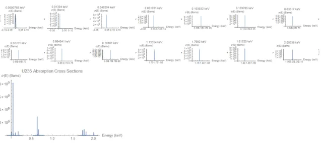
Likewise, the PlotIntegratedCrossSections function creates an easy-to-read plot of energy-integrated NRF cross sections for a given isotope, allowing users to quickly compare resonance strengths.

3.2 Bayesian Inference of Foil Properties

3.2.1 Objectives

3.2.1.1 Modeling Uncertainty and Knowledge Gain

The primary goal of the second part of this thesis is to simulate the methods an inspector might use to estimate properties of the foil and warhead and to test their

Figure 3-5: Usage of the BuildPlots function. The function implements plotting of energy-dependent cross sections. Note that because the resonances are so narrow yet span such a wide range in energies, Mathematica may clip or exclude lines if the plotting resolution and recursiveness are not set high enough.

Figure 3-6: Usage of the PlotIntegratedCrossSections function. The function imple-ments simplified plotting of energy-integrated cross sections. If the PlotRange -> All option is omitted, the function defaults to plotting cross sections with the same axes limits.

effectiveness. One such mechanism of inference is a Bayesian update algorithm. In this case, such an algorithm starts with a uniform or otherwise guessed initial prob-ability distribution for the span of possible material properties. Then, each possible combination of foil and warhead material properties (at each branched or neighboring pair of NRF peaks) can be analyzed for its likelihood given the measured information

and used to update the probability distribution. A successful inference process results in a probability distribution that confidently predicts the actual properties of the test object or foil. Therefore, one objective of this investigation is to implement this pro-cess and determine both the challenges and outcomes an inspector might realize by implementing such an algorithm.

3.2.1.2 Verification of Theoretical Model of Inference

Secondly, this work attempts to validate the theoretical model of knowledge gain being developed by Ruaridh Macdonald and discussed in Section 2.2.3. Macdonald’s developments constitute a valuable understanding of inference and knowledge gain processes in a warhead verification scenario, and these simulations and results hope to substantiate some of the useful formulations that he has developed.

3.2.2 Implementation

3.2.2.1 High Level Organization

In terms of organization, the code is divided into two separate parts. Firstly, the code imports data from a .csv file created by the Mathematica notebook discussed in Section 3.1. This file contains not only NRF data, but also data on the non-resonant attenuation properties of each material of interest from the XCOM database [21]. At this point, the code also uses this data to create an NRFGamma class object to simulate the actual one-dimensional behavior of photons at each resonance energy, resulting in a final number of counts detected. Secondly, the code performs a Bayesian analysis of these resonances and simulated count information to inform an updated probability distribution of inferred foil properties. Like the Mathematica notebook, the full Python 2.7 codebase used to implement the inference model is available in the Appendix. Ruaridh Macdonald was instrumental in creating this program and contributed immensely to the code, which also utilizes code developed by Jayson Vavrek.

3.2.2.2 Data Processing and Initial Conditions

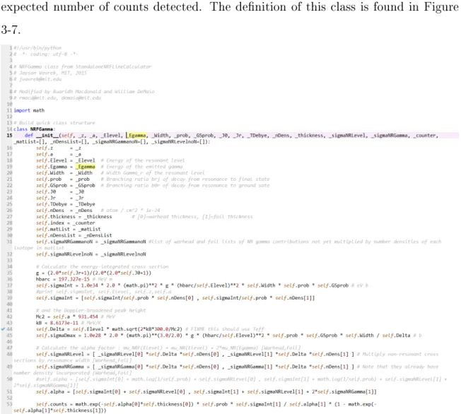
Initially, the code takes in command-line arguments for variables such as the energy range of interest and location of the matList file loaded with material properties for the simulation. After performing checks on the inputs, the load_line_data function processes the data and input files to create a Python list of emission lines referred to as emitList. Each entry in emitList is an NRFGamma object. During the initial declaration of these objects, calculations are performed by the code to simulate the expected number of counts detected. The definition of this class is found in Figure 3-7.

Figure 3-7: Definition of the NRFGamma class originally developed by Jayson Vavrek. This version has been extended to implement the Bayesian update algorithm.

After performing some cleanup, such as removing emissions weaker than a user-defined count threshold from emitList, this list of NRF line data is given as a

param-eter to the NRFmultiLine.branchNeigh_compare function. This function processes the emission data and, based on the passes parameters, returns lists of branched and neighboring NRF peak pairs.

3.2.2.3 Bayesian Update Algorithm

Once the branched and neighboring pairs to be analyzed have been identified, the code populates several lists with guessed foil parameters and uniform probability dis-tributions. Consistent construction and ordering is retained throughout this process, so that the code can later loop through each list when performing calculations. As discussed in Section 2.2.3, the key variables of interest are the foil thickness, war-head thickness, and the number densities of the isotopes in both the foil and the warhead. These number densities correspond to 𝛼1 and 𝛼2 values at a resonance energy according to Equation 2.23, meaning that a given 𝛼 value can be determined by a large number of possible combinations of areal densities if there are multiple isotopes present. Therefore, these 𝛼 values need to be calculated for each individual pair under consideration, and each corresponding result must update the probability distribution of its component number density values.

Figure 3-8 shows the organization of the probsFoilHistory list, which stores the probability distribution of foil thickness guesses as the algorithm proceeds through each peak pair. Initially, the user enters bounds and a ∆ value, which populates the first row of this list. From there, the code proceeds downwards and updates the expected probabilities of each thickness value being correct for each pair, given the previous probability distribution. The corresponding values are stored in the valsFoil list. Similar arrays are constructed for warhead thickness and number density probability distributions.

Using this construction, the code must perform Bayesian updates for every com-bination of number densities and thickness values in the warhead and foil. During the branched pair inference process, for example, the algorithm runs the update code shown in Figure 3-9.

⎡ ⎢ ⎢ ⎢ ⎣ [︀𝑝𝑡11 𝑝𝑡12 𝑝𝑡13 . . . 𝑝𝑡1𝑛 ]︀ [︀𝑝𝑡21 𝑝𝑡22 𝑝𝑡23 . . . 𝑝𝑡2𝑛 ]︀ ... [︀𝑝𝑡𝑚1 𝑝𝑡𝑚2 𝑝𝑡𝑚3 . . . 𝑝𝑡𝑚𝑛 ]︀ ⎤ ⎥ ⎥ ⎥ ⎦

Figure 3-8: Organization of the probsFoilHistory matrix. Each value column tracks the probability of one guess of a foil thickness value, and each row corresponds to a pair being analyzed.

Figure 3-9: Implementation of the Bayesian update algorithm. 3.2.2.4 Challenges

Due to the multidimensional nature of the problem at hand, runtimes and data usage can grow quickly. Increasing the resolution of the simulation has strong exponential effects, and consideration of more than a few isotopes will also greatly inflate the scope of the simulation.

Additionally, data sources and accuracy can have large effects on results. Incom-plete resonance data or poorly interpolated non-resonant attenuation estimates will greatly reduce the amount of information it is possible to obtain during the infer-ence process. A program of this sort is also subject to many potential problems, such as errant variables causing large sways in probability distributions or producing nonphysical results.

3.2.2.5 Solutions

Managing these difficulties is possible, but can be a time consuming process. Intelli-gently limiting intermediate calculations performed in each loop can help to manage

the runtime problem, and through smart organization, forethought, and trial and er-ror, the inference process can be made suitably efficient. Most of the tests performed in the next section take on the order of 10 − 10, 000 seconds to complete and used up to 1 GB of memory. However, some statistical simplifications were made to achieve these low runtimes. Chiefly, mean values of measured counts are used rather than stochastic algorithms. Uncertainty is instead modeled by the spread of the resulting probability density function given by assuming a Gaussian distribution centered on the correct answer. The computing time goes roughly as the number of guesses to the power of the number of isotopes. Therefore, simplified test cases must be utilized in order to obtain useful results in a timely manner. Simulations with more than four isotopes with small ∆ values were not attempted.

In order to suitably manage the data utilized by the algorithm, continuous double-checking of resonances, variables, and results is necessary. For example, by inspecting probability distribution shifts over time, it is possible to identify NRF peaks with bad or incorrectly processed data that would otherwise disproportionately sway results. The Mathematica notebook has proven extremely useful for visually verifying data, analyzing specific peaks, and identifying problems.

Results

4.1 Testing

Before the inference algorithm can be used to draw conclusions about real-world verification scenarios, validation tests must first be performed to ensure the code is functioning properly. Below, the inputs and outcomes of several testing cases are discussed.

4.1.1 Overall Performance

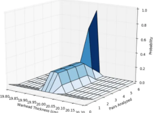
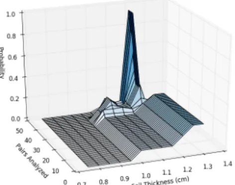
In most cases, the algorithm was able to successfully predict foil and warhead prop-erties as long as the input parameters allowed for suitable information gain. Figures 4-1 and 4-2 visualize the inference process for the foil and warhead thicknesses. The surfaces plotted display the probabilities that each value is the correct one. As is shown, each successive peak pair analyzed updates the previous probability distri-bution, usually towards a more refined guess. Flat regions of the probability surface usually indicate that the solution has converged, or that some peak pairs were skipped because they did not meet the minimal number of counts. Figure 4-3 shows the correct determination of number densities of four isotopes in a test scenario.

Non-convergence can be caused by several factors. When the selection of guesses does not contain the actual values, the solution rails to one side or does not converge, as shown in Figure 4-4. This is an ideal behavior, as it indicates that a solution could not be found. Rarely, floating point errors, roundoff errors, or other behaviors can prevent the formation of an accurate solution when one is possible. Performing

(a) A foil thickness probability surface.

Ac-tual thickness: 1 cm. (b) A warhead thickness probability surface.Actual thickness: 20 cm. Figure 4-1: Development of thickness estimates with successive peak pairs. Initially, a uniform likelihood is assumed for each potential value being analyzed. Then, the algorithm iteratively updates these guesses by calculating the probability of observing the actual ratio of counts at each branched or neighboring NRF peak pair if these values were the true values. While these visualizations are not quite rigorously-defined probabilistic surfaces, they are convenient mechanism for comparing the likelihood of specific inferred values being correct, as well as for tracking changes in the inferred probability distribution throughout the simulation.

(a) A late-converging foil thickness

probabil-ity surface. (b) A warhead thickness probability surfacedisplaying modal behavior. Figure 4-2: Convergence of probability distributions. For some sets of input param-eters, there is a chance that an accurate probability distribution will not be found, or will be slow to converge. Figure 4-2b shows another behavior, the development of alternate stable modes in the solution. These modes likely correspond to other combinations of thickness and number density guesses which produce 𝛼 ratios similar to those observed.

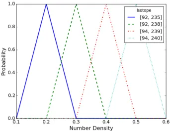
Figure 4-3: Determination of number densities for multiple isotopes. Here, the algo-rithm converged to the correct number densities assigned to each of the four isotopes (in 1024_{𝑎𝑡𝑜𝑚𝑠/𝑐𝑚}2_).

additional simulations with slightly varied parameters usually resolves these problems.

Figure 4-4: Example of a non-convergent solution when the actual value is out of range. In this case, the real number density of U235 is above the limits of the guessing interval.

One feature of Bayesian inference is the potential to use a non-uniform prior, that is, a modified selection of initial guess probabilities potentially influenced by an inspector’s previous knowledge. Even if the initial guesses do contain the correct value, an incorrect prior may still prevent the algorithm from converging on the correct posterior distribution. Figures 5a and 5b show these problems. Figure 4-6a displays an initial probability distribution which does eventually result in a correct

solution, and Figure 4-6b shows the control case.

(a) A non-converging prior which did not

con-tain the true value of 1 cm. (b) A non-converging prior which did containthe true value of 1 cm. Figure 4-5: Two non-convergent Bayesian priors. The figure on the left does not contain the correct value, and therefore could never converge, while the figure on the right was simply unable to find the correct solution.

(a) A converging non-uniform prior which did

contain the true value of 1 cm. (b) Control case with a uniform initial prob-ability distribution. Figure 4-6: Figure 4-6a displays a non-uniform initial probability distribution that successfully converges. Figure 4-6b shows the control case for these three tests where a uniform initial probability distribution was used. All other inference simulations performed here utilize uniform priors.

4.1.2 Effects of Initial Conditions and Variables

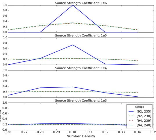
One of the primary variables of interest is the gamma source strength. In a verification scenario, more powerful photon sources, as well as longer counting times, may greatly increase the leakage of information to the inspector. Therefore, the effect of source strength on the inference process was examined while all other parameters were held constant (see Table 4.1). The results for the case of four isotopes with equal number densities are displayed in Figures 4-7 through 4-9. Here, the source strength coefficient refers to the minimum number of detected counts at the strongest resonance for every isotope. In other words, each isotope under consideration must have at least one peak with a minimum number of counts equal to the source strength coefficient.

Material U235 U238 Pu239 Pu240

Foil Number Density (1024_{𝑎𝑡𝑜𝑚𝑠 /𝑐𝑚}2_{) 0.30 0.30 0.30 0.30} Warhead Number Density (1024_{𝑎𝑡𝑜𝑚𝑠 /𝑐𝑚}2) 0.30 0.30 0.30 0.30

Foil Thickness (cm) 1.0 1.0 1.0 1.0

Warhead Thickness (cm) 2.0 2.0 2.0 2.0

Table 4.1: Material parameters for source strength testing.

Indeed, stronger source terms allowed for much more certainty when predicting foil and warhead properties. In this specific case, several strong neighboring peaks in uranium 235 resulted in much higher numbers of counts for this isotope, greatly increasing information gain. Only in the cases with the highest source terms would an inspector be able to make good predictions about the number densities of the other isotopes present.

However, all cases produced some information about the foil and warhead thick-nesses, though certainty did decline for smaller source terms. Because branched peaks only contain usable information about the foil, and dozens of branched peaks were able to be analyzed for each source strength case, all of the foil thickness probability distributions (Figure 4-8) were relatively refined. However, only in the cases of very strong source terms was much information leaked about the warhead. A large factor

Figure 4-7: Effect of the source strength parameter on number density inference in the foil. In these cases, all isotopes had an actual number density of 0.30·1024_{𝑎𝑡𝑜𝑚𝑠/𝑐𝑚}2_. Predictably, stronger sources (or longer counting times) may allow an investigator to predict foil properties with greater certainty. Notably, U235 has several strong, neigh-boring resonances in the middle of the energy range analyzed, leaking significantly more information in this case. For these tests, little information was directly leaked about the warhead composition (not shown).

in this outcome was likely the exclusion of some of the weaker neighboring peaks due to low count numbers. With a source parameter of 106, six neighboring peak pairs had strong enough signals to be analyzed according to the prescribed minimum cut-off parameter. In the case of the weakest source term, only one such pair was consid-ered. A summary plot showing the relationship between correct inference results and source strength can be found in Figure 4-10. The most statistically significant iso-tope, U235, displays a roughly logarithmic improvement in inference with increasing

Figure 4-8: Effect of the source strength parameter on inference of the foil thickness. Here, foil thickness was held constant at 1 cm.

Figure 4-9: Effect of the source strength parameter on inference of the warhead thickness. In these cases, the warhead thickness was held constant at 2 cm.

source strength.

4.1.2.2 Gaussian Delta Value

During the Bayesian update process, a ∆ value must be used to convert the continuous probability of the assumed Gaussian distributions of the variables to the discretized form of the probability distributions being calculated. In this case, ∆ is one half of the spread used for taking the area of the cumulative distribution function when calculating the probability of a guessed value being correct. Larger ∆ choices should have a smoothing effect, especially as ∆ becomes greater than the interval between guesses. This is because each guess has a higher chance of encompassing the real value

Figure 4-10: Summary plot displaying inference outcomes by source strength coeffi-cient. The vertical axis displays the height of the posterior probability distribution for each isotope at the correct number density value in the foil. U235, which leaked the most information, displays a roughly logarithmic improvement with increasing source strength.

Material U235 U238

Foil Number Density (1024_{𝑎𝑡𝑜𝑚𝑠 /𝑐𝑚}2_{) 0.30 0.30} Warhead Number Density (1024_{𝑎𝑡𝑜𝑚𝑠 /𝑐𝑚}2) 0.30 0.30

Foil Thickness (cm) 1.0 1.0

Warhead Thickness (cm) 20 20

Table 4.2: Material parameters for Gaussian ∆ testing.

for the purposes of the calculations. Conversely, narrower ∆ values should have the opposite effect, allowing for faster convergence, but increasing the chances that the real value is missed entirely. Figure 4-11 shows the difference in convergence as peak pairs are analyzed using relatively high and low ∆ values. The material properties used for these simulations are listed in Table 4.2.

For the test cases run, ∆ values higher than 10 did not allow the distribution to converge, while values lower than 0.001 caused the solution to destabilize before all of the pairs had been processed. Figure 4-12 displays the varying levels of information obtained about the foil in some of these cases.

(a) Convergence of foil thickness probability

distribution for Δ = 1. (b) Convergence of foil thickness probabilitydistribution for Δ = 0.001. Figure 4-11: Comparison of convergence with high and low ∆ parameters. In this set of tests, higher ∆ values led to slower convergence. For a ∆ of 1.0 on the left, departure from the uniform distribution was not achieved until pairs with very high 𝛼 ratios (∼ 4) were processed.

a thickness of 20 cm and number densities of 0.3 · 1024_{𝑎𝑡𝑜𝑚𝑠/𝑐𝑚}2 _{for both isotopes} included. This result can be seen in Figure 4-13.

Figure 4-13: Posterior distribution from inference of warhead composition with ∆ = 0.001. This was the only of the five cases which leaked any information about the warhead composition.

These tests, as well as others performed but not recorded here, show that tuning of the ∆ parameter can be a tricky process. Too big, and the solution may not converge or will reveal little information. Too small, and the solution may destabilize. Unfortunately, this sweet spot is dependent on the other input parameters. Therefore, either an array of ∆ values will need to be used for more unknown scenarios, or methods need to be developed to calculate an ideal value based on given inputs. 4.1.2.3 Guess Intervals and Foil Thickness

In order for an inspector to determine the properties of either the warhead or foil through such an inference algorithm, the correct material properties must be con-tained within the range of values investigated. However, foils that have either very high or very low 𝑋 · 𝛼 values (∝ 𝑡ℎ𝑖𝑐𝑘𝑛𝑒𝑠𝑠 · 𝑛𝑢𝑚𝑏𝑒𝑟 𝑑𝑒𝑛𝑠𝑖𝑡𝑦) could result in increased inference error [16]. These edge cases may have the potential to incorrectly sway results if included in the scope of guessed values. Figure 4-14 shows the relationship between measured results on the vertical axis and guessed values on the horizontal axis. As the slope of the curve decreases, small inaccuracies in the measured values can introduce large differences in inferred 𝑋 · 𝛼 parameters. However, since

stochas-tic measurements were not implemented, the error introduced by varying 𝑋 · 𝛼 was negligible in test cases.

Figure 4-14: Relationship of measured results to 𝑋 · 𝛼 guesses in the encrypting foil. As the curve becomes flatter, small variations in measurements may cause large changes in inferred values for the thickness and number density of the foil.

To test the effects of widening the guess interval on the estimation of number den-sity, a series of inference tests were performed over the same number of intervals, but with a varying interval width. The material parameters for these investigations are displayed in Table 4.3. Overall, results indicated that satisfactory inference remains

Material U235 Pu239

Foil Number Density (1024_{𝑎𝑡𝑜𝑚𝑠 /𝑐𝑚}2_{) 0.34 0.36} Warhead Number Density (1024_{𝑎𝑡𝑜𝑚𝑠 /𝑐𝑚}2_{) 0.30 0.30}

Foil Thickness (cm) 1.5 1.5

Warhead Thickness (cm) 20 20

Table 4.3: Material parameters for guess interval testing.

possible even with large spans of number density guesses. Convergence onto guesses close to the defined values occurred in almost all cases. Below, Figures 4-15 and 4-16 give the inference results in the narrowest and widest cases, respectively.

Overall, wide guessing intervals only subjected the inference process to small er-rors. In order to refine their estimates, an inspector could first run the algorithm on a wide range of values, then use the results to narrow subsequent investigations.

(a) Final foil number density probability dis-tributions for a case with number density in-terval 𝑑 = 0.005 · 1024_{𝑎𝑡𝑜𝑚𝑠/𝑐𝑚}2_.

(b) Convergence of foil thickness probability distribution for a case with number density interval 𝑑 = 0.005 · 1024_{𝑎𝑡𝑜𝑚𝑠/𝑐𝑚}2_.

Figure 4-15: Probability distributions for a narrow interval case. The actual foil thickness was 1.5 𝑐𝑚, and the number densities of U235 and Pu239 were 0.34 and 0.36 · 1024_{𝑎𝑡𝑜𝑚𝑠/𝑐𝑚}2_{, respectively.}

(a) Final foil number density probability dis-tributions for a case with number density in-terval 𝑑 = 0.05 · 1024_{𝑎𝑡𝑜𝑚𝑠/𝑐𝑚}2_.

(b) Convergence of foil thickness probability distribution for a case with number density interval 𝑑 = 0.05 · 1024_{𝑎𝑡𝑜𝑚𝑠/𝑐𝑚}2_.

Figure 4-16: Probability distributions for a wide interval case. The actual foil thickness was 1.5 𝑐𝑚, and the number densities of U235 and Pu239 were 0.34 and 0.36 · 1024𝑎𝑡𝑜𝑚𝑠/𝑐𝑚2, respectively. Here, with the widest number density interval tested, only slight errors are observed, most notably the low estimate of foil thick-ness. Equivalent results were obtained with more detailed foil thickness distributions as well as with a thinner foil.

4.1.2.4 Isotopic Considerations

Because all isotopes have unique nuclear resonance properties, their effects on infer-ence processes are similarly varied. Though only a handful of isotopes have been

investigated here, their ubiquity in nuclear weapons makes understanding their inter-actions critically important for the development of a nuclear warhead disarmament treaty. For example, U235 has numerous strong resonance peaks in the 0.5-10 MeV range, which tended to dominate information leakage in many of the cases analyzed. One notable peak is the 637.81 keV resonance, which has several branches with 𝛼 ratios up to 1:5.6 (when it decays via emission of a 211 keV gamma). In a testing scenario, a low energy filter may need to be introduced in order to negate the infor-mation leakage potential of this and similar decay modes. In the Python code, these peaks can be excluded by raising the minimum detector energy parameter. Figure 4-17 shows the peaks typically analyzed for four isotopes. In general, 𝛼 ratios farther from 1 leak more information, and higher numbers of counts increase the certainty of this information.

(a) Selection of peak pairs analyzed in a

typ-ical branched pair inference simulation. (b) Selection of peak pairs analyzed in a typ-ical neighboring pair inference simulation. Figure 4-17: Peak pairs analyzed in a typical inference simulation. As shown in both figures, U235 tends to dominate the inference process if it is present, as it provides an assortment of strong peak pairs with varied 𝛼 ratios. It is also the only isotope with neighboring pairs which satisfy the set minimum requirements of this specific simulation. U238 has too few peak counts to be shown on either plot, and the plutonium isotopes provide only a few branched pairs of use.

Uranium 235’s prominent peaks do not mean that other isotopes have no utility for inference. If U235 is excluded from the investigation, other isotopes may still contribute significant amounts of information, such as in the case of two plutonium isotopes investigated in Figure 4-18. However, the counting times necessary to achieve

similar levels of certainty will necessarily be much higher for tests conducted without consideration of U235. Additionally, the lack of neighboring pairs (within 10 keV) from the other three isotopes studied makes the inference of warhead properties much more difficult, as ignoring the variation of the bremsstrahlung spectrum to include more distant pairs will introduce increasingly significant errors.

Figure 4-19 shows the plutonium case with the addition of U238. This inclusion increases the certainty of the number densities inferred, but this effect is largely due to the substantial increase in counts required to get the strongest U238 peak above the minimum count threshold for the test. As discussed in Section 4.1.2.1, the source strength criterion used requires that the tallest peak of each isotope under consideration meet a certain minimum number of counts. In under these conditions, the strongest U238 resonance included for analysis, the 2.754 MeV resonance, was 17 orders of magnitude weaker than the plutonium resonances. Therefore, inclusion of U238 into the minimum count criterion results in astonishingly large counting times and/or source strengths, and greatly increases information leakage.

(a) Number density inference of Pu239. (b) Number density inference results for Pu239 and Pu240

Figure 4-18: Inference simulation of number density with two plutonium isotopes. For both isotopes, the actual number density was 0.30 · 1024_{𝑎𝑡𝑜𝑚𝑠/𝑐𝑚}2_{. In this case,} information about the foil is leaked only through the branched peak pairs of these two isotopes, albeit at a much lower rate than is possible with U235.

Figure 4-19: Inference of number density with Pu239, Pu240, and U238. The strongest U238 resonance included for analysis based on the input data was 17 or-ders of magnitude weaker than some of the plutonium resonances. Inclusion of U238 into the minimum count criterion would result in staggeringly large counting times or source strengths, and would also greatly increase the certainty of leaked information.

4.2 Scenario Analysis

4.2.1 Testing Parameters and the Black Sea Warhead

After validating and characterizing the behavior of the inference code, a trial scenario was analyzed. Using reconstructed data in the public domain about a Soviet warhead design, a one-dimensional simulation was constructed and evaluated [22]. In this case, the warhead and foil were assigned the properties shown in Table 4.4. Due to memory limitations, as well as its effects on source strength, U238 was left out from this analysis.

4.2.2 Properties Inferred

Four foil thicknesses: 1,2,3, and 4 cm were tested for their ability to resist inference. The resulting number density probability distributions are displayed in Figure 4-20. Overall, outcomes for warhead property inference were similar in each case, with all four foils revealing considerable information about the thickness of the warhead, but