A coning motion apparatus for hydrodynamic model testing in a non-planar cross-flow

(1)

A CONING MOTION APPARATUS FOR HYDRODYNAMIC MODEL TESTING IN A NON-PLANAR CROSS-FLOW

by

DAVID CRAIG JOHNSON B.S., Aerospace Engineering United States Naval Academy

(1982)

Submitted to the Departments of Ocean Engineering

and Mechanical Engineering in Partial Fulfillment of the Requirements for the Degrees of

NAVAL ENGINEER and

MASTER OF SCIENCE IN MECHANICAL ENGINEERING at the

MASSACHUSETTS INSTITUTE OF TECHNOLOGY

June 1989

@ Massachusetts Institute of Technology 1989

Signature of Author

-Departments of Ocean Engineering and Mechanical Engineering June 1989 Certified by

Justin E. Kerwin, Thesis Supervisor Professor of Ocean Engineering Certified by

Harri K. Kytimaa, Thesis Reader Assistant Professor of Mechanical Engineering

Accepted by , _{A. Douglas Carmichael, Chairman}

Departmental Graduate Committee Department of Ocean Engineering Accepted by ..- .

Ain A. Sonin, Chairman Departmental Graduate Committee Department of Mechanical Engineering

A CONING MOTION APPARATUS FOR HYDRODYNAMIC MODEL

TESTING IN A NON-PLANAR CROSS-FLOW

LT David C. Johnson

Department of Ocean Engineering, MIT

Submitted to the Departments of Ocean Engineering and Mechanical Engineering on 12 May 1989 in partial fulfillment of the requirements for the

Degrees of Naval Engineer and Master of Science in Mechanical Engineering

Abstract

As part of continuing research into the flow about slender bodies of revolution, a con-ing motion apparatus for hydrodynamic model testcon-ing was built and demonstrated. This is the first known use of a rotary balance apparatus for extemal flow hydrodynamic

applications. The rotary rig allows for captive model testing with simultaneous roll and yaw components, and with non-planar cross-flow effects. Coning characterizes the non-planar nature of a general motion that cannot be constructed from contributions due to any planar motions.

Demonstration tests were conducted with a length/diameter = 9.5, body of revolution. Force and moment measurements were taken via an internally mounted, 6-component bal-ance, capable of capturing all six force and moment components acting on the model. The tests covered coning angles to 20', spin rates to 200 rpm, and free stream velocities to 30 ft/s. Reynolds number based on model length ranged from 4.04x106 to 6.06x106. Cross-flow Reynolds number based on body diameter extended from 1.5x105 _{to 3.0x10', covering flow} regimes near the transition from laminar to turbulent separation. The non-dimensional forces and moments generally show a non-linear variation with spin rate for coning angles greater than 14'. The measured out-of-plane force was significant, reaching a magnitude of 30% of the in-plane force. Experiment data correlated fairly well with numerical predictions (using laminar separation criteria).

Thesis Supervisor: Dr. J. E. Kerwin, Professor of Ocean Engineering

(3)

Acknowledgements

The successful completion of this project would never have been possible without the considerable effort of several individuals. From the start, the experiment required team par-ticipation from all the players: General Dynamics, Electric Boat Division and Convair Divi-sion, Stevens Institute of Technology, Davidson Laboratories, MIT and Nielsen Engineering and Research. I would like to give special thanks to the following individuals:

- Dr. Chuck Henry and Gerry Fridsma of Electric Boat, for their sponsorship of the

study, their technical guidance and encouragement, and their origination of the coning motion concept for external flow, slender body of revolution experiments.

* Dr. Peter Brown, Dr. Glenn Mckee, Dick Krukowski, and the model shop personnel of Davidson Laboratories for their great effort in not only building the model and apparatus, but assisting in getting it to work.

* Phil Mole and the calibration team at Convair for their excellent work in preparing the balance for use.

* Mike Mendenhall and Stanley Perkins of NEAR for their SUBFLO numeric studies that were invaluable for data comparison.

* Dr. Jake Kerwin and Dr. Harri Kyt6maa of MIT for their active involvement with the study and their help.

* LT Norbert Doerry, a fellow MIT 13A, for his assistance in many aspects of the proj-ect.

* A very special thanks to S. Dean Lewis of the MIT variable pressure water tunnel, who designed all of the mechanical components for the tunnel modifications and assisted with their installation. His help was invaluable!

* Ronnie St. Jean and the Nuclear Engineering Machine shop for their instant service in building and modifying the many components for the test.

* Finally, a very special thanks to my wife, Carol, who patiently stood by through all the trials of getting a new experiment up and running, and provided the moral encouragement to complete this project.

(4)

Chapter 3 Test Procedure and Tare Measurements ... 35

3.1 Balance Calibration and Check-out ... ... 35

3.1.1 Data Reduction Model ... ... .. 36

3.1.2 Balance Operation ... ... ... 37

3.1.2.1 Weight Calibration and Axis Convention ... 38

3.1.2.2 Model Weight and CG ... .... ... 39

3.1.2.3 Temperature Effects ... ... 40 3.2 T est Procedure ... ... 41 3.2.1 T est L ogic ... 41 3.2.2 Code Development ... 43 3.2.2.1 T im ing ... 43 3.2.2.2 Desired Results ... ... 45 3.3 Tare Measurements ... 47 3.3. 1 S tatic ... ... 4 8 3.3.2 R otational ... ... 48 3.4 T est M atrix ... 53

Chapter 4 Test Results ...

54 Chapter

5 Data Analysis ...

64

5.1 Comparison with Numerical Results ... ... 64

(5)

Chapter 6 Conclusions and Recommendations ...

77 6.1 C onclusions ...

77 6.2 Recom m endations ... ... 78

REFERENCES ...

80 Appendix A Taylor Series Expansion ... 82

Appendix B Inertia, Gravity and Buoyancy Forces ...

90 Appendix C Test Data ...

96 Appendix D FORTRAN Routines ...

111

(6)

Table of Figures

Coning Motion ... 11

Flow types and force regimes for increasing angle of attack ... 14

Unappended body of revolution cross-flow ... 15

L/D=9.5 hull in coning motion ... 16

Mathematical model process ... 18

Coning m otion m odel ... 20

Coning motion model and balance assembly ... ... 21

Coning m otion apparatus ... 23

Torsional vibration m odel ... ... ... ... ... 27

Forces measured by balance for constant rotation rate ... ... 30

Coning motion apparatus in tunnel test section ... ... 31

Data acquisiton and reduction system ... ... 32

Phase shift in raw count data ... 45

Phase shift vs frequency ... 46

Amplitude ratio vs frequency ... ... 47

X and Z Inertia Forces, 20' ... 50

M Inerial M om ent, 20' ... ... 50

X and Z Inertia Forces, 14' ... 51

M Inertial M om ent, 14' ... ... 51

Y' and Z' non-dimensional forces, 20' ... ... 55

M' and N' non-dimensional moments, 20' ... ... 56

M' and N' non-dimensional moments, 14' ... ... 58

M' and N' non-dimensional moments, 8' ... ... 60

Y ' vs coning angle ... 61

N ' vs coning angle ... ... 62

Predicted and experiment non-dimensional forces ... 67

Predicted and experiment non-dimensional moments ... 68

Summed raw counts output, 20", 30 ft/s ... ... 69

FFT of N1 & N2 raw counts, 200 rpm ... ... 71

FFT of N1 & N2 raw counts, inertia run ... ... 72

FFT of Y1 & Y2 raw counts, 200 rpm ... ... 73

200 RPM, Inertia and full-up run FFT results ... ... 74

(7)

LIST OF NOMENCLA TURE

Body Fixed

Axis System

x,u,p

X,K

Z,w,r

Z,N

AXES Body Fixed:

*X the longitudinal axis, directed from the after to the forward end of the model

the transverse axis, directed to starboard the normal axis, directed from top to bottom

-y

*Z

(8)

Tunnel Fixed: " XO * yo * zo * XB, YB, ZG * XG, YG- ZG * X, Y, Z *K, M, N *W *B

* _{Ix, ly, Iqz}

* m

*CB *CG

the fixed longitudinal axis, colinear with the tunnel longitudi-nal centerline.

the fixed transverse axis, perpendicular to x, in a horizontal plane, directed to starboard

the vertical axis, directed downwards COORDINATES AND DISTANCES

coordinates of the CB relative to body axes cooidinates of the CG relative to body axes

coning angle, measured from the xo axis to the x axis FORCES AND MOMENTS

force components relative to body axes, referred to as longi-tudinal, side, and normal forces respectively

moment components relative to body axes, referred to as rol-ling, pitching, and yawing moments, respectively, referenced

to the COR

weight of the model; W = mg model buoyancy force

INERTIA CHARACTERISTICS

moments of inertia of the model about the x, y, and z axes, respectively

mass of model

SPECIFIC POINTS ON BODY center of buoyancy of model center of mass of the model

(9)

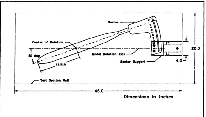
* COR Center of rotation, the reference point for all measured and calculated forces and moments, located 11.31 inches aft of the model bow, on the longitudinal axis

* BMC Balance moment center, .895 inches aft of the COR, on the model longitudinal axis

VELOCITIES

* u, v, w components along body axes of velocity of origin of body axes relative to fluid

* p, q, r angular velocity components relative to body axes x, y, z; angular velocities of roll, pitch, and yaw

* (0 _{model rotation vector in tunnel fixed axes; to = oUA,}

MISCELLANEOUS

* A model maximum cross sectional area; area projected onto y-z plane

* p density of fresh water = 1.9348 slugs/ft3(t=77'F)

(10)

A CONING MOTION APPARATUS FOR HYDRODYNAMIC MODEL TESTING IN A NON-PLANAR CROSS-FLOW

Chapter 1 Introduction

For many years, the primary goal of researchers in the motion dynamics field has been to develop the ability to accurately predict the full-scale motions of vehicles. Even today, with the powerful computational tools available, reliable motion predictions of vehicles in all portions of the maneuvering envelope are not possible. Murray Tobak and Lewis B. Shiff pointed out that the difficult problem is to correctly describe the relationship between the aerodynamic reactions and the motion variables in the inertial equations of motion of an air-craft [1]. This same difficulty applies to the motion of hydrodynamic vehicles as well. For slender body shapes with fin appendages, the problem is compounded by the complex wake structure formed by the maneuvering vehicle. The vorticity shed by the hull and appendages creates a wake field that interacts with the velocity distribution over the vehicle's surface. This in tum effects the surface pressure distribution and thus, when integrated over the body's surface, the total force on the hull/appendage combination. It is this interaction that prevents a closed-form analytic solution to the problem.

To further the understanding of the basic flow field about a slender body, the MIT Marine Hydrodynamics Laboratory has been conducting experimental studies on slender body of revolutiDin configurations, both with and without fin appendages. Previous research by Coney[2], Kaplan[3], Reed[4], and Shields[5], has focused on experimentally determining the nature and strength of the vortical wakes shed from a body of revolution, both with and without a single attached fin. Their test program included both force block measurements of

(11)

fin force and moment as well as laser-doppler velocimeter (LDV) measurements for produc-ing cross-flow velocity maps at different stations along the body and for determinproduc-ing vortex strengths.

As both a continuation of the above past research and a step in a new direction, the goal of this study is to construct and demonstrate a coning motion apparatus for hydrodynamic model testing. The primary purpose of this research is to determine the forces and moments on the model as a function of the coning rate. The need for the coning motion captive model test will be developed from both flow field and mathematical model considerations.

1.1 Coning Motion

Coning motion can be described as the continuous rolling motion of the vehicle longitudinal axis about the free-stream velocity vector. To generate such a motion in the water tunnel, the model is fixed to some type of support system that can be

rotated at conntant rotation sreed

V

about an axis that is parallel to Figure 1. Coning Motion

the free stream velocity vector of the tunnel. In accomplishing this, the model sees a constant attitude with respect to the free stream throughout a rotation cycle. This is a steady coning motion as shown in figure 1. The motion allows for combinations of roll (p') and yaw ( r') velocities simultaneously: p'= (cos ao)c', r'= (sin qc)o'.

Page 11

(12)

In a coning motion study, the experimenter has control over six variables: * V: free-stream velocity

* (o: body rotation rate •* ac: coning angle

* 3: sideslip angle

* 0: body roll angle

* d: perpendicular distance of the body reference point from the rotation axis For this study, only three of the available variables were used; V, o, and or,. The sideslip angle,

P. and the body roll angle, ý,

were set = 0. No sideslip simnplified the experiment apparatus and simplified the motion for this test. The roll angle is only signifi-cant for bodies with attached appendages. The reference point chosen for the experiment is the center of rotation, therefore d = 0.

The choice of the parameter d has a significant impact on the actual inflow velocity to the model. The reference point and the perpendicular distance from the rotation axis for this experiment were chosen to minimize inertial force effects, as shown later in section 2.3.4 and Appendix B. To be completely standard, the reference point should be a function of the body geometry (for comparison with other body shapes). The geometric reference point is the body center of volume, located on the body longitudinal axis, .8 inches forward of the center of rotation.

The coning motion apparatus has been in use by aeronautic researchers since 1926. For their purposes, the coning motion apparatus provided test data on aircraft maneuver-ability at high angles of incidence and on aircraft steady state spin motion and spin recov-ery. Later on, the mathematical model developed by Tobak and Schiff indicated that

(13)

coning motion is one of the fundamental character;',tic motions required for prediction of conventional, nonspinning maneuvers. A good historical account of the development of the coning motion apparatus and its employment at a number of test facilities around the world is given in Reference [6].

1.2 Model Testing

Current hydrodynamic captive model testing comprises planar motion simulations, mostly because of the facility limitations. Conventional captive model test types include:

* Straight tow tank or circulating water tunnel at a fixed angle of attack

* Straight tow tank or circulating water tunnel with an oscillator attached to the model (i.e., planar motion mechanism)

* Rotating arm

All of these tests suffer two major deficiencies:

* Cross-flow velocity vectors along the body length lie in a plane * No roll component of angular velocity (p)

The significance of these shortcomings can be seen by first looking at the non-planar cross-flow effects and then the roll component effects.

1.2.1 Non-Planar Cross-Flow Effects

A body of revolution with no attached appendages in a planar cross-flow will exhibit four basic flow types, depending on the angle of attack and Reynolds number. Shown in figure 2 are the four flows along with the normal and side force experienced

by an ogive-cylinder at varying angles of attack [7].

(14)

The cylinder sheds symmetric vortices with no resultant side force for angles of attack up to the onset angle of attack where the flow transitions to steady asymmetric vortex flow with substantial side force, and then to wake-like flow with minimal side force.

A mUCTN _NORMAL _mDE

VORTEX FREE FLOW

SYMMETRIC VORTEX FLOW STEADY ASYMMETRIC VORTEX FLOW WAKE-LIKE FLOW FOCRCE FORCE ANGLE OF ATTACK

Figure 2. Flow types and force regimes for increasing angle of attack on ogive-cylinder.

Experiments conducted at MIT by Shields[5] on a submerged body of revolution at a Reynolds number of approximately 6 x 106 based on model length and at moderate angles of attack (up to 14') demonstrated that the body shed symmetric vortices for all angles of attack. The plot of perturbation velocities for a= 14' shown in figure 3 clearly depicts the two symmetric body vortices. The symmetry here is a direct result of the planar cross-flow that the model is exposed to.

V, -- o ill

4

V.--O VORTEX FREE FLOW SYMMETRIC VORTEX FLOW STEADY ASYMMETRIC VORTEX FLOW WAKE-LUKE FLOW

(15)

Some work has been accomplished on captive models subjected to non-planar cross-flows. Visual studies done by Tobak, Schiff, and Peterson [8] on a body of revolution in coning motion clearly portrayed the asymmetric vortex field shed by the body in the non-planar cross-flow. -- * =.do# g.m * U P 0 p * P 0 0 * * 0 9 0 9 a a P771 * U F 1 * . P I * P P 9 * a * U * P -IAm -. M . @AD m g.M em .m

Figure 3. Unappended body of revolution, a = 14'.

More recently, Nielsen Engineering and Research (NEAR) has run a coning motion case with their SUBFLO, vortex cloud computer code and predicted similar results [9]. The preliminary results are shown in figure 4 for a length/diameter = 9.5 body of revolution in coning motion with o=20". The predicted out-of-plane force (i.e., side or Y force) was 50% of the normal (Z) force value.

Page 15 G.= _r--m"v-I I • - • lI , , , , , , , , , , I , ,

(16)

Current model test techniques cannot capture this effect because of their pla-nar flow limitations. Since actual sub-mersibles rarely operate in a planar cross-flow, the coning motion test provides a more realistic test condition

for obtaining coefficient data. Coning characterizes the non-planar nature of a general motion that cannot be con-structed from contributions due to any planar motions. The presence of the non-planar motion is a prerequisite for the existence of the coupling terms that are so important in accurately describing the general motion of a six degree of freedom body (e.g., yaw-pitch

cou-pling).

0 0 c 0 X x X X 0 o ₀ o 0 0 x Sx x/L= .59 9XXX x x x x x X X X X 0 0 o 0 oo o 0 0o X XX , xx

Figure 4. L/D = 9.5 hull in coning motion; c=20", p'= .82, r'= .30.

1.2.2 Roll Component Effects

The Taylor Series expansion approach that is described in section 1.3 produces many coefficients with a roll component, p'. In the past, these hydrodynamic deriv-atives have been ignored, mostly because of the inability to obtain model test data for

x X

X

(17)

these derivatives. Three pertinent examples are the linear derivatives, Y'>, K',, and N',, for which there is little or no experimental results available [10]. K',, the linear roll damping, is believed to be important on the basis of theory, and has been shown in model tests of missiles to be an even function of angle of attack and to vary considerably for angles of attack above 5' [10].

There are two classes of higher order hydrodynamic derivatives involving roll that are of importance:

* Nonlinear variations of roll damping rate with angle of attack:

e K'V'., K',,, K',,

* Nonlinearities associated with cross-flow drag:

SY'P. Z', K'I M'I N'

The nonlinear roll damping terms will have a much greater influence on an axisymmet-ric body with an attached fin than the body used in this experiment. The cross flow drag terms are associated with the nonlinear variation of the cross force with the model angle of attack.

1.3 Hydrodynamic Math Model

The forces and moments acting on a submerged vehicle are generally non-linear functions of the linear and angular displacements, velocities, and accelerations of the vehicle and the motion of the control surfaces relative to the fluid [11]. Ideally, the func-tional relationship between the forces and moments and the motion and control parameters would be known and used directly in forming the equations of motion. Unfortunately, the functional relationship is generally unknown. Without this relationship, the function is expressed as a Taylor Series expansion with respect to the rectilinear and angular velocity

(18)

components about a chosen condition. For this study, the chosen condition is straight and level operation at the instantaneous surge velocity, u(t). Appendix A details a 3" order Taylor Series expansion and simplification for representative forces and moments.

For any mathematical representation of a physical process, the validity of the mathe-matical model depends on whether the assumed form of the equations of motion ade-quately represent the physical hydrodynamics and whether the resulting coefficients are realistic. It is not the purpose to this study to validate the use of a Taylor Series expansion as a mathematical modeling tool for this case, but rather to present the framework for the use of the force and moment data obtained from experiment. The interrelation of the math-ematical model, theoretical work, and model test data is best described by figure 5. The experimenter's purpose is to provide the experimental results (e.g., non-dimensional forces

and moments) and the understanding of the dynamics involved to validate the theoretical work, thereby improving the comprehension of the actual physical processes at work.

Figure 5. Mathematical model process.

The Taylor series expansion is advantageous from the standpoint that it is numer-ically efficient and provides a convenient structure for correlating data. However, it has

(19)

the disadvantage in that truncation of the series to a certain order limits the range of applicability from the expansion point. Current motion simulators require expansions up to 4' order to adequately model yaw-pitch coupling and 5" order for slender body lift. In addition to the algebraic burden of the high-order expansion, for the formulation to be use-ful, the coefficients must be accurately determined.

A simplified expansion for the X force equation, retaining only linear terms is as shown:

X' =X'o + (X,' +X',.w' +X',p' +Xq' +X'r') +...

The typical coefficient of a linear term in the expansion takes the form of a partial derivative of a force or moment component with respect to a variable evaluated at the

orig-inal condition; for example,

X

The form of the hydrodynamic formulation is determined by the coefficients resulting from the expansion. The coefficients determine the characteristic motions that must be evalu-ated, either analytically or experimentally. Because of the inability to analytically deter-mine the coefficients, model testing, and more recently, full scale ship trials have been used for determining not only the magnitude of the coefficients, but also which coefficients are of primary importance.

(20)

Chapter 2 Description of Test Apparatus

All testing reported in this paper was performed in the MIT Marine Hydrodynamic Laboratory's variable pressure water tunnel.

2.1 Model

Figure 6. Coning Motion Model

The model used for the experiment has the following characteristics:

* Length/Diameter 9.5 * Length 23.50 inches * Diameter 2.695 inches * Weight 10.45 lbs * Buoyancy 3.23 lbs * % Parallel Midbody 39.6%

* Length Forward 4.85 inches

* Length Aft 10.25 inches

Balance Sleeve

0 2.695 0 0

U- LI=- 4.750 --

t--

3.850o La

(21)

The model shape shown in figure 6 is the standard L/D = 9.5, body of revolution used for previous studies carried out at MIT (Ref. [3], [4], & [5]), Stevens Institute of Technology, Davidson Laboratory, and Nielsen Engineering and Research (Ref. [9]). The

shell of the model consists of three anodized aluminum pieces which mate to the stainless steel sleeve. The sleeve is mounted to the shell of the balance itself. This sleeve is the only

support for the model shell and allows the balance to sense the forces and moments experienced by the model. Void spaces in the assembly were filled with grease to prevent water leakage into the model. At the aft end of the model, some clearance from the sting was allowed to provide for model deflections. This prevented "shorting out" the balance, but also allowed some water to enter the rear cavity. The inertial force contribution from this water was calculated as negligible. The next section describes the balance itself and its waterproofing.

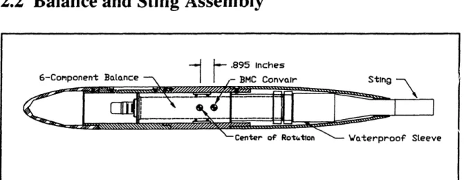
2.2 Balance and Sting Assembly

Figure 7. Coning Motion Model and Balance Assembly

Unlike past models, the present body of revolution is equipped with an internally mounted, 6-component balance for measuring hydrodynamic loads (figure 7). The balance

Page 21

(22)

provided by General Dynamics, Convair Division is a 1000 pound rated balance, calibrated to 150 lbs, and adapted for water testing. The balance was fit inside a waterproof sleeve, with the strain gage bridge wires routed out the back through a watertight seal. The bal-ance is hollow and allows for wires from the future fairwater force block to pass through the balance and out with the balance wires. Great care was taken to ensure that the fine wires coming from the balance were adequately waterproofed. Tygon tubing covered the wires from the balance to their exit out the water tunnel.

The balance consists of nine strain gage bridges: * 2 Normal force bridges

* 2 Side force bridges * 2 Roll bridges * 3 Axial bridges

Only six of the bridges are used at one time for producing force and moment readings. The preferred set of bridges was determined during the calibration done by Convair. Cali-bration of the balance is discussed in Chapter 3.

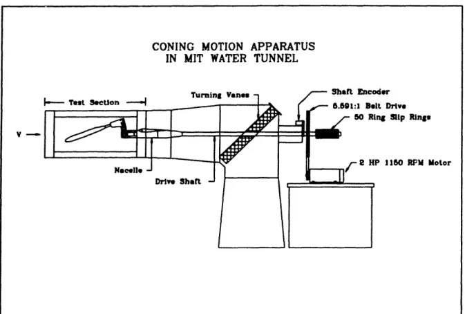
2.3 Tunnel Installation

A considerable portion of this project was spent on the design, selection, building and installation of components. During the design phase, emphasis was placed on simplic-ity, reliabilsimplic-ity, and cost. The resulting system is shown in figure 8.

(23)

CONING MOTION APPARATUS IN MIT WATER TUNNEL

- Test Section -- 4 Turning Vane

ij;u4

Nacelle

Drive Shaft

Shaft Encoder

K( - 5.591:1 Belt Drive 50 Ring Slip Rings

- HP 1180 RPM Motor

LYI I

Figure 8. Coning Motion Apparatus

2.3.1 Calculations

Because of the first time nature of this type of test in the hydrodynamics field, cal-culations of the various loads on the system had to be carried out. The calcal-culations were integral to the component selection and design process. These estimates included:

* Model drag and torque at maximum tunnel velocity and rotational speed * Model and shaft drive system speed variation at different rotational speeds

for a "free" system

* Shaft loads and system resonances * Bearing loads and wear allowances

Page 23

-ra

I ji I

(24)

r-2.3.1.1 Required Torque

The model assembly drag and torque were calculated by modelling the body as a cylinder and the sector as a flat plate. A 2-D strip theory approach was taken, where the model and sector were divided into small strips, and the drag calculated for a cross-flow velocity equal to ori for each strip with a drag coefficient based on Reynolds number:

Di = CD(P(O2 ; 2Ai)

A; is the area of each strip. Torque was then found from summing up the drag contrib-utions from each strip:

h = _i-I

X

rDii

Because of the off-center weight effect that the model and sector produced, the weight torque had to be added to the hydrodynamic torque. Weight torque was calcu-lated using the same sectioning as in the hydrodynamic case and a density of water for the model and a density of .3 lb/in3 (= p,,,,) for the sting and sector:

• ,. = (p,V,)r,

where V, is the strip volume. The resultant values for the most limiting case, a, =

20', v = 30 ft/s, co = 200 rpm, were z, = 14.9 ft-lbs, t, = 5.9 ft lbs. Finally, the mini-mum required HP was found to be:

HP .79 HP

(25)

Later testing proved two problems with this result. The first was the calculation was carried out for the preliminary sector configuration, which was more streamlined than the final design. Second, the effect of the high free stream velocity (when com-pared to the wr contribution) was neglected. The addition of the V term caused the sector to act as an inefficient foil at a varying angle of attack along its span (tunnel radius). Later attempts to model this correctly produced a very flat torque characteris-tic curve and also proved wrong. The effect of this error was the limitation of approx-imately 135 rpm for the model at 20', 200 rpm, and 30 ft/s. 200 rpm could only be achieved for the model at 20' when the free stream velocity was reduced to

approximately 10 ft/s. This problem was later fixed by placing a wing attachment on the end of the sector. The attachment was designed for a 2 to 3 degree a at 200rpm

and 30ft/s. The wing was a large success, providing enough lift to autorotate the model at 175 rpm (for V = 30 ft/s)! With the motor assisting, the model easily achieved 200 rpm.

2.3.1.2 Speed Regulation

For rotary balance experiments, it is important to maintain a constant rotation rate over a cycle of data taking. To check the worst case condition, a simple calcula-tion was done for a freely spinning system (i.e., no speed regulacalcula-tion). The model and sector were lumped together as an off-center weight of 26 pounds at a radius of gyration equal to 4.24 inches. The main sheave polar moment of inertia was calcu-lated and later obtained from the manufacturer. All other polar inertia contributions were neglected on the assumption that they were small.

For this lumped system the total J was:

(26)

J-,, (J,.d + J,•,,) = 4366in2 - lbs

The following relations were used to calculate the rpm variation:

d(Ho)

2-O - dt where H = . mIr; o , the angular momentum for this case.

dt as

Substituting: to= Xmir2d - = Jo

uil dt

Solving for the angular acceleration co:

0 = A sin(mot) where, o, = 20.9rad/s

J

Finally, the angular speed variation was found from integrating this expression:

fC

A

o= JOdt = -- cos(oot) + (o

Substituting in the numbers for 200 rpm (20.9 rad/s) and ,. = 10 ft-lbs: o = -. 507 cos(20.9t) + 20.9

This gave a worse case variation of = 4.8 rpm over 1 revolution. The advertised speed regulation for the motor would give a max variance of = 2.2 rpm over 1 cycle (1%). To avoid all of this, the main sheave was counter weighted during the inertia and data runs.

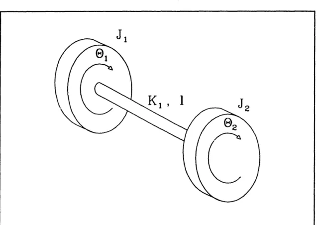
2.3.1.3 System Torsional Resonance

Unknown loads on the model-sector combination could result in a resonant vibration in the system. To investigate this, the torsional resonance frequency was

(27)

calculated for varying J's and shaft "stiffness" constants (K,). The system was mod-eled as a two disk, torsional vibratory system, shown in figure 9. The model/sector combination accounted for J,, the main sheave, J2.

Figure 9. Torsional Vibration Model

The equation for the resonant frequency was derived starting with Lagrange's equations with no forcing function:

Equation of motion: d -L = 0 , where L = T - V

dt

-1

ed

e

T'= ()J, + (• 2 (Kinetic co-energy)

V = i(j ₁ - 02) (Potential energy)

Page 27

K,,

1 J

I

(28)

Assuming an undamped system, the angles take the harmonic form:

0, =A e'"

02 = A e The resulting equation to solve is:

[ 1 O -•A, + K, K, A= 0

0

2--

dA

K -KL

Rearranging:

_-Ji2

-

KI

K,

K, - J2t02 - K [A J=[

The characteristic equation is: det[B] = 0. This leads to the desired relation for o:

[I

+J2,

ft 4

2=[- iJ2]K, ,where K,=

g

(d0 - d )

do= outer shaft diameter, d; = inner shaft diameter, I = shaft length, G = 12 x 106 psi for steel, and g = 386 in/s2. For the final system, the torsional resonance frequency -50 Hz (3000 rpm), which is much higher than the filter cutoff frequency of 3 Hz (180 rpm) and the maximum shaft rotation rate (260 rpm).

2.3.2 Modifications

The MIT variable pressure water tunnel required significant modifications before the study could be undertaken. The primary modifications necessary were:

* Boring and sleeving the turning vanes to allow for the shaft installation * Modifying the forward nacelle to accept "DU" type bushings for supporting

(29)

* Aligning and welding the bearing housing mount plate on the tunnel exterior * Installing a motor and drive system for rotating the model and shaft

Special consideration was given to the rigidity of the system since unknown reso-nances in the model-sting-drive system would have a disastrous effect on the data. The forward nacelle is rigidly mounted to the tunnel as is the exterior bearing housing assembly. The precautions proved to be worthwhile; the apparatus showed only small amplitude vibrations up to maximum system capabilities.

2.3.3 System Characteristics

The basic system characteristics are:

* Model angle of attack 0' to 20' in 2' increments * Rotations speed 0 to 200 RPM, both directions * Tunnel water velocity 0 to 30 ft/sec

* Rotary speed regulation to ± 1% for 95% change in load

* Drive motor: GE 2 HP DC shunt wound, 1200 rpm, variable speed * Drive system: 2-belt drive with drive ratios from 5.59:1 to 8.2:1 * 50 channel (rings) capability

Model rotation rate was derived for similitude in non-dimensional roll, p', with full scale vessels. Using the conventions in Appendix A, p' = 1.37 for 200 rpm at U =

30 ft/sec. The coning angle limit of 20 degrees is based on tunnel test section

dimen-sions.

(30)

2.3.4 Test Section Installation

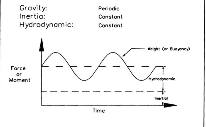
There are three contributions to the forces and moments measured by the balance in the model (see figure 10). The first is from the inertial forces and moments of the model itself, which vary with the model attitude and rotation speed. The second is from gravity (model weight) and buoyancy, which will vary cyclically over a revolution. Finally, there is the contribution from the hydrodynamic loads. The desire to reduce or eliminate all but the desired hydrodynamic forces had a great effect on the installation design.

Figure 10. Forces measured by the balance for constant rotation rate

A close-up of the model in the test section is shown in figure 11. The model cen-ter of rotation was chosen such that the model center of gravity would be as close to

Gravity:

Inertia:

Hydrodynamic:

)yoncy) Force or Moment Time

Periodic

Constant

(31)

Figure 11. Coning Motion Apparatus in the Test Section

the model rotation axis as possible. This reduces the inertial force contribution. Addi-tionally, reducing the differences in the model moments of inertia also decreases the body inertial moments (see Appendix B). As it turned out, the inertial forces were very small compared to the hydrodynamic loads.

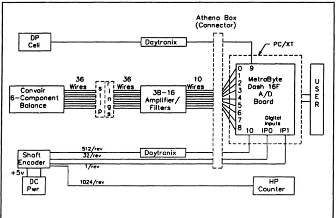
2.4 Data Acquisition and Reduction System

The data were taken with the stand-alone, microcomputer-based, data acquisition and reduction system shown in figure 12. The components will be described by their func-tional grouping.

(32)

Figure 12. Data Acquisition and Reduction System

2.4.1 Instrument Group

The instruments consisted of the 6-component balance, tunnel differential pressure (DP) cell, and shaft encoder. Their basic functions were as follows:

* Balance: 9-element (strain-gauge bridge), internal balance used for measur-ing the forces and moments experienced by the model

* DP Cell: Used for measuring test section velocity

* Shaft Encoder: 12 bit, natural binary encoder (BEI model C-14) used for model rpm, data trigger, and shaft position for static tests. The encoder out-puts a 0 to +5 volts square wave signal at frequencies from I/revolution to

Atheno Box (Connector) I I r, -i

ILeri

Doytronix r , I I 36 r

Con voir Wires I

6-Component E Bolonce R I-m u s

(33)

2048/revolution (2"). The 1/rev and 32/rev signals were used for shaft position, the 32/rev for triggering, the 512/rev for model rpm (computer input), and the 1024/rev for model rpm (counter input).

2.4.2 Amplifier/Filter Group

Signal amplification and filtering was accomplished by two sets of instruments: * 3-B Series (Type 3B-16): A nine module block of signal conditioners and

filters that filter and amplify the balance outputs to a standard ± 5 Volt ana-log signal. The modules had an upper cutoff frequency of 3Hz for filtering out high-frequency noise (a characteristic that caused considerable trouble later).

* Daytronix 9000 Series: Two modules were used: the strain gauge condi-tioner (9170) for boosting the DP output to a ± 5 Volts range, and the fre-quency to voltage module (9140) for converting the encoder 512/cycle output to a 0 to +5 Volt analog signal for model rpm.

2.4.3 Computer Group

The heart of the system was the IBM PC/XT personal computer. The PC had a MetraByte Dash 16F analog to digital (A/D) board installed for acquiring and convening the balance voltages to counts. The Dash 16F also read in outputs from the tunnel dif-ferential pressure (DP) cell and the shaft encoder. The analog portion of the board was set for a resolution of 2.44 millivolts (409.6 counts/volt). The board had a conversion time of approximately .0417 millisec./channel using direct memory access (DMA). This was a very important point which will be discussed in chapter 3.

(34)

The Dash 16F also was capable of reading in a digital signal through its digital input ports. This feature enabled the encoder to act as a trigger, using software to deci-pher the digital word read in from the port.

The PC/XT controlled the data taking process through software. Standard Project Athena laboratory routines were used for controlling the analog and digital sampling. The routines were incorporated into user-developed FORTRAN code. The major draw-back to using the FORTRAN routines was the increased time required to obtain an ana-log sample. The experimentally determined sample time was approximately .052 msec/channel, an increase of .0103 msec/channel over the calculated rate.

Finally, the PC stored and processed the averaged component (DC) of the signal and on-line presented the force and moment measurements. The time-varying signal was stored on magnetic media for later off-line processing.

Not connected to the computer, but used for seting the rotation rate was the HP (Hewlett-Packard) counter shown in the figure. The counter read directly off the shaft encoder and gave an accurate counts/sec output, which was then converted to RPM.

2.4.4 Slip Rings

The balance signals (millivolts) were taken from the rotating model reference frame to the fixed data system frame via a 50 ring slip ring assembly. The slip ring assembly (Airflyte model DAY-491-50) used was specifically designed for strain gauge measurements. As the experiment showed, the rings were very "quiet", passing little electrical noise to the amplifier/filters.

(35)

Chapter 3 Test Procedure and Tare Measurements

3.1 Balance Calibration and Check-out

The 6-component balance calibration was accomplished at Convair, prior to its installation in the model. A precise calibrating body was fit over the balance and then the assembly put in a calibration fixture. The fixture allowed for the accurate placement of loads and moments on the body, with corrections for deflection being taken into account. The calibration results were placed in a two inch thick binder containing information

nec-essary for using the balance. The information included:

* R-cal readings for all 9 channels (shunt resistor equivalent)

* Balance constants for the different combinations of roll moment and axial force gauges

* Plots of the response of the balance vs applied load (for applied axial, normal, and side force and roll moment)

The R-cal readings are merely voltage (counts) outputs for the balance channel being tested, with and without the shunt resistor switched into the circuit. The A voltage (counts) allows a second site to establish calibration ratios between the counts read en their A/D system and the equivalent readings on the Convair test bench. In this experiment, the ratio was set as:

R-calco,,v

Ratio- = 2.45

R-calmrr

The ratio varied by channel, however, the variance was small. The ratio calculated above shows that the Convair A/D system had approximately a factor of 2.45 better resolution than the system used in this study.

(36)

The balance constants were not used because of the simplified linear algorithm cho-sen for converting the balance readings to forces and moments. Several methods were available for doing this conversion, but the linear method was chosen for its simplicity and speed. Other methods available are described in References [12] and [13].

3.1.1 Data Reduction Model

Stevens Institute of Technology, Davidson Laboratories, developed the linear, 6! order method implemented in this study. In developing this linear model, Stevens had to fit the Convair calibration data and then compare the linear model performance against the more complex Convair algorithm.

The first step is to compute the 6x6 calibration matrix. The goal is to obtain a matrix of coefficients that accounts for the imperfections in the balance construction, which appears in the form of cross-talk, and yields the correct force vector. In other words, for a simple single, in-plane force, such as a normal force applied at the reference center, the detected force by the balance will consist of contributions from all 6 chan-nels:

6

Z = airi

i-I

where a, are the calibration coefficients and r, are the balance readings from the six

channels. For a generalized load application, the matrix equation is:

L =[A]R

(37)

where L is the load vector, [A] is the desired coefficient matrix, and R is the

correspond-ing balance readcorrespond-ing vector. Durcorrespond-ing the calibration done at Convair, several load vectors were applied while recording the associated balance reading vectors. This resulted in the following, overdetermined system:

Z, Zn a,, a,₂ a,3 a,4 a,, a,,6 Ni N1. M, Mn a2 a22 a23 a24 a25 a26 N2, N2

Y,...Y.

a, a32 a33 a34 a35 a Yll...Y1n

NI N, a4, a42 a43 a a45 a46 ,Y21 Y2,

K, K. a,, a52 a,3 a,54 a55 a,6 R2, R2 X, X, a61 a62 a6,, a6, a65, a X11 X1,.

where the subscripts refer to the loading condition. This equation can be rewritten as: [R]' [A]T= [L]r

The solution to this system is found by utilizing a least squares approach. This is equiv-alent to minimizing the Euclidean norm of

[R]' [A] T- [L]T

Davidson Lab has a standard program which, given a file containing the loads and results, carries out both the linear least squares fit and the matrix inversion to get the final coefficient matrix, [A] [12]. This matrix was then used to convert the balance readings obtained from the experiment into the force and moment data presented.

3.1.2 Balance Operation

The next logical step was to verify the correct operation of the balance. Successful completion of this portion of the experiment would give:

* A check of the data reduction method

(38)

* The balance axis convention * A check of the data taking system * Model weight and center of gravity

3.1.2.1 Weight Calibration and Axis Convention

The first experiment run was the application of known weights on the balance. Stevens Institute provided a collar attachment that fit around the stainless steel sleeve and allowed weight placement with the model set at ct, = 0 degrees and roll = 0 degrees. Weights were systematically placed on the collar and readings taken using the static FORTRAN code developed for these runs. Applied loads varied from .4 to

12 pounds. The resultant Z force was approximately 1.8 times the applied load. After much searching, the error was found in the coefficient matrix associated with refer-ence to the center of rotation. The transpose of the coefficient matrix had been used, causing the Z force error. The error was corrected, allowing the next step to proceed. The sign convention for the axis system was checked by first setting the model to 0", 0' and taking a measurement. This measurement became the "zero" file and would be subtracted from the subsequent reading. Next, a known (in sign only, not magnitude) force or moment was applied to the model and a set of readings taken. The difference between the second reading and the zero file produced the read sign of the force (or moment). The test showed the following axis convention:

* X: positive out model bow * Y: positive out model port side * Z: positive down

(39)

o M: positive for model bow down

* N: positive for model bow to port

(Bold typeface indicates non-standard sign convention.) To avoid further confusion,

the axis convention above was adopted for the test readings only. The test measure-ments would be presented as follows:

* Dimensional forces and moments: above, non-standard convention * Non-Dimensional forces and moments: SNAME axis convention as

pres-ented in the list of nomenclature.

3.1.2.2 Model Weight and CG

With the axis convention determined, the model weight and center of gravity were established. Two types of experiments were run, first, an inclining experiment, second, a simple set of roll experiments. In the first experiment, the model is set at 0' (pitch or x,), 0O (roll), a set of zeroes taken, and then inclined 2 degrees at a time (in pitch) with readings taken at each point. The weight is found from the relation

X = W sin(x,)

The X force is plotted against sin(ac). The slope of the plot is the model weight. The slope gave the model weight as = 10.3 lbs. Though the data plotted very linearly, the maximum X force measured was - .35 pounds. More emphasis was placed on the results of the following roll tests.

The next experiment consisted of a set of roll runs. First, the model was placed at either 0", 0* or 0", 90 (degrees roll angle). A set of "zeroes" were taken. Then the model was rolled 180 degrees and again sampled. The resulting readings gave the following results:

(40)

AM AK

* _{000, 180 Test: Z = 2(Weight), X, =} _{(W) Ycg =}₉ ₂₀₎

090, 270 Test: Y = -2(W), X, = - , Z," =,AK

Giving numbers:

* W 10.45 pounds

S XC, = .4 inches forward of center of rotation S Y cg = Z, = 0

As a measure of some confidence, the test data was re-reduced using the coefficient matrix referenced to the balance moment center (BMC). The results were nearly iden-tical. Additionally, the different components of the balance gave consistent results (i.e., Y force determined W = Z force determined W).

3.1.2.3 Temperature Effects

During this check-out phase, the temperature sensitivity of the balance was dis-covered. Because the balance is a large mass of metal, the temperature of the balance took some fixed time to stabilize. Even the small heat generated by energizing the gauges affected the balance outputs (significantly). A quick experiment was run where, with the model in air, the balance was energized and readings taken every few minutes. The first 15 minutes produced drifts of 2.5 lbs Y, 1.1 lbs Z, 1.9 in-lbs K, and

1 in-lb M. Over the next 30 minutes, the drift fell off considerably.

To counter this "warm-up" effect, the strain gauges were left energized during the entire experiment. The temperature sensitivity caused problems in the full-up data runs later because of the tunnel water temperature rise over run time.

(41)

3.2 Test Procedure

3.2.1 Test Logic

A coning motion test produces forces and moments from multiple sources. Three components discussed in Chapter 2 are weight (or weight -buoyancy), inertia and hydrodynamic. An additional "force" is the bridge offsets or zeroes. This fourth com-ponent is a function of temperature. The only force (or moment) of interest is the hydro-dynamic force. To this end, a test procedure had to be developed that accounted for each component and left the desired result. For this study, the desired result was both the time varying (or AC component) and the steady state (or DC component) hydrody-namic force. The basic test procedure was (starting with the model at the desired (a ):

A. Model in air

1) Take a set of readings at set angular positions around a 360' rotation. Mea-surements done every 11.25' starting at 0" and rotating in the positive (stan-dard convention) direction (by hand) to 348.75'(32 sampling positions). Store the raw counts for all 9 channels (100 sample sweeps/angular

position, summed to 1 point), both for each point (AC data) and the summa-tion of all 32 points (1 revolusumma-tion)/channel (DC data). Result: weight and offsets raw counts for that a, .

2) Conduct "wind-off' runs at same rotation rate (o) and direction as "full-up" runs. Sample all 9 channels (1 sample sweep/angular position) and store each raw counts data point. Sum raw counts for each channel over # of revolutions (usually 10) and store for processing with DC water run results. Result: weight, offsets, and inertia raw counts for that a, and co.

(42)

3) Subtract DC raw counts measurements in test A. 1 from the DC raw counts measurements in test A.2. Process the results for only the preferred 6 chan-nels. Result: inertia force for that a ond co.

4) Repeat A.2 through A.4 for each o, A.1 through A.4 for each a .

Note: Though not processed immediately, the weight and inertia vs angular posi-tion raw counts are stored and can be processed later for the inertial effect over a rotation cycle.

B. Model in water

1) After a "soak" period, usually overnight, repeat test procedure A.1, with the model in water and tunnel free stream velocity = 0. Result: weight - buoy-ancy, and offsets.

2) Establish tunnel test conditions (i.e., tunnel free stream velocity and model rotation rate). Conduct "full-up" run, recording 11 channels of data (9 bal-ance, 1 DP, 1 rpm) at each angular position and storing the raw counts. Sum raw counts for each channel over # revolutions for averaged (DC) component. Result: weight -buoyancy, offsets, inertia, and hydrodynamic raw counts.

3) Subtract DC raw counts measurements in test B.1 from DC raw counts measurements in test B.2 (9 balance channels only). Process averaged data for only preferred 6 channels, DP cell, and rpm data. Result: inertia and hydrodynamic averaged force (over # rotation cycles).

4) Subtract inertia force measurements corresponding to that Co and a. from the B.3 result. Result: Hydrodynamic force for those test conditions.

(43)

Note: Again, the time varying data are all stored as raw counts files for future processing.

The motivation behind the many decisions made in preparing this procedure is discussed in the following sections.

3.2.2 Code Development

At the core of the data taking was the FORTRAN software developed by the author (in conjunction with the routines developed by Glenn McKee of Stevens Institute, Davidson Labs). The form of the test procedure and its limitations dictated the form of the code. The critical issues considered were:

* Timing

* System capabilities

* Desired outputs (i.e., time varying and averaged forces)

3.2.2.1 Timing

The basic timing parameters considered were:

* A/D sample and conversion time for 11 channels * Model rotation rate

* Code loop execution time * # of divisions over a revolution

* Maximum allowed change in gravity vector over a sample sweep

The MetraByte Dash 16F specifications give an estimated A/D conversion time with DMA (Direct Memory Access) transfer of .04167 msec/conversion. For 11

(44)

channels, this works out to - .46 msec. The experimentally determined A/D conver-sion and transfer time = .052 msec/converconver-sion giving a total = .57 msec for 11 chan-nels. The importance of this is seen by looking at the maximum allowed change in gravity over a sample sweep.

Using a small angle approximation for the change in rotation angle over a sam-ple sweep, the following relation was derived:

AG = AO = .01rad (.57 deg)

for a maximum allowed change of 1%. At the maximum rotation speed of 200 rpm, this works out to .4775 msec. The data taking system used simply could not satisfy the 1% criteria (at 200 rpm). The actual AG for this study was = 1.2% (.68").

The time to execute one data taking loop lead directly to the # of increments that could be sampled over 1 revolution. Use of the shaft encoder as both a trigger and a position indicator (locating the 0* position) required several logic statements in FOR-TRAN. The logic allowed the code to read the digital word on the D/D input ports

and determine, 1) when to set 0", and 2) when to trigger a sample sweep. Embedded in the logic loop was the Project Athena Laboratory sampling routine for reading in and storing the A/D data. By running several loop timing versions of the data taking code, the time to execute the loop was found to be - 5.2 msec for an 11 channel sweep. Again looking at 200 rpm, the maximum number of increments in one revolu-tion that would allow the loop to execute and return for the next trigger pulse was 32. This allowed 9.375 msec for loop execution and return. 32 data points per rotation were felt to be adequate resolution for the purposes of the experiment.

(45)

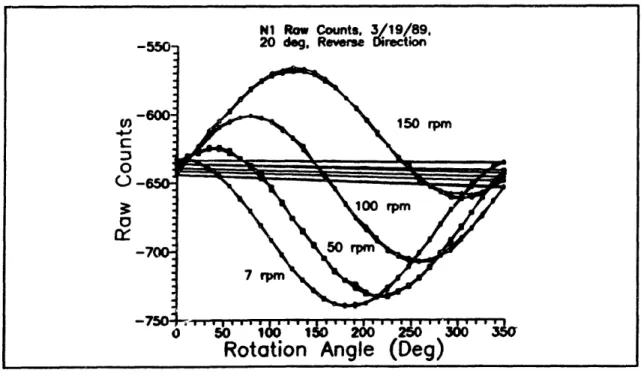
3.2.2.2 Desired Results

During the initial code development, the thought was to work directly with the individual raw counts data points for subtracting tares and converting to forces. The averaged force values would then be computed from these results. Unfortunately, upon actual data taking, a mysterious phase shift and amplitude drop off were noticed for all rotational speeds. The offenders in this case were the 3B-16 Amplifier/Filters supplied with the balance. This should have come as no surprise, especially when the

3 Hz upper cutoff frequency was known a priori. The phase shift can be seen

graphi-cally in figure 13. Fortunately, only the time-varying or AC component was affected, passing the zero Hz or DC component unchanged.

Figure 13. Phase Shift in Raw Count Data

This discovery initiated a flurry of code rewrite activity and caused a change in philosophy to working only with the averaged counts. To maintain the ability to work with the time varying data off-line, and to quantify (at least for one channel) the

Page 45

NI Row Counts, 3/19/89,

(46)

amplitude reduction and phase shift, a bode plot was made. The phase shift is shown in figure 14, the amplitude plot in figure 15. The best fit line for each was recorded

and stored for later use.

(47)

Figure 15. Amplitude Ratio vs Frequency

3.3 Tare Measurements

The test procedure delineated in section 3.2.1 accounts for the (W-B) and inertia effects. Though it is possible to account for these forces analytically, they were eliminated in a more straightforward manner by subtracting averaged (DC) measurements. The tare tests were run in air since, compared to water, the air acts essentially as a vacuum and doesn't influence the results. The general idea for the conduct of the tare measurements came from Reference [14].

Page 47

TIpIUGW fRati o v rs r ency , Chnonn, u 6th Order it 0.1 2n - - I7 2 115!S 1 1 .13 4.1 1 3 O 1 0' Q) e 0.1

a)

S. 4-,

-E-E~

0.0

rquency

1

4i

ii9

i i

4

ii

0.01 0.1e " Frequency (Hz _ _ I __ I AmwhýM-- Ck4:- - r- . - 4.-.A 0

(48)

3.3.1 Static

The static (o = 0) tares were very simple. The model (in water) was set at the desired qa, the roll angle set to 0, and a set of readings taken. This "zero" file accounts for the (W-B) and offsets for that qa. The tunnel test conditions were set and another set of readings taken. Subtraction of the two files left the desired static hydrodynamic load. A more thorough approach would have been to repeat this at several rotational positions and average the results. Because of time constraints, this was not done.

3.3.2 Rotational

The inertial loads can be calculated analytically, given the model mass, moments of inertia about the principle axes, and the location of the model CG. Additionally, these values must be assumed to not vary with rotation rate. If this course is pursued, then the following relations, derived in Appendix B, result:

* For the inertia forces (in SNAME axis convention): X5 = m ox, sin2 a

Y=0

ZX = -m o0oX sin a cos a

M, = -&2(I, - I.) (sin ao cos q,)

K,

=i

=N

0

(49)

X,w_ = -(W -B)sin a, cos ot

Yw- = (W - B) sin wt

ZWB = (W - B) cos a, cos otr

K=

W [yG cos a, cos (t - z sin (t]

M,= -W cos ot c [z sin ac +XG cos cc]

N=

W=W[x, sincot + yG sin a, cos Ot]

The same moment equations result for buoyancy by substituting -B for W and xB, yB, zB for xG, YG, G

There are several problems with using these relations directly. First, the model/sting combination deflects during rotation, causing the actual inertial loads to vary. Second, use of the weight and buoyancy relations would involve determining the offsets separately, rather than the more direct method of lumping them with the weight and buoyancy effects. Finally, the relations depend on accurately knowing the model mass moments of inertia, the CG, and mass. Errors in these quantities would reflect directly in the calculated forces and moments.

For this experiment, the deflection should be small due to the relatively small iner-tial forces at the maximum a, and co. As it turned out, the design of the model/sting minimized the inertia force contribution. The calculated and actual measured inertia forces for ca = -20" and -14" are shown in the following figures. Figures 16 and 17 are for the -20' setting, figures 18 and 19 for the -14" angle. The moment measurements have been corrected for sign to conform the standard convention.

(50)

X and Z Imertia Forces Caulated and and Mesured

Alpha - 20 Degrees (i)c 00 0- o-Force Force Force Force SMeasuredColculated)

Measured

ulate)

50 i6•"

10

200

250 Rotation Rate (RPM)

Figure 16. X and Z Inertia forces, 20'

M Wertl Moment

o Calculated and Measured

e Alpha w 20 Degrees

0

-Figure 17. M Inertial Moment, 20'

go" X Loe Z T0o C 4-a C' E 0-Rd (et rt)

ed

50 100 . . 0 200 250

Rotation Rate (RPM)

_ I I IPFmrrq rTqrrrli F

(51)

X and Z bterio Forces

Caculated and Measured

Aph - 14 Deogree a atee* X Force meeee Z Force O n•E Z Force .u5~l.'~uuI'.*I~~~~l III 50 100

Rotation Rate

(Measured) (Calculaed) Measured)

Calculated)

150 200

(RPM)

Figure 18. X and Z Inertia Forces, 14'

M Inertial Moment SCaolculated and Measured

Figure 19. M Inertial Moment, 14'

Page 51 0 0)_O O la.. -_-· '0.-C: .0i 0I O0 9) -C (u)0

4.'w-7c

it)

0

50

100 0so

200 Rotation Rate (RPM)

I