Design, analysis, and control of a bill deskewing device for automated teller machines

DESIGN, ANALYSIS, AND CONTROL OF A

BILL DESKEWING DEVICE FOR

AUTOMATED TELLER MACHINES

Ross Bennett Levinsky

S.B., Aeronautical/Astronautical Engineering

Massachusetts Institute of Technology (1989)

Submitted to the Department of Mechanical Engineering in partial fulfillment of the requirements for the degree of

Master of Science in Mechanical Engineering at the

Massachusetts Institute of Technology January 1992 © Massachusetts All Institute of Technology 1992 rights reserved Signature of Author

Department of Mechan(?lal Engineering January 17, 1992 Certified by Accepted by I I X \ - -Harry West Thesis Supervisor MA~ftTS INTT

'RA .ati6 "17as INS TIrTUTE OF TE.!fi)j OGY

F 'I ;: 0 1992

Ain A. Sonin Chairman, Departmental Graduate Committee

Design, Analysis, and Control of a

Bill Deskewing Device for

Automated Teller Machines

Ross Bennett Levinsky

Submitted to the Department of Mechanical Engineering on January 17, 1992 in partial fulfillment of the requirements for the degree of Master of Science in Mechanical Engineering

Abstract

A prototype device has been constructed to straighten banknotes that are skewed with

respect to their direction of travel in an automated teller machine. The design requirements were

high reliability, low hardware cost, low control complexity, and infrequent need for adjustment; they were met with a simple system consisting of four optical sensor pairs, two

solenoids, and a tunable open-loop controller. To demonstrate the modeling of such a system, a simplified analysis of note handling by frictional contact is presented and numerically applied

to the deskewing process. This modeling technique can be used to gain a qualitative

understanding of how changing design parameters affect machine performance. A conceptually simple tunable open-loop controller, based on a lookup table, has been implemented to improve

robustness of the deskewer by compensating for changing environmental conditions and note

quality. It is shown that experimentally-observed constraints on the behavior of the deskewer

allow a stable tuning algorithm to be developed; in addition, the simplicity of the controller concept allows a low-cost control circuit to be used. Experiments indicate that the machine

reduces note skew to within design limits.

Thesis Supervisor: Dr. Harry West

Acknowledgements

I am indebted to Harry West for the opportunities to work on this project and to travel to

Japan. His counsel on matters technical and not-so-technical was invaluable. I am also grateful

to the Omron Corporation for funding what was initially an open-ended, speculative project

through to its current level of maturity.

Many thanks go to my friends and fellow engineers at Omron: Hiroyuki Nishimura (the motivating force for this project at Omron), Ryuichi Onomoto (who taught us about note handling and collaborated in the design of the deskewer), Ichiro Kubo (who explained the sensor circuits used in Omron's money-handling equipment), and Yoshimasa Sugitate (who

designed and helped in the analysis of a new note feeder). They made both my work on this

project and my stay in Japan tremendously positive experiences. I look forward to working

(and playing) with them for many years to come.

Jack Kotovsky, who was a member of the design team and who built the prototype for his bachelor's thesis, did a fine job. His work has withstood many hours of experimentation and abuse. Henry Dotterer followed Jack on this project and, on his own, did the first experiments on learning algorithms (wholly separate from those described in this thesis). Matthew Selick, provided assistance in coding, guidance through the maze of Turbo C, and ceaseless help in divining the mysteries of interrupts on the IBM PC. Without him, the deskewer control would never have reached its current level of sophistication. Nathan Delson also made his experience

with interrupts available to me at the beginning of this work.

Thanks to the many people who made easier what was occasionally a difficult experience; to

my friends, for listening to me complain about note-handling and for accompanying me on forays into the world of late-night food in Boston; to Peter Robeck, for his time, patience, inspiration, and friendship; and most of all, to my parents, for their love, support, and

Table of Contents

Acknowledgements ...

... .6

1 Introduction

...

...

10...

1.2 Basic Technology of Bill Counting . ... ... ... 10

1.3 Skew

...

..

...

...11

1.4 Design 2onsiderations ... 13

1.5 The Deskewing Machine ... ... ... 15

1.6 Modeling and Control Problems .. .... .. ... 17

1.7 Thesis Overview ... 8...1

2 Analysis of the Deskewer ... ... ... 19

2.1 General Case of Coulomb-Frictional Contact ... 19

2.2 Deskewer-Specific Equations ... ... ... 21

2.3 Example Solution of Deskewer Equations ... 23

3 Control of the Deskewer ... 26

3.1 Mathematical Formulation of the Deskewer Control Problem ... 26

3.2 Control Schemes ... 28

3.3 Creation of the Control Mapping ... 30

3.4 Qualitative Behavior of the Deskewer . . ... 31

3.5 Convergence at One Input Skew . ... ... 34

3.6 Multiple Input Skews in One Bin ... .. ... ... 37

3.7 Error in Deskewing Performance ... 39

3.8 Limitations of the Analyses ... ...42

4 R esults ...

...

45

4. 1 Implementation of Deskewer Control ... ... 45

5 Conclusions ... 50

Appendix A - The Yen ... 53

Appendix B - The Deskewer ... 54

Appendix C - Feeder Analysis . ... ... ... 59

C.1 Origin of Model ... 59

C.2 Direction of Frictional Force Vector ... 59

C.3 Feeder Gap Calculation ... 61

C.4 Yen Model ... ... 62

C.5 Motion of the Note ... 63

C.6 Example Solution of Feeder Equations ... 64

Appendix D - Implementing IBM-PC and PC/AT Interrupt Control ... 66

D.1 General Information ... 66

D.2 Initializing Interrupts ... 67

D.3 Ending the Program ... 68

D.4 Interrupt Functions ... ... 69

D.5 Sample Program ... 70

Appendix E - Deskewer Control Program ... 71

E. 1 Constant.h ... 72 E.2 Globals.h ... 73

E.3 Main.c ...

...

74

E.6 Interpt.c ...

81

References

...

84

List of Figures

1.1 Simplified Sketch of Feed Roller . ... ...11

1.2 Definition of Skew ... 12

1.3 Selected Design Options . .. . ... ... 14

1.4 Simplified Conceptual Sketch of the Deskewing Machine ... 15

1.5 Sketch of Deskewing Action ... 16

2.1 Small Plate Element Sliding on Moving Surface . . ... 20

2.2 Direction of Friction Vector ... 21

2.3 Plan View of Deskewing System ... 22

2.4 Simulation Results for Varying Pin Position (P) ... 24

2.5 Simulation Results for Varying Solenoid Position (S) . ... 25

3.1 Sketch of Skew vs. Time ... 27

3.2 General Form of Skew-Timing Function ... 29

3.3 General From of Tunable Open-Loop Controller . .... ... ... ... 29

3.4 Initial Note Skew is Binned . ... 30

3.5 Control Action Comes from Bin ... 31

3.6 General Form of F(0in,T) .3... ... 33

3.7 General Form of G(in) ... 33

3.8 Single Bin of G(in) ... 34

3.9 Bin Value is Correct at One Input Skew ... 39

4.1 Experimental Graphs of F(Oin,) ... 47

4.2 Experimental Graph of Output Timing in 19.80 - 20.40 Bin ... 49

A.1 Y10000 Note Characteristics ... 53

B. 1 Test Fixture and Deskewer Closeup ... 55

B.2 Main Structure of Deskewer ... 56

B.3 Sensors and Solenoids ... 57

B.4 Side Plate of Deskewer ... 58

C. 1 Plan View of Feeder Model...60

Chapter 1

Introduction

1.1 Historical Background

Since 1969, the Omron Corporation of Japan has designed and produced various types of cash-handling equipment, from change dispensers to automated teller machines (ATM). The technologies used have been experimentally tuned to a very high level of sophistication over time; by 1990, Omron's most advanced model, the HX-ATM, reliably operated at a transfer rate of ten notes per second.

During the late 1980's, though, engineers at Omron became convinced that they needed to expand their analytical knowledge of the note-handling process in order to increase transfer speeds and improve reliability. To reduce the need for expensive human service, they also wanted to begin incorporating self-adjusting mechanisms and mechanical error-correction systems into their designs.' With those goals in mind they entered into a research project with the Mechatronics Design Lab of the Massachusetts Institute of Technology.

1.2 Basic Technology of Bill Counting

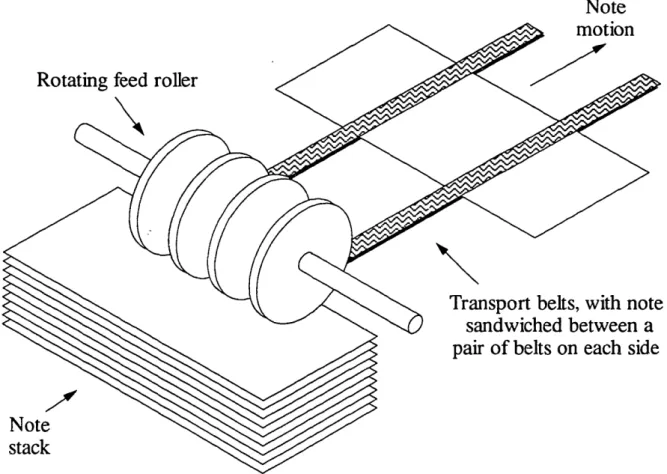
The bill-handling technology used by Omron is similar to that employed by other major Japanese manufacturers of such products (Hitachi, Fujitsu, Oki, and Toshiba). In contrast to ATM in America, where cash to be deposited is first placed in an envelope, ATM in Japan directly input bills from the customer. The notes are slid from the top of the deposit stack by a rotating feed roller (see Figure 1.1) and carried through the machine by rubber transport belts that "sandwich" the notes. Through a complicated series of belts and sensors the bills are validated, counted, and stacked in cartridges during a deposit cycle, and fed, again using rotating-feed-roller technology, out of the cartridges during cash withdrawal. While the machines examined during this project were built for the Japanese market (and were thus sized

1Information about Japan's ATM market, Omron's machines, and Omron's perceived need for analytical models came from a series of discussions with key Omron personnel over a two-year period. These people included, but were not limited to, Hiroyuki Nishimura, Ryuichi Onomoto, Ichiro Kubo, and Yoshimasa Sugitate.

to handle yen), Omron uses near-identical technology to produce cash-handling equipment for other Asian countries.

This principal failure mode in Omron's machines is jamming. Typically, a note becomes stuck at a fork in the travel path while the notes behind it continue to move, causing one or more bills to crumple before the machine's optical sensors detect the problem and stop the transport mechanism. The exact causes of failure are difficult to pinpoint because the failure rate is so low - the only statistics Omron has are taken from in-service operation. It is has not

been possible to observe enough failures in the controlled factory environment to adequately

de:ermine all causes of jamming.

Note

Rotating feed roller

Note

stack

Figure 1.1: Simplified Sketch of Feed Roller

1.3 Skew

therefore decided that the initial approach to improved machine reliability would be to correct skewed notes in transit. Skew (see Figure 1.2) is defined as a note's angular deviation from the correct travel position in which its short side is parallel to the direction of belt travel. The

spacing between a skewed bill and its two surrounding notes (leading and trailing) is incorrect; this can cause jamming at forks in the travel path.

Note /

ing

'

This note is

skewed

Figure 1.2: Definition of Skew

Earlier research in this project investigated the origins of skew. It has been found that skew

occurs at the very beginning of the feeding process, when the note is accelerated by the slipping frictional contact of the feed roller. If a note enters the roller with one corner leading (slightly skewed), the frictional forces are initially applied at that corner, causing a torque that rotates the bill and increases its skew angle. This effect has been predicted by numerical simulation (see Appendix C) and confirmed with high-speed video. In addition, if the feed roller does not exert even pressure at all points along its axis, the note skews. This occurs

because the frictional feeding force on a given area of the note's surface is proportional to the pressure that the roller applies at that area; when the pressure is not uniformly distributed along

machine maintenance when technicians perform feed-roller pressure adjustments based on a machine-accumulated record of each deposited note's skew as it exited the feeder. An

asymmetrical distribution of skew indicates that the roller pressure is uneven.

1.4 Design Considerations

During the course of discussions with Omron, four major design requirements were formulated for the deskewer (the working name for the skew-correcting mechanism). They

were:

1. High reliability. The current generation of Omron machines is approaching a failure rate (where failure is defined as any problem requiring human intervention) of 1 in 5000 notes; addition of the deskewer should improve, not degrade, this figure. The machines are designed to accommodate skews of up to 80 without jamming, so the deskewer must

be consistently capable of reducing skew to less than 8° .

2. Low cost. Although ATM are complex their profit margin is small; inexpensive sensors and actuators must be used.

3. Computationally-simple control algorithm. The CPU is already severely taxed in

present-generation machines, so it is desirable to design a deskewer that requires little

computation to properly straighten notes.

4. Low need for adjustment. ATM are serviced infrequently by expensive trained personnel, so a long-wearing or self-adjusting mechanism is necessary.

Possible deskewer designs were classified into three broad types:

1. Geometric-constraint. A mechanism is incorporated that firmly grasps the note and deskews it, possibly while also continuing the note's travel through the machine. An

example of this method, shown in Figure 1.3, is a scheme in which there is a section of

the ATM that transports the note by motor-driven rollers (no rubber belts). By giving the rollers slightly different angular velocities, the note simultaneously deskews and continues its movement through the machine. This method is likely to produce excellent deskewing performance and low note wear but has the drawbacks of high inertia in the

transport rollers and the need for active control of the motors.

diverse as a directed airstream and a robot finger dragging on the top surface of the bill. The difficulties are that a compressor is required for schemes involving air, some form of

force control is required for mechanical systems; and note wear may be high.

3. Hybrid Geometry/Force. These designs have a mechanism that stops a point of the note (geometric constraint) and allows the frictional force applied by the moving transport

belts (force application) to deskew the note. Two examples are shown in Figure 1.3; the

blocking rods descend into the travel path and straighten the note when its leading side

collides with one of the rods, while the solenoids pin a single point on the leading side of

the note and allow the rest of the bill to rotate about the pinning point. The advantages of these schemes are the low cost and low inertia of the stopping elements, and the simple (stopper is either on or off) control. Possible problems include note buckling or

crumpling and high note wear.

Figure 1.3: Selected Design Options

Both the active roller geometric-constraint design, because it showed potential for both

excellent performance and low note damage, and the two hybrid geometry/force methods

(solenoids and blocking rods), because they were inexpensive and simple to control, were

selected for detailed consideration. The hybrid methods were eventually viewed as more viable because of lower component costs than the geometric method and uncertainty as to whether the rollers in the geometric-constraint design could have their angular velocities precisely altered at

Designs

Active rollers

Blocking rods

Solenoids

Characteristics

Control Complexity High Low Low

Note wear Lowest Highest (crumpling) Moderate (belt sliding)

Actuator inertia High Low Lowest

High need

Higls need Yes No No

for adjustment?

Cost High Low Low

frequencies above 10 Hz (This figure is actually an underestimate for ten notes/second operation, because a roller's speed must be adjusted and stabilized in the interval between notes. This implies a minimum response frequency above 10 Hz.).

Discussion ith Omron's engineers revealed that they had independently tried an error-correction scheme similar to that of the blocking-rod system and had found that the rods crumpled an unacceptably high percentage of bills; wrinkled notes did not have enough stiffness to withstand the stresses of suddenly impacting a barrier in the travel path. So, the solenoid deskewing technique was finally chosen as the concept to be implemented in the

prototype machine.

1.5 The Deskewing Machine

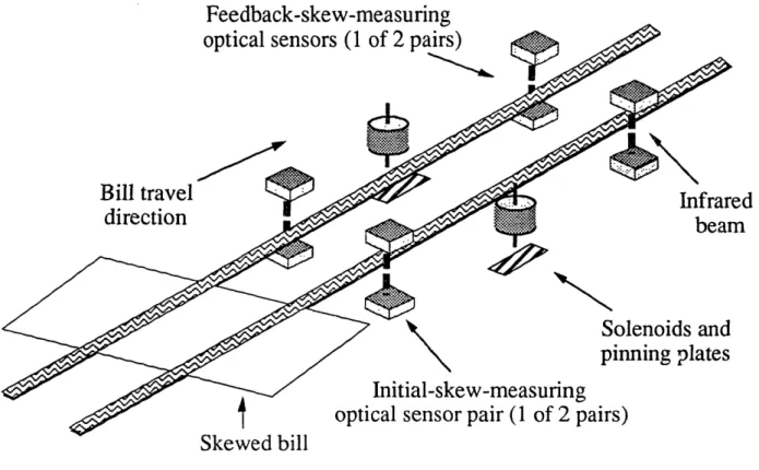
A conceptual sketch of the deskewer prototype is shown in Figure 1.4. Detailed drawings are presented in Appendix B, while additional information on design alternatives and

construction has been documented elsewhere [Kotovsky 1989].

Feedback-skew-measuring

Bill travel

direction

_n

pin

Initial-skew-measuring

optical sensor pair (1 of 2 pairs)

Skewed bill

Figure 1.4: Simplified Conceptual Sketch of the Deskewing Machine

z

The note's skew is determined by measuring the time difference between obscuration of the

left and right initial-skew optical sensor pairs, as detailed in Section 4.1. The measured skew,

along with belt velocity (measured by a tachometer), is used to select a "wait time" and a "fire

time" for the solenoids. The waiting period is programmed into a countdown timer that inhibits control action until the trailing half of the note is under the solenoid core (to reduce problems with buckling); at that time a second countdown timer containing the fire time begins decrementing and activates the solenoid, pinning the bill for the duration of the fire time. A

very small area of the note is pinned against a steel plate (below the travel path) by the extended solenoid core so that the note is only free to rotate about the solenoid's contact point (Figure

1.5). The transport belts slip over the note's surface and generate a frictional force which rotates the note about the pinning point, thus reducing the skew. If the fire time has been

properly selected the solenoid releases at the exact moment that the note is fully deskewed, and the note resumes its normal travel. Depending on note velocity and skew, fire time ranges from

approximately 10 to 50 milliseconds.

motion

Right-side solenoid fires and holds bill to pinning plate.

Belts on both sides continue to move, dragging bill about axis of right-side solenoid.

1.6 Modeling and Control Problems

The detailed modeling of frictional-contact note-handling machines presents three fundamental difficulties. First, the Coulomb friction model (frictional force is proportional to normal force) is empirically derived and does not model the stick-slip behavior that can occur

when a portion of the bill touches a surface such as the feed roller or the transport belts.

The second problem is the extreme variability in note quality encountered during actual

operation. Notes are nonisotropic because they have usually been folded; at a crease they bend

more easily in some directions than in others. This contrasts with the usual simplifying assumption that a note is an isotropic plate, and makes buckling analyses very difficult. This is a significant problem in sophisticated models of the deskewer because poor selection of the solenoid contact point has been experimentally observed to yield various forms of note crumpling; the behavior of each note depends on its overall condition (stiffness decreases with

increasing wear) and particular pattern of creases.

Third, even with a considerably simplified system model the resulting note-motion equations involve complex multidimensional integrals with time-varying limits of integration, as shown in Chapter 2. These equations are usually solved numerically, and are thus principally used to examine the qualitative effects of the variation of design parameters on

machine performance.

In addition to the basic difficulty of getting a plant model, control of the deskewer is

challenging because the required fire time for a given skew can vary according to such factors

as humidity, which is believed to change the note's mechanical properties, and belt wear,

which affects both the coefficient of friction between belt and yen and the overall belt tension. This performance variability is not a problem if each note's skew is continuously measured and

some type of individual-note closed-loop control effected, but such a system is difficult to

implement because of the high speed (ten notes/second) of machine operation and the lack of an

inexpensive sensor for continuous measurement of skew.

While a closed-loop controller offers good performance, it violates the cost and low-control-complexity design requirements; "closing the loop" on a particular note is much more

difficult and costly than simple open-loop solenoid programming, in which the fire time is a

function of a single measurement of incoming skew. In contrast, control hardware for the open-loop controller is simple and inexpensive, consisting of timers and low-cost optical sensor pairs that measure the incoming-note skew, and timers that hold the solenoid wait and

fire times. The drawback of the open-loop controller is that its fixed mapping between incoming-note skew and solenoid fire timing does not allow for changing deskewing times due

to environmental, machine wear, and note wear effects.

Each control scheme has its advantages. An open-loop controller is desirable because of its computational simplicity and inexpensive sensors, while an individual-note closed-loop controller more effectively handles changing machine and note conditions. The ideal controller would combine the simplicity of open-loop with the robustness of closed-loop. The compromise that has been chosen is a tunable open-loop controller in which the open-loop control law is adjusted in response to measured deskewing performance. Feedback is not effected on any single note while it is deskewing, but a measurement of the success of the

process, taken as the note is exiting the deskewer, is used to alter the control mapping and thus

change the solenoid fire timing for all future notes. The implementation of such a scheme is

explained in Chapters 3 and 4.

1.7 Thesis Overview

This thesis describes both the frictional-contact analysis and the self-tuning controller that have been applied to the deskewer. A simple analytical model of the system is presented in Chapter 2, along with sample computer solutions. The concepts underlying the tunable controller and a derivation of the tuning rule are explained in Chapter 3. Results of the implementation of the controller on the prototype deskewing hardware are given in Chapter 4.

Chapter 5 summarizes the project and points out directions for further research.

Appendix A gives the dimensions and mass of the Y10000 note, which is the most commonly handled note in Japanese ATM. Appendix B has more detailed views of the deskewer, along with parts lists. Appendix C applies the analytical methods developed in Chapter 2 to a model of the rotating-roller note feeder. A step-by-step procedure for utilizing interrupts on the IBM-PC and PC/AT is set forth in Appendix D. Appendix E lists the deskewer control program.

Chapter 2

Analysis of the Deskewer

2.1 General Case of Coulomb-Frictional Contact

The fundamental model for many bill-handling tasks is that of a machine surface interacting

with the note through frictional contact. This is the case in the feeding process, in which the

feed roller slips with respect to the note's surface and accelerates the bill into the travel belts. It

is also the reason that the deskewer is able to straighten bills; the belts slide over the yen and exert a moment which rotates the note about the solenoid's pinning point. Because sliding frictional contact is so fundamental to the note-handling process it is useful to consider the

general case of Coulomb-frictional contact (in which the frictional force is linearly proportional to the contact force).

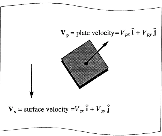
Consider a small sliding plate in contact with a moving surface, as in Figure 2.1. The plate

can be viewed as a differential element of the yen, while the moving surface can be considered

a sliding belt or rotating feed roller. Coulomb's Law of Friction describes the magnitude of the frictional force as proportional to the normal force between plate and surface (with proportionality constant g, the coefficient of friction) and the direction of the frictional force as

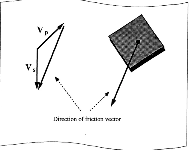
that of the relative velocity between plate and surface (Figure 2.2):

Magnitude of frictional force =IF = IFnI (2-1)

Direction of frictional force = V - Vp = (Vs, -Vp) i + (Vsy -Vpy)j (2-2)

To get the complete expression for frictional force on the plate, the force direction vector is normalized into a unit vector. This leads to:

Normalized Ff direction= Vs - V (VS, -V, )i+(Vsy -Vpy (2-3)

V

=

plate velocity

= Vp

i

+ Vpy j

V = surface velocity =Vsx i + Vs

j

Figure 2.1: Small Plate Element Sliding on Moving Surface

The frictional force vector is simply the frictional force's magnitude multiplied by the unit

direction vector:

F

=

lFd

V

Vsx

-

(

-VPx)

(Vy -VPY

+

)

j(2-4)

s - n (Vx-px )2 +(Vsy -Vpy)2

Equation (2-4) is the general expression for sliding-friction force on a non-rotating element. A note can be thought of as many tiny elements connected together, each with a slightly different velocity vector (due to the entire note's rotation). If the entire region of contact

between the note and the surface is integrated, the total force acting on the bill can be found,

and the note's motion can be predicted. The surface's definition changes according to the specific analysis; for the feeder it is the feed roller area in contact with the note, while for the

deskewer it is the belt area in contact with the note (neglecting the area pinned by the solenoid).

__ _____

Appendix C analyzes a feed roller system using the same Coulomb-friction model, but with a slightly different derivation of the note's equations of motion.

VP

Vi

Direction of friction vector

Figure 2.2: Direction of Friction Vector

2.2 Deskewer-Specific

Equations

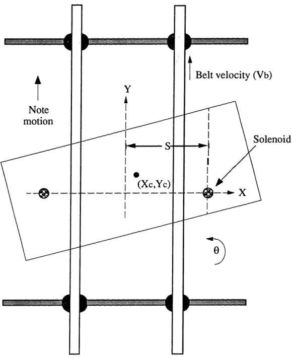
Figure 2.3 is a plan view of the deskewer prototype. Equation (2-4) can be applied by

considering the moving belts to be the surface and the yen to be a connected collection of small

plates. With the coordinate system oriented as shown, V,,x, the x-direction component of the

surface velocity, is zero and Vsy, the y-direction component of the surface velocity, is set to Vb, the belt velocity:

Vsx = 0 (2-5)

Vsy = Vb

---

---I

Note

motion

)lenoid

Figure 2.3: Plan View of Deskewing System

Because the note is pinned by the solenoid and rotates around the pinning point, it is convenient to express the note's surface velocity as a function of surface position and rotation

rate about the pinning point. If co (= 0) is the angular velocity of the note about the pinning point, (X, Y) is the position of an arbitrary point on the note's surface, and S is the solenoid displacement from the centerline of the travel path (as in Figure 2.3):

Velocity of note point (X,Y) = -coY - o(S-X)j (2-6)

A

Thus: vpx =' -ty (2-7) Vpy = -o(S-X) Substituting into (2-4): DeskewerFf = p Fn toY i + (Vb + w)(S -X))j (2-8) V(oy)2 _{+ (Vb + Co(S-X))}2

The note is viewed as a connected group of small plates, so the normal force is more properly treated as a normal stress (assumed constant over a single plate due to its small size)

multiplied by the area of a plate.

IFnl = o (X,Y) dX dY (2-9)

The standard differential equation for a rotating rigid body is now applied. I is the moment of

inertia of the note when rotating about a given solenoid pivot-point position, and R, the region

of integration, is the contact area between the belts and the note. It varies with time.

10= / (X,Y) i +V ( S -X) dX dY (2-10)

R/(Y)

2

+

(Vb

+

t(S-X))

The remaining difficulty is the prediction of the normal forces between the note and the belts. This problem is complex due to the high flexibility of the belts and the note, so for numerical investigations the normal stresses are generally assumed to be constant over the contact area.

2.3 Example Solution of Deskewer Equations

It can be seen immediately that (2-10) is difficult to solve analytically even with a simple, constant expression for A, so a computer simulation has been written to numerically solve the

equation. For simplicity, the program ignores buckling of the bill by assuming the note to be a

rigid plate. First a spacewise integration is performed over the yen-belt contact area to determine the force on the bill, and then a time-domain integration is performed to find the motion of the

bill over a small time interval. The fineness of the integration steps is then adjusted until consistent results are obtained. Predicted performance (in the form of necessary solenoid fire

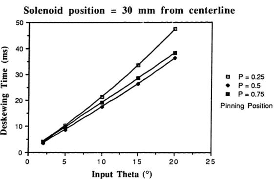
time vs. input skew) has been obtained for a number of different machine configurations, and a sample result graph is shown below in Figure 2.4.

This graph displays the slight variation in hold times required for different positions, relative to the leading edge of the bill, of the solenoid pinning point. "P" refers to the normalized distance back from the leading edge; P=O means the pinning point is at the leading edge and P=1 indicates that the pin occurs at the trailing edge. The lateral solenoid position (S) and belt speed (Vb) are fixed in all cases shown, with the solenoid position at 30 mm and the belt speed

at 1 m/s. Note properties are those given in Appendix A.

Solenoid position = 30 mm from centerline

D U -, 40-E E 30o-*e 20-10 W

10-0

Figure 2.4: Simulation Results for Varying Pin Position (P)

Experimental evidence indicates that this graph is qualitatively correct. Pin positions of P<0.5 tend to require longer hold periods for adequate deskewing, while those, towards the trailing edge need less time. As an additional advantage, the trailing-edge positions have been observed to cause less note buckling than those towards the leading edge. When the pin is

located towards the rear the deskewing force provided by the belts acts to tension the bill, thus

reducing buckling problems.

Figure 2.5 shows a graph similar to that in Figure 2.4, except that the pinning position is now fixed at P=0.75 while the lateral solenoid position (S) is varied from 30 mm to 65 mm. The simulation indicates that the required deskewing time is slightly affected by solenoid

0

--position, with S=65 mm consistently requiring the most time. The biggest variation in timing occurs at an input skew of 20°_{, and is 4.4 milliseconds (between the 65 mm and the 50 mm}

positions). This effect is notable because the feeding process normally causes slight (up to approximately 10 mm) variation in the lateral position of notes. Two bills with identical input skews but horizontally-offset positions in the transport belts are entering two slightly different deskewing systems, distinguished by a difference in S. The notes thus require different deskewing times.

P = 0.75

Figure 2.5: Simulation Results for Varying Solenoid Position (S)

W ._ E ._ W 19 Q, u: ----.--- r-- -, , , .· . !

-___I -

--- I __- -- 1__ - _

Chapter 3

Control of the Deskewer

3.1 Mathematical Formulation of the Deskewer Control Problem

A very large class of systems can be described by equations of the form (3-1), where all terms are vector-valued.

: = A(x)+ B(u) (3-1)

In such a system the fundamental control problem is to choose a control action u (as a function of time) that is guaranteed to cause the state vector x to converge to a desired trajectory. There may be other requirements involving convergence time or cost of control, but

the basic necessity is that u yields a stable, convergent system.

If (3-1) is rearranged as follows:

x- A(x)= B(u) (3-2)

an essential feature of this type of system can be seen - it has only one set of equations to describe its behavior, regardless of the control action. As long as the system's behavior stays within the bounds of the modeling assumptions, the function u does not change the overall form of the system equations. Different u will lead to different time evolutions of x, but the

theoretical framework will remain that of (3-2).

The deskewer is fundamentally different from systems described by (3-2) in that the

application of the control action (the firing of the solenoids) completely changes the form of the

system equations. Again taking 0 as the note skew and o (= 0) as the note angular velocity

about the pinning point, the system equations can be stated as follows. When no control action is applied (solenoids are inactive):

D= w=0

(3-3) = constant

When control action is applied (solenoids are tirud), equation (3-4), which is a recasting of (2-10) in the form of (3-2), holds.

=

/Ij=

u.

R

/(woY)

2

+

(Vb

+

o(S-X))

2

(3-4)

Figure 3.1 is a qualitatively-correct graph of 0 versus time since measurement of skew. The

programming of the deskewer is a question of when and how long to switch the system model from (3-3) to (3-4).

e

Skew measured

at time = 0

Solenoid fires at this time

Solenoid lifts at this time

F,

. . I

,., . , I

S~~~~~~ ... ,.... ."

-I

Eq.

(3-4)

obeyed

here

.

Eq. (3-4) obeyed here -"'..

Il

Time

Eq. (3-3) obeyed here

Figure 3.1: Sketch of Skew vs. Time

If a system of the form shown in (3-2) is controlled in a bang-bang fashion, its equations resemble those of the deskewer. The similarity is not exact, though, because a bang-bang controller is typically capable of both positive and a negative control action; if the task is

position control of a motor, for example, the bang-bang controller is able to apply both positive and negative voltage (usually of the same magnitude). The deskewer is a "one sided" system in

...':·I:: ....:'.:..·:. ..: ·::· ;·:. :I ·.. -. .·:· ··· ··: ·:I·;: '::: .`.:·'·'· :. ··'..·i I ·· ..- .:··....·' ·I' · _ . .w.. ... . . .. . ... ... .. L --- ... -- -- --~ - . -_ _-

--that the control action is either on or off, with no possible negative action. An analogous

system is that of a motor which has only one input voltage and an on-off switch.

3.2 Control Schemes

The time at which to switch to equation (3-4), which is the selection of the solenoid waiting time, can be calculated in a very simple fashion. As noted in Section 2.3, the bill experiences minimal buckling when the solenoid pinning point is located towards the note's trailing edge. For a desired pin location the correct wait time is easily calculated with knowledge of the distance between the skew-detecting sensors and the solenoids, the bill's skew, and the belt velocity (measured from a tachometer attached to one of the deskewer's rotating shafts). In practice the pinning point is generally located on the back 30-50% of the bill, where it causes no buckling problems.

Selection of the total solenoid firing time (t - tf) is a more challenging problem for the reasons discussed in Section 1.6. There are many possible methods for selecting the proper

timing, with the most basic distinction being that between closed-loop and open-loop control.

A closed-loop controller continuously measures the skew of the note while it is pinned and retracts the solenoid at the appropriate time. The advantage of this method is that it dynamically

produces the correct deskewing times and thus accounts for machine wear, changing note quality, and varying environmental conditions without requiring a detailed understanding of how these factors affect deskewing performance. The disadvantage, as pointed out in Section 1.6, is the difficulty and cost of measuring skew continuously. While arrays of optical sensors

could potentially give a continuous report of note skew, they are much more expensive than the simple phototransistor - infrared LED pairs that can be used to take a single measurement.

The open-loop scheme simply programs the solenoids on the basis of measured incoming

skew and then ignores the note until after it has left the deskewer, at which point the outgoing

skew may be measured for later reference; for example, in the tunable open-loop controller discussed below, the outgoing skew information is used as feedback data to adjust the solenoid fire timing. This method has an appealing simplicity, makes low demands on the skew

sensors, and is straightforward to implement in hardware. However, the simplest open-loop

controller, in which there is a static mapping between incoming skew and solenoid fire time,

has the disadvantage of not adapting to changing note and/or environmental conditions.

Exceptionally worn bills are treated exactly the same as fresh, crisp notes, and no distinction is made between humid and dry weather.

Solenoid

fire time

-r

Incominpg A

Figure 3.2: General Form of Skew-Timing Function

Thus, this project has focused on the creation of a control scheme that possesses both the

hardware simplicity and low cost of an open-loop controller and the robustness of a closed-loop

system; it is described as a tunable open-loop controller. It creates a mapping, similar to that depicted in Figure 3.2, which is altered in response to measurements of the deskewer's performance but which is not changed during the straightening of any particular note. The note's outgoing skew is recorded and is used to adjust the mapping after the note has exited.

The general form of the controller is shown in Figure 3.3.

Adjustment of mapping based on

measured input and output skew

(inc, Lw)

3.3 Creation of the Control Mapping

The question of how to implement the mapping from input skew to timing can be viewed as a problem in nonlinear function approximation. There are many methods to perform this task; some common schemes are neural networks, sums of elementary (basis) functions, and binning or partitioning methods, which can be thought of as lookup tables. In a system as simple as the deskewer (with only one variable to be controlled), it is convenient to stay with binning methods for two reasons.

First, they are simple, and thus inexpensive, to program in software and implement in hardware. While performing approximations with neural networks or basis functions may be more memory-efficient if the number of input variables is high (the storage cost of binning algorithms goes up geometrically with the number of system variables being considered), the

networks and functions generally require repeated evaluations of transcendental functions. This requires more computational power than a lookup table, which only needs to access memory to

find a control value, and leads to greater hardware cost. The choice of a lookup algorithm is

complementary to the goal of a low-cost system.

Second, it is shown below that experimentally-observed constraints on the behavior of the deskewer can be used to find a theoretically-convergent algorithm for adjusting the timing

values in the lookup table. The deskewer is more complex than is assumed in the derivation of the timing adjustment rule, so its convergence behavior departs from the theoretical prediction, but the tuning method is sufficiently stable to provide acceptable deskewing.

Control

action

(Solenoid firing time)

[ncoming

note

skew Figure 3.4: Initial Note Skew is Binned

The process of selecting a control action is straightforward. First the state space (which is comprised of incoming skew measurements) is divided into ranges or "bins" as in Figure 3.4,

and a solenoid firing time is associated with or "contained" in each bin. The initial value in each bin may be assigned through experiment or the use of results from a numerical simulation of the deskewer. When a new measurement of incoming skew is made, the value of the control action to be applied is taken from the measurement's bin.(Figure 3.5).

Control

action

(Solenoid firing time)

Bin's stored value is taken as solenoid firing time

I , I I

.

i_

/

skew

Specific value for

incoming note's skew

Figure 3.5: Control Action Comes from Bin

After the corresponding output skew value is recorded, the validity of the control action associated with the bin can be judged. The tuning of each bin's control action comes from examination of the measured output skew and application of a suitably chosen update rule,

described in Section 3.5

3.4 Qualitative Behavior of the Deskewer

Given the following seven assumptions, all based on observations of the qualitative behavior of the deskewer, convergence of a table-tuning algorithm can be demonstrated. First, though, notation is needed. A control cycle consists of a skewed note entering the deskewer, correction of the note, measurement of the residual skew, and adjustment of the solenoid

timing. For control cycle j, inj is taken as the incoming skew, cj as the solenoid fire time for

A i m We __ _W___ i V i i i i I

that cycle, 0_{outj as the outgoing skew, and Axj as the adjustment solenoid fire time. When the} "j" subscript is omitted in an equation, the expression is a general description of the deskewer's behavior and does not refer to a particular control cycle.

All of the following analyses assume that the deskewer is operating at a constant note

throughput, with no variation in velocity.

1. The output skew for a control cycle is a continuous function of input skew and applied

solenoid fire time:

Ooutj =F(inji) (3-5)

Equation (3-5) is the most problematic of the assumptions used to derive the tuning rule. In actuality, the output skew of a note also depends on such factors as variations in machine

velocity and note condition. These effects are addressed in Section 3.8.

2. At any input skew, greater solenoid firing time leads to reduced output skew:

aF 0in< (3-6)

3. At all values of Oin and over all values of X at which the deskewer can operate (there is an upper limit on X because the note must clear the deskewing section in time to avoid jamming

the following note), a finite change in X leads to a finite change in 0ou. Thus:

O<a < aF <

(3-7)

4. At any fixed value of , a greater input skew leads to a greater output skew. Like (3-7) this

phenomenon is bounded:

)F l>

0

(3-8)

a in all

0 < <h < (3-9)

a ei,

5. Solenoid timing is a continuous function of the input skew and the desired final output skew. However, since the desired OUtj is always 0°, the expression for j does not

explicitly contain Ooutj- G(Oinj) is thus the solenoid fire time that yields outj= 0°:

6. Solenoid firing time is always greater than or equal to zero:

G>O

7. Greater input skews require longer firing times to correct:

(3-12)

When (3-5) through (3-12) are considered together, graphs for F and G are seen to be

qualitatively similar to Figures 3.6 and 3.7. F = Oout

Level curves of Oin

ncreasing in

Increasing in

T

•fp

Figure 3.6: General Form of F(Oin

~J

G=t

dG

din>0

dein

Oin

Figure 3.7: General Form of G(Oinl

dG >0

aF aD

3.5 Convergence at One Input Skew

When the control mapping is stored in a lookup table, the graph of G is discretized by

dividing the Oin-axis into bins and associating a single value of G with each bin's range of Oin, as in Figures 3.4 and 3.5. Figure 3.8 displays a typical bin: Oin-is the smallest value of 0in that

falls in the bin; in+ is the largest value of Oin in the bin; r. is the value of G(0in ); + is the

value of G(Oin+); and 'bin is the control value stored in the bin.

G=r

bin

Tbin

Oin

Oine. in+

Figure 3.8: Single Bin of G(0 in

If a series of notes with a single value of input skew, Oinrepeated, is fed into the deskewer, it is now possible to show that tbin (for the bin in which einrepeated falls) converges to the value of G(inrepeated) if the following algorithm is used for adjusting x:

Aij = Ou (3-13)

where

f3

that Ooutj+l will be smaller than outj. Combining this information with the bounds on given in (3-7) gives:

0< a

<0,tj-

_

p

(3-14)

Equation (3-14) is a consequence of the mean value theorem of calculus; if it is false and

OUt - OUtj +1 is greater than 0 or less than , there exists ar between j and j+l at which a

is also greater than or less than ax, respectively. This violates the bounding given in (3-7), so

(3-14) must be true.

ca and must be conservatively estimated. For example, if

13

13

13

given below are invalid.

Rearranging (3-14):

o,,, -,

Ooutj -ai

Substituting (3-13) into (3-15) and (3-16):

i 8OUtj 0 +1

and the convergence relations

(3-15)

aŽj 2 ou,1j+l

Ooutj.,l 0

Ooutj 1- > outj 0 ) Otj+

(3-18) implies that 0outj+l is always less than Ooutj, because 0 < <

Outj+ I 0~~~

(3-16)

(3-17)

(3-18) 1. If Oouto is the

output skew of the first note in the series of notes with identical input skew, (3-18) yields (by

recursion):

(3-19)

The r-tuning formula of (3-13) thus yields bounding values on Ooutfor a string of notes

with a single input skew. Combining (3-17) and (3-19) gives the following inequality:

(3-20)

e'UIO I'- I'l e I

PI~eO~

0OU10

I

0

(3-20) shows that 0out can be made arbitrarily close to 00 by increasing the number (n) of notes fed through the machine. The assumption that Ooutj > 0°is not necessary; if the preceding analysis is repeated assuming Ooutj< ° , it yields:

Ooutj+l <0 (3-21)

O (1- a) outj < outj+l (3-22)

outo(1( I- < 0on < O (3-23)

Equations (3-20) and (3-23) show that if X is tuned according to (3-13), 0outconverges to 0°

for a string of notes with a single input skew. Assuming that bin < G(Oinrepeated), the bounds

on a- provided by (3-7) and the mean value theorem give:

0 <a <OLj < p (3-24)

G( inrepeaed) - Tbin

Upon rearranging, (3-24) shows that the distance from Tbin to G(0inrepeated) can be made arbitrarily small (although Xbin will always be less than G(Oinrepeated)):

0 < G(Oinrepeated) - Tbin < O (3-25)

Substituting in (3-20):

0 < G(Oinrepeated) - Tbin < I

(Of

If it is now assumed that Tbin > G(Oinrepeated), each Ooutj is negative. This implies:

)outj G(inrepeated) - Tbin < 0 (3-27)

uto (l- ) < G(Oinrepeated) - rbin < (3-28)

Thus Tbin converges to G(0_{inrepeated) regardless of whether it is initially larger or smaller} than G(Oinrepeated) Equations (3-26) and (3-28) show that Xbin always stays on the side of G(Oinrepeated) from which it came.

3.6 Multiple Input Skews in One Bin

The results of the previous section are valid only for a series of notes with a single input skew. In general this is not the case; the notes may all fall within a specific interval (and perhaps even in a single bin) but they usually have varying input skews. The results of Section 3.5 are here extended to show that bin converges to either '_ or c+t, or eventually enters the

interval [, c+] if enough bills with input skew in the open interval (in _, Oin+ ) are run through

the deskewer.

The first case is '.< tbin< C+; the graph of G intersects the constant line bin at some 0 in in the interval [in, 0in+]. The largest possible increase in tbin occurs if the next incoming note is_

skewed at Oin, but even in that extreme case equation (3-26) guarantees that bin+ At will+ always be less than or equal to I+. If Tbin+ At and tc+ become equal, by (3-9) any immediately-succeeding incoming note that falls within the bin and is less than in+will yield a negative A

and will thus decrease bin, and any note with input skew of in+ will leave Tbin fixed at I+.

Similarly, if l.< bin< + the smallest possible negative Ac occurs if the next incoming note

is skewed at Oin_, and (3-28) shows that tbin+ At (Ac is negative) will always be greater than

or equal to '. If Tbin+ AT then equals t., by (3-9) any immediately-succeeding incoming note

that falls within the bin and is greater than Oin- will yield a positive At and thus increase rbin,

and any note with input skew of in' will leave tbin fixed at X..

Essentially, if Tbin becomes "trapped" between the bounding values of cland 'c+, by (3-26) and (3-28) it cannot break those bounds even in the extreme cases of infinite strings of notes with inrepeated at oin+or Oin-. A note with any other input skew value causes a At that is

smaller than that of a note at in+and larger than that of a note at in, and thus cannot cause 'bin to exceed the bounds of c+ and Xt.

All that remains to be shown is that for an arbitrary string of notes (all with input skews in the open interval (0in, Oin+)) and with tbin starting at a similarly arbitrary value, bin can be

driven to enter the "trap" of the c+ and bounds. Assume that a string of notes enters the

deskewer, and that the solenoid time applied to the beginning note in the string, bino' is less than -. For Oin_'< ino < 0in+, equation (3-9) and the mean value theorem give:

F(ino, zbino) - F(Oin, Tbino) > (3-29)

Rearranging:

aouto

Because F(0in, 'bino) > 0, (3-9) and (3-30) yield:

'binl > bino + (ino - Oin.) (3-31)

Thus, if the first note's input skew is greater than Oin, Tbinl is guaranteed to be larger than 'bino. If bini is larger than z., the comments at the beginning of this section hold; bin is trapped between X. and x+ and can never cross those bounding values. If bini is still less than

't., the above reasoning leads to:

Tbin2 > Tbino + (oink - in.) (3-32) , k=O

In general, if 'binj< 'C, 'binj+l is lower-bounded:

binj+ > bino +

j

b k=0

If binj becomes larger than c.., (3-33) is no longer valid because there then exist 0in that

produce negative At; it can no longer be guaranteed that 'binj+l> Tbinj. But Tbinj> . also means

that Tbin is trapped in the interval [.., 'T+], implying tbinj+l> 'binj. Equation (3-33) principally indicates that the tuning algorithm can drive bin into [., 4+] with a finite number of input notes.

It is possible for the series (ink in to converge to a positive value that is

k=O

insufficiently large to guarantee that the lower bound of bin is larger than 'r; this situation is distinct from the case of all notes being skewed at 0in-. If such a "degenerate" series of notes

occurs, (3-9) guarantees that the A for any of the notes in that series is at least as large as the AtC would have been had that note been skewed at in-. Since the series of A' for notes all skewed at Oin-causes bin to converge to c. by (3-26), the degenerate series must converge to

An analysis identical to that which led to (3-33), but for the case of binj> 1T+, gives the following result:

(3-34)

Tbinj+l > bino - (in+ Oink)

P k=O

Like (3-33), (3-34) does not guarantee that tbin will eventually be bracketed by X and +,

but it does place an upper bound on bin and show that it can be made smaller than x+ with a finite string of input notes. In the worst cases, where all input notes are skewed at Oin' or a

degenerate series of notes occurs, (3-28) indicates that 'rbin converges to + while never

becoming smaller than '+.

The results of this and the preceding section serve two purposes: to give theoretical grounding to the "common sense" underlying the tuning process, and to show that under the

assumptions of Section 3.4 and the tuning rule of (3-9), bin converges to either X_ or a+, or

eventually enters [, t+], where it fluctuates while always remaining in that interval.

3.7 Error in Deskewing Performance

The finite width of each bin causes the situation shown in Figure 3.9; bin intersects G at

only a single input skew, inintersectl In that bin, notes with in> inintersect are under-corrected (exit with positive skew) and notes with Gin< inintersectare over-corrected (exit with

negative skew).

G=rX

Fi2ure 3.9: Bin Value is

Oin. Oin+

inintersec t

Correct at One InDut Skew Oin

A smaller bin produces less over- and under-correction at the edges of the bin; in the limiting

case of an infinitely narrow bin, all input skews could be perfectly straightened. However, very small bins are not necessarily desirable because the total number of notes that must be input to assure frequent tuning can become prohibitive. The whole purpose of the tuning procedure is to allow 'tbin to adapt to changes in the shape of G that may come from worn belts, old notes, or shifts in humidity, which makes it desirable to have a large number of notes falling into each bin. This presents a design tradeoff: with narrower bins, less error is possible,

but less-frequent tuning occurs.

A rough worst-case analysis of the problem can be perforned with five basic assumptions. First, for simplicity, all bins are of equal width. Second, the input skew of notes entering the deskewer is evenly distributed among all bins, an approximation that is not probabilistically correct but will serve adequately in this basic analysis. Third, the deskewer is tuned from a

state in which each bin's t'bin is set to 0 (the machine starts with no initial information). Fourth, each bin tunes to its X_ as slowly as is allowed by the bounds given in (3-26) and (3-28). Each

bin is tuned to t because that value causes maximal under-correction for any future notes that

enter at the bin's Oin+, and to make the tuning even slower, the constant Ooutj in 26) and

(3-28) is taken as in+. This is the largest possible value of OouL for the bin (it can occur during

the first control cycle that falls in the bin, when tbin= 0). Finally, it is assumed that dG has an

ddin upper bound, known as

d0in max

The goal of the analysis is to minimize the error at one particular skew, which is placed at

the right (in+) edge of a bin after the ideal number of bins has been determined.Taking the

width of single bin as A0in and using (3-26), the maximum error in bin comes at the in+edge

of the bin. The skew being optimized for error is chosen to be Oin+, which is assumed to be

greater than 0° (although an identical analysis can be performed for negative Oin):

= 6n + dG din (3-35)

cwa \ | d Oin max

The largest possible error in 0 _ou

t(for the chosen skew and its accompanying bin) is thus: e = in+ a .+ dG

|

Ain]

ee

A0in is now eliminated from (3-36). If N is the total number of notes fed during the tuning process, Oinrangeis the total range of input skews encountered during machine operation, and n

is the number of notes in each bin (the notes are evenly distributed in the bins as assumed

above): Aei, inrage N (3-37) Substituting (3-37) into (3-36): = 0 in 1-an + d inrangen ae =P cw l PI d"in max N (3-38)

(3-38) is a sum of a decaying exponential (because 0 < (1- ) <1) and

/5

an increasing linear term, so it has a minimum at some n > 0. Taking the derivative of eo with respect to n and

setting it to zero yields:

60in,

d Oin max finrange N (3-39) Solving for n: n= 1 In

ln(I-

Using the n of (3-40) in (3-37) gives the number of bins that yields the minimum largest-possible error in the particular bin associated with Oin+:

N In(- ( ) Optimal number of bins = irange

-A Oin In

dG

din ma Nin+

(3-41) can be used as a rough guide to the optimal number of bins given a limited amount of

time for learning, a desire to minimize error in one particular bin, and worst-case assumptions.

Similar analyses can be performed if the main concern is drift in G, but the rate of drift and the

note throughput must be known.

To find the order-of-magnitude of the optimal number of bins, (3-41) is now evaluated for various values of N, given Oin+, inrange , the values of a and 3 from Section 4.2, and an

estimate of dG taken from the 00-line of Figure 4.1. a is 0.05 °/ms, is 1 °/ms, and

d0in max

dG | is roughly 7 ms/. The operational range (0inrange) of the deskewer is approximately

din max

500 (-25° to 25°), and for the purposes of evaluation in+is taken as 200. Inserting all numerical

values yields:

Optimal number of bins (for above numerical values) = .0513N (3-42)

2.8365 - In (N)

For a training set of N=1000, which can be completed in under one hour, (3-42) gives the optimal number of bins as 13. For N=10000, which requires approximately one day, the most desirable number of bins is 80. These results are very conservative; they imply that 80 to 100

notes (N divided by the number of bins) are needed to tune a bin, while the results of Section

4.3 suggest that approximately twenty notes are needed. It appears that in actual operation, more bins can be used than suggested by (3-42). This underestimate is attributable to the approximate nature of the preceding analysis, the assumptions of worst-case tuning behavior, and the safety factors on a and P (applied in Section 4.2 to guarantee theoretical convergence of the tuning process) that reduce the ratio a/l3.

3.8 Limitations of the Analyses

There are five main discrepancies between the idealizations of this chapter's analyses and the

actual deskewer. The first is a detail of the hardware implementation: because everything is digitally controlled, continuous intervals in the above derivations (such as references to [t, t+]) actually contain only a discrete number of values, and all measured skews and times are discrete. Note skew, for example, is measured by a digital timer with a resolution of 20 microseconds. The timer's quantization is unimportant given that the skew measurement is rounded to one-millisecond values by the binning process.

The second difference arises in the deviation of the solenoids from their modeled performance. At small Oin (less than approximately 3°) very short solenoid firing times are required, but the solenoid inertia is too large to allow such brief control actions. Thus, bin values at the low end of the Oin-range are apt to increase until they are large enough to fire the solenoid, at which point the notes that fall into those bins are over-corrected. The solution to this problem is very simple; in bins containing small Oin the fire times are set to zero, because

the notes that fall into those bins cause no jamming. This is equivalent to implementing a

threshold beneath which notes are considered fully deskewed and not subject to correction. It is convenient to use the design limit of 80 as the cutoff below which the solenoids are not applied.

Third, it was noted in Section 2.3 that the lateral position of notes in the transport belts

affects the required deskewing time. Feeding causes a lateral variation of up to approximately 10 mm, which can change the required deskewing time by a few milliseconds. The deskewer does not currently have sensors that detect lateral position, so this effect cannot be compensated

for with the present control system.

The fourth discrepancy is that F and G are not static functions. This is the main reason for the use of a tunable open-loop controller; F varies with changing note and environmental conditions, which means that G must change, and the bin values are modified to match the alterations in G. If the rates of change of F and G are slow compared to the rate of note throughput (during a given string of notes F and G undergo little change), this effect is negligible. The open-loop controller is specifically designed to handle the slow variations in

required deskewing time caused by factors such as machine wear and changing humidity.

Finally, F does not depend exclusively on Oin and t. Notes that enter with identical input skews and are given the same solenoid timing are observed to leave with different output

skews (as much as several degrees apart). This appears to be a function of inaccuracies in the

control hardware (the solenoid inertia causes each deskewing action to have slightly different

timing, and the flexibility in the solenoid mounting brackets allows a small amount of solenoid

bounce), slight changes in machine velocity during note transport, and variations from bill to bill in surface finish, thickness, and wear. While one of the premises of the tunable open-loop controller is that it accounts for changing note conditions, this is only true for a long string of similarly worn notes; all of the above analyses implicitly assume that the incoming notes are identical in all respects except for skew, and that their required deskewing times are only

dependent on Oin. The unavoidable variations in mechanical properties from note to note occur too quickly to be compensated for by the tunable open-loop controller.

The complexity of F is a theoretically important issue because it affects the basic premise of the convergence analyses; it is unknown at this time if the analyses can be successfully modified to account for variability in F and still show some form of convergence. In actual operation, however, the simplified model of F (equation (3-5)) provides a good description of the tuning behavior - the prototype successfully learns how to deskew notes to within the