HAL Id: hal-00299196
https://hal.archives-ouvertes.fr/hal-00299196
Submitted on 30 May 2005
HAL is a multi-disciplinary open access
archive for the deposit and dissemination of
sci-entific research documents, whether they are
pub-lished or not. The documents may come from
teaching and research institutions in France or
abroad, or from public or private research centers.
L’archive ouverte pluridisciplinaire HAL, est
destinée au dépôt et à la diffusion de documents
scientifiques de niveau recherche, publiés ou non,
émanant des établissements d’enseignement et de
recherche français ou étrangers, des laboratoires
publics ou privés.
retrogressive thaw slumps on Herschel Island, Yukon
Territory
H. Lantuit, W. H. Pollard
To cite this version:
H. Lantuit, W. H. Pollard. Temporal stereophotogrammetric analysis of retrogressive thaw slumps on
Herschel Island, Yukon Territory. Natural Hazards and Earth System Science, Copernicus Publications
on behalf of the European Geosciences Union, 2005, 5 (3), pp.413-423. �hal-00299196�
SRef-ID: 1684-9981/nhess/2005-5-413 European Geosciences Union
© 2005 Author(s). This work is licensed under a Creative Commons License.
and Earth
System Sciences
Temporal stereophotogrammetric analysis of retrogressive thaw
slumps on Herschel Island, Yukon Territory
H. Lantuit and W. H. Pollard
Department of Geography and McGill Centre for Climate and Global Change Research, Room 705 Burnside Hall, 805 Sherbrooke St. W.,Montreal, QC, H3A 2K6, Canada
Received: 8 November 2004 – Revised: 2 May 2005 – Accepted: 6 May 2005 – Published: 30 May 2005 Part of Special Issue “Landslides and debris flows: analysis, monitoring, modeling and hazard”
Abstract. The western Canadian Arctic is identified as an
area of potentially significant global warming. Thawing
permafrost, sea level rise, changing sea ice conditions and increased wave activity will result in accelerated rates of coastal erosion and thermokarst activity in areas of ice-rich permafrost. The Yukon Coastal Plain is widely recognized as one of the most ice-rich and thaw-sensitive areas in the Cana-dian Arctic. In particular, Herschel Island displays extensive coastal thermokarst. Retrogressive thaw slumps are a com-mon thermokarst landform along the Herschel Island coast that have been increasing in both frequency and extent have in recent years due to increased thawing of massive ground ice and coastal erosion. The volume of sediment and ground ice eroded by retrogressive slump activity and the potential release of climate change related materials like organic car-bon, carbon dioxide and methane are largely unknown. The remote setting of Herschel Island, and the Arctic in general, make direct observation of this type of erosion and the anal-ysis of potential climate feedbacks extremely problematic. Remote sensing provides possibly the best solution to this problem. This study looks at two retrogressive thaw slumps located on the western shore of Herschel Island and using stereophotogrammetric methods attempts to (1) develop the first three-dimensional geomorphic analysis of this type of landform, and (2) provide an estimation of the volume of sed-iment/ground ice eroded through back wasting thermokarst activity. Digital Elevation Models were extracted for the years 1952, 1970 and 2004 and validated using data collected in the field using Kinematic Differential Global Positioning System. Estimates of sediment volumes eroded from retro-gressive thaw slumps were found to vary greatly. In one case the total volume of material lost for the 1970–2004 period
was approximately 1 560 000 m3. The estimated volume of
Correspondence to: W. H. Pollard
(pollard@geog.mcgill.ca)
sediment alone was 360 000 m3. The temporal analysis of
the DEMs suggest that second generation retrogressive thaw slump activity within the floor of a large polycyclic retrogres-sive thaw slump is possible.
1 Introduction
Arctic coasts situated in the continuous permafrost zone are often extremely ice-rich and are therefore vulnerable to the effects of global climate change (Serreze et al., 2000). In ad-dition to global warming and sea level rise, climate change in polar regions is expected to reduce sea ice extent and dura-tion leading to increased exposure of coasts to storm-related wave activity, while the warming of permafrost will lead to increases in the depth of the active layer and widespread thaw (McGillivray et al., 1993). The combined effect of these pro-cesses on ice-rich permafrost coasts will be a dramatic in-crease in the rates of coastal erosion and thermokarst. Retro-gressive thaw slumps are a type of backwasting thermokarst common along arctic coasts characterized by massive ground ice. The southern Beaufort Sea region (Fig. 1) is one of the most ice-rich areas in the Canadian Arctic with widespread massive ground ice, and numerous retrogressive thaw slumps
(Lantuit and Pollard, in review1; Pollard, 1990; Pollard and
French, 1980). Permafrost soils are widely recognized as potential reservoirs of organic carbon and greenhouse gases (Bockheim et al., 1999; Oechel et al., 1995). If the volume fraction of soil organic carbon (SOC) is known, the volume of sediments removed by thermokarst and coastal erosion can be used to estimate the potential contribution of organic carbon from arctic coasts into the Arctic Ocean (Rachold et
1Lantuit, H. and Pollard, W.H.: Fifty years of coastal erosion
and retrogressive thaw slump activity on Herschel Island, southern Beaufort Sea, Yukon Territory, in review, 2005.
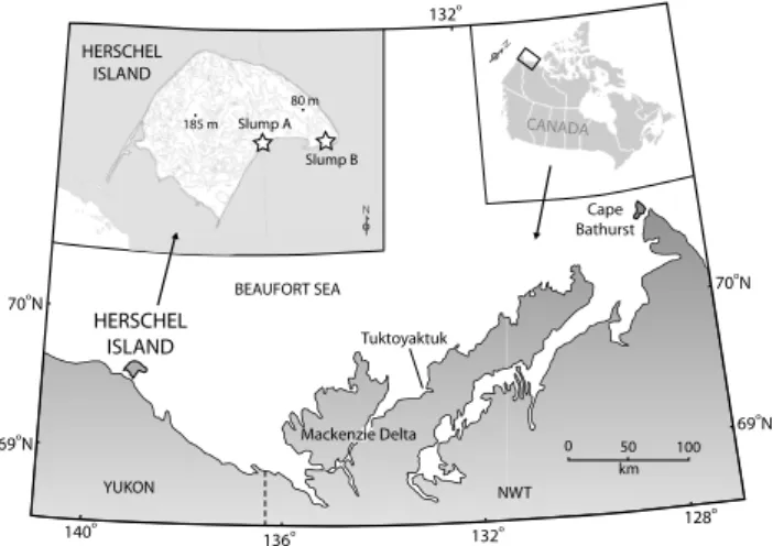
132o 70o N 69o N 128o 132o 136o 140o 69o N 70o N 0 50 100 km YUKON N N Slump A Slump B 185 m 80 m HERSCHEL ISLAND BEAUFORT SEA NWT Tuktoyaktuk Cape Bathurst Mackenzie Delta CANADA HERSCHEL ISLAND
Fig. 1. General study area is Herschel Island; the map inset displays the location of slumps A and B.
al., 2003). An increase in SOC released by Arctic coasts would potentially modify the carbon balance of the Arctic Ocean (Rachold et al., 2003). Under most climate change scenarios thermokarst processes are expected to increase, but since there are no long-term studies of thaw-related volume losses and only a few estimates of carbon content (Bockheim et al., 1999), this potential contribution is largely unknown (Lewkowicz, 1991). The recycling of carbon is a potentially important positive climate change feedback.
The prediction and analysis of retrogressive thaw slump activity remains difficult due to the variable nature of ground ice distribution (Pollard and French, 1980). Furthermore, their remote setting makes direct observation of this type of erosion and the analysis of potential climate feedbacks (like carbon fluxes) extremely problematic. Therefore, new tools and techniques are needed to monitor and predict the pro-gression of these landforms once they begin. Despite their potentially significant impact on arctic landscapes only a few studies have attempted to quantify the areas affected or the volumes of material eroded during retrogressive thaw slump occurrence (de Krom, 1990) and no study has used remote sensing to develop three-dimensional models to compute the magnitude of thaw or polycyclic retrogressive thaw slump development. This study uses stereophotogrammetric meth-ods to develop a three-dimensional geomorphic analysis of retrogressive thaw slumps that allows an estimation of the volume of sediment/ground ice eroded through back wasting thermokarst activity, and based on data from the Barrow area of Alaska, provides a first approximation of potential soil or-gan carbon released.
2 Objectives
Herschel Island is located on the Yukon coast between the Mackenzie Delta and Alaska in the southern Beaufort Sea (Fig. 1). This area is characterized by the largest and highest density of retrogressive thaw slumps in the Canadian Arctic
Fig. 2. Typical bowl-shaped retrogressive thaw slump in Thetis Bay, Herschel Island, July 1986.
(Lantuit and Pollard, in review1). In view of the significant
role played by thermokarst in the landscape evolution of this area, limited geodetic information, as well as its remote and inaccessible location, Herschel Island is an ideal site to test the applicability of remote sensing techniques in the analysis of thermokarst processes.
The goals of this paper are: (1) to demonstrate the value of stereophotogrammetric methods in mapping volume losses associated with two retrogressive thaw slumps on Herschel Island between 1952 and 2004, (2) to estimate the total vol-ume of sediment and ground ice eroded from these two retro-gressive thaw slumps during the same period, and (3) to map the morphological evolution of these features including their polycyclicity.
3 Background
The Yukon Coastal Plain and Mackenzie Delta are under-lain by continuous permafrost up to 600 m thick (Ramp-ton, 1982; Young and Judge, 1986). Permafrost is ground
that remains at or below 0◦C for a minimum of two years
(van Everdingen, 2002). However, in most areas of con-tinuous permafrost frozen conditions have existed for many 1000’s to 10 000’s years. Permafrost conditions in the west-ern Canadian Arctic reflect the complex pattwest-ern of glacial events during the Pleistocene and Holocene. Typically ar-eas of Pleistocene permafrost are much thicker than arar-eas of more recent permafrost aggradation (Rampton, 1982). The permafrost profile includes a thin surface layer that season-ally freezes and thaws called the active layer that is under-lain by a layer of seasonal temperature variation (∼10–15 m thick) beneath which equilibrium permafrost temperatures mirror the geothermal gradient. The nature and depth of per-mafrost is closely related to the mean annual ground surface temperature and the geothermal gradient (French, 1996).
Ground ice is a common constituent of permafrost
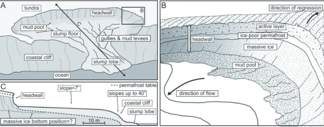
Fig. 3. Conceptual scheme of retrogressive thaw slump. Inset B focuses on the slump headwall. Inset C is a cross-section of the slump.
frozen moisture it varies greatly in character. If the volume of ice in the ground exceeds the total pore volume, the pro-portion in excess of saturation is termed “excess ice”. Upon thawing a soil containing excess ice consolidates releasing vast quantities of thawed water, termed supernatant water. Excess ice can occur in various forms, including segregated ice, buried glacier and snowbank ice, massive tabular ice and ice wedge ice (Mackay, 1972). The term massive ice refers to a body of ground ice with an ice content of at least 250% on an ice-to-dry-soil weight basis (Mackay, 1971). The degra-dation of massive ice leads to thermokarst.
Thermokarst is the process by which characteristic land-forms result from the thawing of ice-rich permafrost or the melting of massive ice (van Everdingen, 2002). The nature and magnitude of thermokarst is directly related to the ther-mal stability of the upper part of permafrost, including the depth of the active layer, and ground ice content. Two types of thermokarst are described in the literature, thermokarst subsidence and thermal erosion. Thermokarst subsidence is primarily vertical in direction and involves downwear-ing while thermal erosion involves lateral planation and is a backwasting process (French, 1996). Retrogressive thaw slumps are often polycyclic in nature. This refers to the for-mation of new retrogressive thaw slumps within the floor of an older retrogressive feature (Mackay, 1966; Wolfe et al., 2001). The older slump can be active or stable. The new retrogressive thaw slump will develop a similar shape to its parent. It is not uncommon to find several genera-tions of retrogressive thaw slumps within the same slump. Polycyclic retrogressive thaw slumps are readily identified using high-resolution airborne imagery (Lantuit and Pollard, in review1).
Retrogressive thaw slump headwalls are often hundreds of metres long and are occasionally as much as a kilome-tre. Retrogressive thaw slump morphology (Figs. 2 and 3) includes, (1) a vertical “headwall” that includes the active layer and a thin layer of ice-poor organic and mineral
materi-als, (2) a “headscarp” of a steeply inclined (20 to 50◦)
expo-sure of ice-rich sediment that retreats by ablation due to sen-sible heat fluxes and solar radiation, and (3) the slump floor, consisting of a mud pool at the base of the headscarp and a zone of saturated mud forming levees and flow deposits that expand in a lobate pattern at the toe of the slump (de Krom, 1990; Lewkowicz, 1987). Headwalls 10–20 m high retreat at rates that can average up to 9.6 m/yr for several years and as much as 30 m in exceptional year (de Krom, 1990; Lantuit et al., 2005). This magnitude of landscape change constitutes a potential hazard for both natural systems and engineered structures (Huscroft et al., 2003).
Retrogressive thaw slumps are initiated when erosion re-moves the layer of sediment that thermally protects ice-rich materials. For example, waves at the base of ice-rich coastal cliffs may expose a massive ice body leading to ice ablation and backwasting thermokarst (de Krom, 1990). If the ex-posed massive ice body thaw rate exceeds the rate of wave-induced erosion at the base of the cliff, then a retrogressive thaw slump is initiated and sustained (Lewkowicz, 1987). In some coastal locations, the frequency of retrogressive thaw slump activity is linked to the intensity of wave action and coastal processes. The removal of retrogressive thaw slump debris along the coast by wave action or littoral drift helps maintain a steep shore gradient. This facilitates the removal of sediment and prevents the build-up of debris at the base of the headwall or on the retrogressive thaw slump floor.
There is little information on SOC in permafrost soils.
Bockheim et al. (1999) found that SOC averaged 50 kg/m3
in the area around Barrow Alaska. In this study soils typical
of “Meadow Tundra” ranged from 24 to 109 kg/m3(average
48±23 kg/m3). About 47% of the SOC in the upper meter
of soil was in the active layer at the time of sampling; the remainder occurring in the permafrost. Some of the varia-tion in SOC was linked to differences the amount of ground ice. There is no information on SOC content from deeper in the permafrost profile but one could logically assume that it would be related to sediment history.
Slumps locations Study sites 185 m 80 m Avadlek Spit Osborn Point Thetis Bay Herschel Spit Collinson Head
Slump A
Slump B
3 kmHERSCHEL ISLAND
QIKIQTARUK
Fig. 4. Location of main retrogressive thaw slump activity and study sites on Herschel Island.
4 Study area
The primary focus of this study is Herschel Island (Fig. 1), a small island in the southern Beaufort Sea. Because of its historical significance to the Inuvialuit people, in 1990 Her-schel Island was set aside as a territorial park called Qik-iqtaruk. Herschel Island lies approximately 60 km east of the Yukon/Alaska border, 160 km west of the Mackenzie Delta and 3 km north of the continental coast. It is part of the Yukon Coastal Plain physiographic region, which is an eroded bedrock surface covered by marine, fluvial and glacial deposits. Herschel Island is a push moraine associated with late Pleistocene fluctuations of the Laurentide ice sheet (ca. 40 000 BP; Rampton, 1982).
Ice contents in the permafrost on Herschel Island are up to 20% higher than elsewhere on the Yukon Coastal Plain (Pol-lard, 1990). Ground ice underlies most of the island except under recent coastal landforms such as sand spits and sandy-pebbly beaches, and constitutes up to 60–70% (excess ice) of the upper 10–20 m of permafrost (Pollard, 1990). Mas-sive ice is widely observed on the island in coastal sections and active layer detachments on south, southeast and north-west facing shores (Fig. 4). The thickness of massive ice ranges between 4 and 20 m but is probably greater since only the upper part of the ice body is visible in coastal exposures (de Krom, 1990; Pollard, 1990). This part of the southern Beaufort Sea is not only one of the most ice-rich areas in the Canadian Arctic, but it is also an area of considerable hydro-carbon reserves and one of the more heavily populated areas. It is therefore likely that both community and resources in-frastructure will undergo increasing threat due to thermokarst activity.
4.1 Retrogressive thaw slump activity on Herschel Island
The retrogressive thaw slumps on Herschel Island are among the largest and most numerous encountered in the Canadian Arctic (de Krom, 1990). The rates of coastal erosion
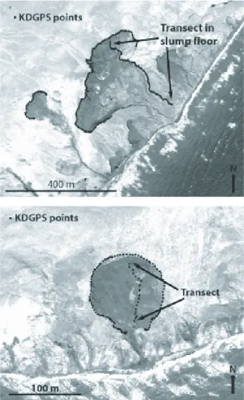
ob-Fig. 5. (a) 2004 Ikonos panchromatic view of slump A with KDGPS points surveyed two days later overlaid. (b)2004 Ikonos panchro-matic view of slump B with KDGPS points surveyed a day later overlaid.
served on the island range between 0.3 and 2 m/yr and con-tribute to the development of retrogressive thaw slumps. In addition, coastal erosion is often observed to increase fol-lowing the occurrence of thaw slumps (Lantuit and Pollard, in review1).
During the period from 1952 to 2000 retrogressive thaw slump frequency and area have increased on Herschel Island and are expected to continue to increase due to global
warm-ing (Lantuit and Pollard, in review1; Lewkowicz, 1991).
Fig-ures 5a and 5b show two retrogressive thaw slumps (Slump A and Slump B) in an area characterized by intense coastal
erosion (Lantuit and Pollard, in review1). Slump A is a
large polycyclic retrogressive thaw slump that has been ac-tive since at least 1952, while Slump B is a simple bowl-shaped retrogressive thaw slump which appears on post-1970 imagery. Slump A extends 600 m laterally while Slump B is roughly 150 m wide. Both slumps have massive ice bodies up to 20 m thick exposed in their headwalls.
5 Methods
The calculation of soil volume losses relies on the creation of three-dimensional surfaces or DEM’s (Digital Elevation Models) for each period. The creation of a high resolu-tion DEM is achieved using a combinaresolu-tion of geodetic sur-veys, high-resolution Differential Global Positioning Sys-tem (DGPS) surveys and stereophotogrammetric methods. While the first two provide a higher accuracy for three-dimensional measurements, they require extensive surface coverage. Stereophotogrammetric methods, although relying largely on the accuracy of ground control points, can be used to build three-dimensional surfaces over much larger areas. In remote locations like the Arctic, ground-based surveys cannot be completed with any regularity so stereophotogram-metric analyses are a possible alternative. In this study, soft-copy stereophotogrammetric tools are used to compile air-photos of Herschel Island for 1952 and 1970, and Ikonos panchromatic stereo-pairs for 2004.
5.1 Georeferencing controls for remotely sensed imagery
The first step in processing air photo and satellite imagery is to acquire a common georeferenced database. This is dif-ficult to achieve because there is little high quality geodetic data available for this part of the western Arctic and Herschel Island is both remote and difficult to access. Georeferenc-ing of digital images of Herschel Island was based on aero-triangulated coordinates from the 1970’s and 1:50 000 scale topographic maps. Topographic maps at scales of 1:50 000 and 1:250 000 are available for the entire southern Beau-fort region, but are not reliable enough for precise position-ing. Differences in a position derived from a topographic map and determined by sub metre GPS are often greater than 40 m. Published geodetic control points are more ac-curate but are limited along the Yukon Coastal Plain. Post-processed Kinematic Differential Global Positioning System (KDGPS) points were collected in September 2003 and Au-gust 2004 using a Trimble 4700 GPS system to provide accu-rate georeferencing. The horizontal and vertical accuracy of the outputs are within 2 cm when rigorously post processed. An error of this magnitude is negligible when compared with the expected accuracy of stereophotogrammetric analyses. A 0.5 m resolution was assumed when locating ground control points in photo space. The same stable landforms were iden-tified on the three sets of imagery in order to collect the GPS control points in the field. These points, referred to poly-gon edge intersections or artificial features, were all located inland and on stable slopes. The point location was docu-mented using field photography. Changes related to either thaw subsidence or isostatic adjustment were not considered because: (1) their magnitude is likely very small over this period and (2) there are insufficient long-term data to make these corrections. The points chosen are evenly distributed over the island. To assess the quality of the extracted DEM, a KDGPS survey of the slump headwalls and the slump floors
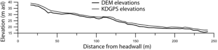
0 50 100 150 200 250 15 20 25 30 35 40
Fig. 6. Slump floor profile of slump A from KDGPS points and DEM. The x distances indicate the distance from the top edge of the headwall measured on the Ikonos imagery.
was completed on 8 August 2004, three days after the image was acquired by the Ikonos sensor.
5.2 Stereophotogrammetric processing of remotely sensed
imagery
Softcopy photogrammetric software was used to create the DEMs. Airphoto blocks were georeferenced according to the KDGPS survey points and DEMs were produced using the stereomatching algorithm of the softcopy software. The to-tal Root Mean Square (RMS) error for the 17 ground control points after bundle adjustment was 1.69 m for the 1952 im-age series, and 1.58 m for the 1970 imim-age series. The DEM spatial resolution was derived from the scanning resolution used for the airphotos. Airphotos from 1952 (28 August, 1:60 000) were scanned at 1600 dpi and produced an effec-tive resolution of 1 m while airphotos from 1970 (20 August, 1:13 000) were scanned at 800 dpi and produced an effective resolution of 0.3 m, later re-sampled to 1 m. The 2004 DEM was extracted from an Ikonos panchromatic stereo-pair (1 m resolution) acquired on 5 August 2004 using the method de-scribed by Toutin et al. (2001) and implemented in the soft-copy photogrammetric software. Resulting DEMs were then edited and a mosaic created to produce 1 m pixel ground res-olution DEMs of the area surrounding the retrogressive thaw slumps. The subtraction of both DEMs gave a GIS layer for differential volume erosion over the 1952–1970 and 1970– 2004 periods, respectively (Figs. 5a, 5b). Pixels correspond-ing to losses of sediment were aggregated and used to calcu-late volume erosion.
5.3 Accuracy assessment
The KDGPS points collected in the field three days after the acquisition of the Ikonos stereo-pair were used to assess the accuracy of the computed DEMs. The KDGPS points have an estimated accuracy of ±2 cm, which is sufficient for the type of accuracy typically associated with DEMs extracted from Ikonos stereo-pairs (Valadan and Toosi, 2003). Two transects of the floors of the retrogressive thaw slumps were conducted. Due to the pattern of mudflows present within the slumps floors, transects could not be performed along per-fectly straight lines (Fig. 5a, 5b) although they were kept as straight as possible. Once processed in the softcopy pho-togrammetric software, the DEMs were overlaid and com-pared to the KDGPS points. The resulting profiles are shown in Figs. 6 and 7, respectively. The DEMs computed for the
0 20 40 60 80 100 24
28 32 36
Fig. 7. Slump floor profile of slump B from KDGPS points and DEM. The x distances indicate the distance from the top edge of the headwall measured on the Ikonos imagery.
years 1952 and 1970 were controlled using KDGPS points collected during the summer of 2004. These check-points were located on ice wedge trough edges or closed thaw ponds chosen for their stability between 1952 and 2004. Volume losses associated with retrogressive thaw slump oc-currence were computed for the 1952–1970 and 1970–2004 periods for slump A and the 1970–2004 period for slump B. On slump A measurements were performed on a 600 m section of coast extending 200 m inland, excluding volume losses associated with coastal erosion. On slump B, volume losses were estimated on a 100 m long strip of coast extend-ing 100 m inland.
5.4 Sediment erosion
In order to assess the amount of sediment eroded from the slumps that is then transported into the nearshore zone, it is necessary to consider any bias in the calculations from the large quantities of ground ice associated with retrogressive thaw slumps. Typically, massive ice bodies in retrogressive thaw slump headwalls are exposed from the base of the over-burden to the slump floor. The overover-burden consists of the active layer and a metre of ice-poor material. Its lower limit is associated with the hypsithermal thaw unconformity ob-served elsewhere in the area by Harry et al. (1988). The lower part of the massive ice section is generally concealed by mud that pools at the base of the headwall. The volumetric ice content of these massive ice bodies is up to 90% on Herschel Island (Pollard, 1990). The resulting proportion of sediment in these bodies can therefore be estimated to be 10% of to-tal volume extending below the active layer. Observed ac-tive layer depths ranges from 15 to 90 cm comparable with data in Kokelj et al. (2002), depending on the sampling site. Undisturbed tundra surfaces are generally characterized by a shallow active layer up to 45 cm thick, while the active layer in thaw consolidated sediments in stabilized slump floors are up to 90 cm. Since Slump A and Slump B occur in former slumps we assumed a constant active layer depth of 90 cm (Lantuit and Pollard, in review1).
A perennially frozen layer of ice-bonded sediment with negligible excess ice content underlies the active layer and unconformably overlies the massive ice (Pollard, 1990). The layer of sediment that overlies the massive ice can therefore be considered free of excess ice and was assigned a volumet-ric ice content of 0%. Observations in the field on 8, 9 and
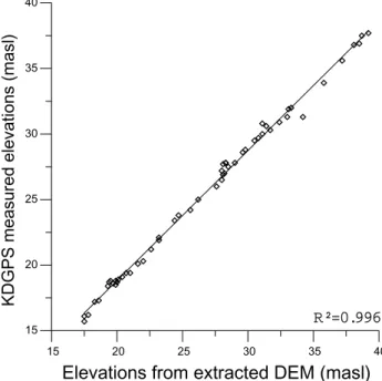
15 20 25 30 35 40 15 20 25 30 35 40 R²=0.996
KDGPS measured elevations (masl)
Elevations from extracted DEM (masl)
Fig. 8. Scatter plot of KDGPS versus DEM elevations along the transect in slump A. Best least squares fit regression line is super-imposed.
10 August 2004 showed that the total thickness of this layer of overburden was on average 1.5 m.
The total volume of sediment enclosed within the ice and released to the nearshore zone through the slumping process was estimated using Eq. (1),
V sice =
n
X
i=1
[Ai · (1hi − Zo) (1 − θ )] , (1)
where V sice is the total volume of eroded sediment from the
ice (m3) through the slumping process, Ai is the area (m2)
of the pixel, 1hi the computed difference (m) of elevation between the DEMs, Zo is the mean overburden depth (m), θ the volumetric ice content (%) for massive ice bodies and n the total number of pixels considered in the calculation.
In addition, the total volume of sediment eroded from the overburden was calculated using Eq. (2),
V so =
n
X
i=1
(Ai · Zo) , (2)
where V so is the total volume of sediment eroded from the overburden through the slumping process. The addition of Eqs. (1) and (2) provide an estimate of the total volume of sediment eroded from the slump (V s) as noted in Eq. (3). Equation (3) was solved using a Geographic Information System (GIS) to estimate the resulting sediment volumes for both slumps.
V s =
n
X
i=1
Table 1. Eroded sediment volumes from retrogressive thaw slumps A and B.
Volumes for slump A (m3) Volumes for slump B (m3)
1952–1970
Total volume loss 585 900 none
Total eroded sediment volume 104 300 none
Eroded sediment from overburden 51 100 none
Eroded sediment from massive ice 53 200 none
1970–2004
Total volume loss 1 566 900 105 900
Total eroded sediment volume 355 000 22 300
Eroded sediment from overburden 222 200 13 000
Eroded sediment from massive ice 132 700 9200
6 Results
6.1 Accuracy assessment
The elevations extracted from the Ikonos stereo-pair and the airphotos need to be consistent with KDGPS elevations to provide accurate measurements of volume losses.
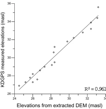
The elevations obtained from the 2004 DEM along tran-sect locations within the two slump floors were consistently lower than the KDGPS profiles by an average of 1.2 m in slump A and 1.7 m in Slump B. Single deviations never ex-ceeded 3 m, and in the case of Slump A were within 2 m 98% of the time. Overall, the shapes of the profile were quite similar. A simple regression analysis between KDGPS and DEM elevations run for the two slumps (Figs. 8 and 9) show a strong correlation for both slumps (0.996 for Slump A and 0.961 for Slump B) and regression slopes of 1.02 and 0.94, respectively. The elevations extracted from the 1952 and 1970 DEMs were observed to be within 1.2 m of the checkpoint elevations. A stable checkpoint located 50 m in-land from the slump headwall in 2004 showed a deviation of 0.9 m with the 1952 DEM and of 1.1 m for the 1970 DEM. The latter deviations corresponded to an underestimation of the elevations by the DEM stereo-matching algorithm. Given the consistent (<1 m) underestimation of elevations by the DEM algorithm throughout the study period, we chose to use uncorrected raw values for volume calculations.
6.2 Eroded sediment volumes
Eroded sediment volumes are presented in Table 1 and for this study are basically assumed to equal the volume of the depression produced by the retrogressive thaw slump. Re-sults are summarized by period and type of volume loss (i.e. total volume loss, total eroded sediment and ice, eroded sed-iment from the overburden, eroded sedsed-iment from massive ice). Since Slump B started after 1970, no values are pre-sented for the 1952–1970 period. Volume losses for the two slumps varied greatly. While Slump B can be considered a “small” slump in comparison with others on the island, Slump A is a large slump marked by considerable sediment and ice volume loss. Volume losses in Slump A increased by
R² = 0.961
24 26 28 30 32 34 26 28 30 32 34 36KDGPS measured elevations (masl)
Elevations from extracted DEM (masl)
Fig. 9. Scatter plot of KDGPS versus DEM elevations along the transect in slump B. Best least squares fit regression line is super-imposed.
300% (585 900 m3to 1 566 900 m3) between the 1952–1970
and the 1970–2004 periods. In addition, the difference in volume of eroded sediment between Slump A and Slump B
differed by a factor of 16 (355 000 m3vs. 22 200 m3,
respec-tively).
The volume of sediment eroded from the overburden was always greater than or similar to that eroded from the mas-sive ice layer. For example, in the case of Slump A during
the period 1970–2004 222 300 m3(63%) of sediment is
de-rived from the overburden while 132 700 m3(37%) is from
massive ice. Of the total volume of sediment eroded roughly 51% was derived from the overburden and 49% from massive ice during the 1952–1970 period. In the case of Slump B, which is expanding in a typical bowl-shaped fashion, volume of sediment eroded from massive ice accounted for roughly 42% of the total sediment loss.
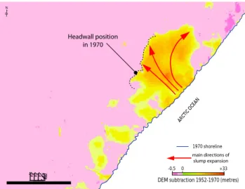
200 m DEM subtraction 1952-1970 (metres)
-0.5 0 +33 1970 shoreline
ARCTIC OCEAN
Fig. 10. Volume losses map for 1952–1970 in slump A. Losses are associated with the vertical difference between the 1970 and 1952 DEMs. Note the presence of discrete spots of greatest erosional values within the slump floor, probably pinpointing the occurrence of two stages of slump activity (polycyclicity).
200 m
DEM subtraction 1970-2004 (metres)
-0.5 0 +33 2004 shoreline
ARCTIC OCEAN
Fig. 11. Volume losses map for 1970–2004 in slump A. Losses are associated with the vertical difference between the 2004 and 1970 DEMs. Note the location of the greatest erosion immediately below the current headwall. The more littoral part of the slump is characterized by the presence of stable zones (pink) and zones currently eroding (greenish colors).
6.3 Mapping thermokarst volumes
The spatial pattern of retrogressive thaw slump formation is illustrated in Figs. 10, 11 and 12. Slump A expands along an east-west axis but retains the same shape. The main zone of erosion during both periods is in the centre of the main headwall. Exposures along the sides generally display low rates of erosion; this pattern tends to accentuate the higher losses from the centre of the headwall. This pattern is
il-100 m
DEM subtraction 1970-2004 (metres)
-0.5 0 +33 2004 shoreline
Fig. 12. Volume losses map for 1970–2004 in slump B. Losses are associated with the vertical difference between the 2004 and 1970 DEMs. Arrows indicate the direction of slump expansion. Note the constant width of the slump and the fairly homogeneous values for DEM subtraction. These indicate the likely presence of a continuous massive lens which was melted in a headwall of constant height.
lustrated best by comparing losses from the 1970–2004 with those from 1952–1970. The main zone of erosion (where vertical difference 1hi exceeds 15 m) has tripled in size be-tween the two periods. In Slump B, the greatest zone of ero-sion is also in the middle of the headwall. However, because of the small size of Slump B differences in vertical variations are not as obvious as Slump A.
7 Discussion
7.1 Sediment supply to the nearshore zone
In most coastal studies concerned with sediment fluxes in the coastal zone, erosion rates are usually related to storm and related wave activity. However, this study clearly demon-strates the potential significance of thermokarst as a sediment supply process along ice-rich permafrost coasts. The large differences in volume loss estimated for slumps A and B also demonstrate the variable nature in both ground ice con-tent and rate of thermokarst over relatively short distances. For these reasons any study concerned with rates and vol-umes of erosion or thermokarst needs to focus on individ-ual features with a particular emphasis on the shape and size of retrogressive thaw slumps. The occurrence of retrogres-sive thaw slumps and the flow of liquefied mud can sup-ply large amounts of sediment to the nearshore zone and in some cases more sediment than coastal erosion. For ex-ample, Lantuit (2004) computed an average coastal erosion rate of 1 m/yr for this part of Herschel Island. Therefore in the case of Slump A, 1 m/yr erosion on a 20 m high coastal bluff over a 600 m length of shoreline for the period 1970–
2004 would result in a loss of roughly 420 000 m3 of
sed-iment and ice. With excess ice contents up to 60% along
sediment and 259 400 m3of ice were eroded. By compar-ison, thermokarst processes associated with Slump A yield
approximately 355 000 m3 of sediment which is
consider-ably greater than cliff erosion. Similarly for Slump B, the sediment volume removed by coastal erosion is estimated
at 51 000 m3 for the 1970–2004 period, with an additional
22 246 m3of eroded sediment from the slump itself.
7.2 Soil organic carbon
Bockheim et al. (1999) found that the SOC content
in “Meadow Tundra” near Barrow, Alaska averaged
48±23 kg/m3. Since Herschel Island is characterized by
pre-dominantly Meadow Tundra and given its close proximity to Barrow and similarities in climate and vegetation cover, it is likely to have similar SOC contents. However, Bockheim et al. (1999) focused on the top 1–2 m of permafrost where SOC contents are likely to be greatest due to recent organic depo-sition and biological processes. It is unlikely that these SOC contents exist to the depths thawed on Herschel Island. Given that Herschel Island is composed of glacially thrust marine and coastal sediments, it is not unrealistic to expect mod-erate amounts of SOC to exist through the depths disrupted by thermokarst. Assuming that the permafrost sediments of Herschel Island have similar values of SOC for the upper 2 m and conservative levels through the rest of the eroded sed-iments, it is assumed that SOC contents are approximately
10–25 kg/m3. If Slump A contributes 355 000 m3 of
sedi-ment to the nearshore zone through thermokarst then the
po-tential SOC contribution is roughly 3.5–8.9×10⁶kg.
Sim-ilarly the 22 246 m3of sediment eroded from Slump B
in-cludes potentially 2.2–5.6×10⁵kg of SOC.
7.3 Retrogressive thaw slump polycyclicity
Slump B’s headwall retreat is mainly normal to the coast with little expansion parallel to the coastline, whereas in Slump A the migration of the headwall is both landward and parallel to the coastline. The complex pattern of erosion for Slump A is a reflection of its large size, rapid retreat of its headwall and the reactivation of thermokarst in the slump floor. Erosion for the 1970–2004 period (Fig. 11) clearly shows volume losses from the older part of the slump (exposed during the 1952– 1970 period) as well as the headwall. Erosion of older slump surfaces reflects the development of small polycyclic slumps in the floor of Slump A. Polycyclic behaviour is the result of the incomplete melting of massive ice that typically occurs during headwall retreat (Mackay, 1966). The accumulation of sediment at the base of the headwall protects the lower part of the ground ice exposure from melting and progressively reduces the amount of ice exposed. As the headwall retreats a portion of the massive ice body is buried under the slump floor (de Krom, 1990). In theory the thickness of exposed massive ice in the retreating headwall decreases at a rate pro-portional to the thickness of the overburden times a flowage factor. The migration of the headwall and the accumulation of sediment and water on the slump floor form pools of
lique-fied mud that flow down slope in channels 2–3 m wide toward the coast. The efficiency of this process (flowage) determines how much sediment remains at the base of the headwall, how much pools near the headwall and how much sediment flows into the ocean. It also determines the thickness of sediment covering ground ice in the floor of the slump and therefore the thermal stability of the buried ground ice. It often takes 5-10 years for the floor of a slump of dimensions of 100 m and more from the headwall to stabilize.
Water and liquefied mud flowing across the stable slump floor gradually erode a network of channels and gullies (see Figs. 5a and 5b). Where massive ice in the slump floor is exhumed by gully erosion a new retrogressive thaw slump may be initiated. By using DEMs to map erosion patterns in retrogressive thaw slumps it is possible to differentiate both reactivated thermokarst and stable surfaces likely to be reac-tivated. The stable areas of the floor of Slump A on Fig. 11 (i.e. older parts of the slump floor) are the most likely loca-tions of future retrogressive thaw slump activity.
As mentioned previously, slumps A and B developed within the limits of former retrogressive thaw slumps that had been stable for over 50 years (Lantuit and Pollard, in
review1), which means that the current study is concerned
with a second generation of slump occurrence. Since no vol-ume loss is measured in the zones located above the head-walls prior to 1952, it appears that residual massive ice bod-ies up to 20 m can be concealed during long periods of slump inactivity.
8 Conclusions
This study includes possibly the first long-term calculations of sediment and ground ice volume losses associated with retrogressive thaw slump activity. It is also the first study to use remotely sensed data to determine the rates of retreat and volume losses based on sequential DEMs. Since retrogres-sive thaw slump frequency appears to be increasing on Her-schel Island and across the Arctic, total volume losses asso-ciated with these major thermokarst landforms are expected to increase through the 21st century. The DEMs extracted using stereophotogrammetric methods show that the volume of sediment eroded from retrogressive thaw slumps on arctic coasts is significant and of the same order of magnitude as coastal erosion. Given the recent emphasis on estimates of eroded sediment and carbon from arctic coasts to the Arctic Ocean (Rachold et al., 2003), it seems appropriate to con-sider the role of retrogressive thaw slumps and ultimately of ground ice in these calculations. Calculations from Herschel Island show that along a 600 m section of coast, retrogres-sive thaw slump-related eroded sediment is approximately
355 000 m3 which is greater than the 180 600 m3 expected
to be supplied by coastal cliff erosion alone. The estimated
SOC associated with these sediments is 3.5–8.9×10⁶kg.
This study also demonstrates that stereophotogrammetric methods are a useful tool to determine the long-term dynam-ics within thermokarst areas and based on a series of simple
assumptions provide a way of identifying areas of potential polycyclic reactivation. The high costs associated with high-resolution satellite imagery can be seen as a deterrent for the use of such methods to investigate landscape dynamics, how-ever, in comparison with the high cost of field research in re-mote areas like the Canadian Arctic this approach provides a realistic alternative. The expected increased frequency of ret-rogressive thaw slump activity associated with global warm-ing represents an imminent threat to arctic communities lo-cated in ice-rich regions such as the western Canadian Arctic. In this sense, stereophotogrammetric tools can serve as pow-erful monitoring tools to detect retrogressive thaw slumps.
Acknowledgements. This research was supported by the Natural
Science and Engineering Research Council of Canada (W. Pollard). Support from the Polar Continental Shelf Project (PCSP) and the Aurora Research Institute (ARI) for the field component was greatly appreciated. H. Lantuit is supported by the Warren fellow-ship in GIS, McGill University and the Government of Canada Award Program administered by the International Council for Canadian Studies (ICCS) on behalf of the Department of Foreign Affairs and International Trade of Canada (DFAIT). The imagery is generously provided by the McGill Electronic Data Resources Service (EDRS). The field assistance of N. Couture, J. Turner and T. Haltigin is gratefully acknowledged. The authors wish to express sincere appreciation to the Yukon Territorial Government, to the Yukon Parks, Yukon Department of Renewable Resources and to the Environmental Impact Screening Committee (EISC), and to the Inuvialuit Renewable Resource Committees for their support and encouragement of this project. The authors also wish to thank C. Davey from McGill University and A. Blais-Stevens and another referee for their helpful comments on this paper.
Edited by: M. Jaboyedoff
Reviewed by: A. Blais-Stevens and another referee
References
Bockheim, J. G., Everett, L. R., Hinkel, K. M., Nelson, F. E., and Brown, J.: Soil organic carbon storage and distribution in arctic soils, Barrow, Alaska. Soil Sci. Soc. Am. J., 63, 934–940, 1999. de Krom, V.: Retrogressive thaw slumps and active layer slides on Herschel Island, Yukon., M.Sc. Thesis, McGill University, Montr´eal, Qu´ebec, 157, 1990.
French, H. M.: The Periglacial Environment (2nd edition), Addison Wesley, Longman Limited, Harlow, UK, 341, 1996.
Harry, D. G., French, H. M., and Pollard, W. H.: Massive ground ice and ice-cored terrain near Sabine Point, Yukon coastal plain, Can. J. Earth., 25, 1846–1856, 1988.
Huscroft, C. A., Lipovsky, P., and Bond, J. D.: Permafrost and land-slide activity: Case studies from southwestern Yukon Territory, In: Yukon Exploration and Geology 2003, edited by: Emond, D. S., and Lewis, L. L., Yukon Geological Survey, 107–119, 2003. Kokelj, S. V., Smith, S. A. S., and Burn, C. R.: Physical and
chem-ical characteristics of the active layer and permafrost, Herschel Island, Western arctic Coast, Canada, Permafrost and Periglacial Processes, 13, 171–185, 2002.
Lantuit, H.: Fifty years of coastal erosion and retrogressive thaw slump activity on Herschel Island, Southern Beaufort Sea, Yukon
Territory, In: Mapping ground-ice related coastal erosion on Her-schel Island, Southern Beaufort Sea, Yukon Territory, Canada., M.Sc. Thesis, McGill University, Montr´eal, Quebec, 135, 2004. Lantuit, H., Couture, N., Pollard, W. H., Haltigin, T., De Pascale,
G., and Budkewitsch, P.: Short-term evolution of coastal poly-cyclic retrogressive thaw slumps on Herschel Island, Yukon Ter-ritory, Berichte zur Polarforschung, in press, 2005.
Lewkowicz, A.G.: Headwall retreat of ground-ice slumps, Banks Island, Northwest Territories, Can. J. Earth., 24, 1077–1085, 1987.
Lewkowicz, A. G.: Climatic Change and the Permafrost Land-scape., in: Arctic environment: Past, Present and Future, edited by: Woo, M. K. and Gregor, D. J., Proceedings of a symposium, 14–15 November 1991, Department of Geography, McMaster University, Hamilton, 91–104, 1991.
Mackay, J. R.: Segregated epigenetic ice and slumps in permafrost, Mackenzie Delta, N. W. T., Geographical Bulletin, 8, 59–80, 1966.
Mackay, J. R.: The origin of massive icy beds in permafrost, west-ern arctic coast, Canada, Can. J. Earth., 8, 397–422, 1971. Mackay, J. R.: The World of Underground Ice, Annals Am. Assoc.
Geographers, 62, 1–22, 1972.
McGillivray, D. G., Agnew, T. A., McKay, G. A., Pilkington, G. R., and Hill, M. C.: Impacts of climatic change on the Beau-fort sea-ice regime: Implications for the arctic petroleum indus-try, Climate Change Digest CCD 93–01, Environnement Canada, Downsview, Ontario, 36, 1993.
Oechel, W. C., Vourlitis, G. L., Hastings, S. J., and Bochkarev, S. A.: Change in arctic CO2 flux over two decades: Effects of cli-mate change at Barrow, Alaska. Ecol. Applic., 5, 846–855, 1995. Pollard, W. H.: The nature and origin of ground ice in the Herschel Island area, Yukon Territory. Proc., Fifth Canadian Permafrost Conference, Qu´ebec, 23–30, 1990.
Pollard, W. H. and French, H. M.: A first approximation of the volume of ground ice, Richards Island, Pleistocene Mackenzie Delta, N. W. T., Can. Geotech., 17, 509–516, 1980.
Rachold, V., Eicken, H., Gordeev, V. V., Grigoriev, M. N., Hub-berten, H.-W., Lisitzin, A. P., Shevchenko, V. P., and Schirrmeis-ter, L.: Modern terrigenous organic carbon input to the arctic Ocean, in: Organic Carbon Cycle in the Arctic Ocean: Present and Past, edited by: Stein, R. and Macdonald, R. W., Springer Verlag, Berlin, 33–55, 2003.
Rampton, V. N.: Quaternary Geology of the Yukon Coastal Plain, Geological Survey of Canada Bulletin, 317, 49, 1982.
Serreze, M. C., Walsh, J. E., Chapin III, F. S., Osterkamp, T. E., Dyurgerov, M., Romanovsky, V. E., Oechel, W. C., Morison, J., Zhang, T., and Barry, R. G.: Observational evidence of re-cent change in the northern high-latitude environment, Climate Change, 46, 159–207, 2000.
Toutin, T., Chenier, R., and Carbonneau, Y.: 3D geometric mod-elling of Ikonos GEO images, Proc. Joint ISPRS Workshop on “High Resolution Mapping from Space 2001”, Hannover, 19– 21 September, Institute of Photogrammetry & Geoinformation, University of Hannover, 9 (on CD ROM), 2001.
Valadan Z. and Toosi, K. N.: Rigorous and non-rigorous pho-togrammetric processing of IKONOS-1 geo image, Proc. Joint ISPRS Workshop on ”High resolution mapping from space 2003”, October 2003, Hannover, Germany, 6 (on CD-ROM), 2003.
van Everdingen, R. O.: Multi-language glossary of permafrost and related ground-ice terms, Boulder, CO: National Snow and Ice Data Center/World Data Center for Glaciology, 200, 2002.
Wolfe, S. A., Kotler, E., and Dallimore, S. R.: Surficial charac-teristics and the distribution of thaw landforms (1970 to 1999), Shingle Point to Kay Point, Yukon Territory, Geological Survey of Canada, Open File 4088, 2001.
Young, S. and Judge, A. S.: Canadian permafrost distribution and thickness data collection: a discussion, in: Proceedings on National Student Conference on Northern Studies, edited by: Adams, W. P. and Johnson, P. G., 223–228, 1986.