HAL Id: hal-03028157
https://hal.archives-ouvertes.fr/hal-03028157
Preprint submitted on 11 Dec 2020HAL is a multi-disciplinary open access archive for the deposit and dissemination of sci-entific research documents, whether they are pub-lished or not. The documents may come from teaching and research institutions in France or abroad, or from public or private research centers.
L’archive ouverte pluridisciplinaire HAL, est destinée au dépôt et à la diffusion de documents scientifiques de niveau recherche, publiés ou non, émanant des établissements d’enseignement et de recherche français ou étrangers, des laboratoires publics ou privés.
constant?
Georges Poupinet
To cite this version:
Ray tracing on the sphere …and the fine structure constant?
G. Poupinet
Pa
P
a) ex CNRS scientist, ISTerre, Université Grenoble-Alpes, Grenoble, France
Marcel Duchamp, 1913; Roue de bicyclette, Réunion des Musées Nationaux
Résumé
La constante de la structure fine α (≈ 1/137), initialement introduite dans l’atome de Bohr, intervient dans le calcul de la force électromagnétique entre deux charges élémentaires. Cette constante sans dimension a été considérée comme une énigme importante en physique. En physique des particules, de nombreux calculs sont des sommes de termes en αn. Peut-on calculer une courbe dans l’espace reflétant ce nombre ? En procédant à des rotations dans deux plans orthogonaux, je calcule une courbe géométrique simple qui couvre la sphère. Cette clelia est une courbe de Viviani qui tourne autour de l’axe vertical. Pour une différence des vitesses de rotation liée à la meilleure approximation du nombre π par une fraction rationnelle, la longueur de la clelia (112,113) est de 137.028. L’application d’une inclinaison sinusoïdale de l’axe vertical d’amplitude (π/226) 2
donne une longueur de 137.035 999 3 (x 2 π) à cette
courbe, soit 9 chiffres identiques aux valeurs expérimentales de α-1. Ce calcul géométrique illustré ici à l’aide de la roue de bicyclette de Duchamp peut-il avoir un rapport avec la physique de base?
Abstract
The fine structure constant α (≈ 1/137), first introduced in Bohr’s model of the atom, intervenes in the calculation of the electromagnetic force between two elementary charges. This dimensionless constant has been considered an important enigma in physics. In particle physics, many computations are a sum of terms in αn . Can we calculate a three-dimensional curve reflecting this number? By carrying out infinitesimal rotations in two orthogonal planes, I calculate a simple geometric curve which covers the sphere. This clelia is a Viviani curve that rotates around the vertical axis. For a difference in rotation speeds related to the best approximation of the number
π by a rational fraction, the clelia (112,113) has a length of 2 π x 137.028. Applying a
sinusoidal tilt to the vertical axis of amplitude (π / 226) 2 gives a length of 137.035 999 3 (x 2 π) to this curve, i-e 9 digits identical to the experimental values of α-1. Is this
geometrical computation illustrated here by Duchamp’s bicycle wheel connected to basic physics.
Introduction
In his planetary model of the atom, Bohr (1913) found that v, the velocity of the electron around its circular orbit, is proportional to c, the velocity of light in the vacuum: in the CGS unit system, α = v/c = e2/ћc, where e is the charge of the electron and ћ is the Planck constant divided by 2π. Sommerfeld (1916) incorporated relativity in Bohr’s model and coined the term “fine structure constant” for the dimensionless quantity α. Since it was first introduced α has fascinated famous physicists such as Eddington, Dirac, Heisenberg, Pauli, Feynman, and many others. α-1, its inverse value, close to 137.035999, intervenes in the computation of the strength of the electromagnetic interaction between two electric charges, hence the qualifier of “electromagnetic” sometimes braced to α’s usual denomination. In quantum electrodynamics (QED), developments in αn are summed to compute the probability of
occurrence of particles. After Dirac introduced equations that describe the atom of hydrogen with a much better precision than Bohr’s model, Schrödinger (1930) found that solutions of the Dirac equations imply a ‘trembling motion’ of the atom of hydrogen. This so-called zitterbewegung can be thought of as a tiny precession-nutation, a concept which will reveal all its importance in the course of this article.
α-1
has also been a favorite subject of numerologists who found relationships between α-1
and natural numbers, some of them simple. Wilczek (1999), taking into consideration the Standard Model, however contests the primary role attributed to α-1 by Wolfgang Pauli: ‘The original idea of Pauli and others that calculating the fine
structure constant was the next great item on the agenda of theoretical physics now seems misguided. We see this constant as just another running coupling, neither more nor less fundamental than many other parameters, and not likely to be the most accessible theoretically’. Astronomers have recently revived the interest in α by
performing tests on its temporal stability (see Uzan, 2003). Kragh (2003) explains the important role of α in physics in a thorough historical review.
If the value of α cannot be deduced from any physical theory up to now, it can be measured from spectroscopic experiments with a remarkable precision. α-1 is given as 137. 035 999 074(44) by NIST in 2010. Gabrielse et al. (2006) and Kinoshita (2006) found a very precise value of 137. 035 999 710±0.000 000 096. This value was obtained after more than 800 terms of QED corrections. These QED corrections are tedious and errors were found in the initial corrections; so α-1 was later revised to 137.035 999 074, the value retained by NIST. In fact, the value of α-1
is also dependent on the measurement technique. In a measurement of α-1 using h/mRb, Cadoret et al (2008) find
α-1
= 137.035 999 45(62).
The sphere is a simple 3D object in geometry and spherical fields are widespread in physics. Bohr’s introduction of α as the ratio of two velocities, v and c, is also a clue to find some kind of trajectory as advocated by several physicists as for instance De Broglie. A sphere seems more appropriate than a circle for a computation inspired by the hydrogen atom. This paper is an attempt to relate α to a geometric curve on the sphere?
A singular curve on the sphere: Viviani’s curve
Viviani’s curve is the intersection of a sphere of radius r with a cylinder of radius r/2 positioned on one radius of the sphere. It is also ‘a portion of the section of the Möbius
surface by a sphere’ (Fig. 1; Ferréol). It was discovered in 1692 by Vincenzo Viviani
who was the last assistant of Galileo and by others like Roberval. For r=1, its parametric representation is: λ=φ (avoiding the modulo) or{x=sin φ cos φ, y=cos φ cos φ, z=sin φ }. On a sphere, Viviani’s curve is such that longitude φ equals latitude λ. From a practical point of view, Viviani’s curve is generated by two orthogonal rotations: a rotation φ in a meridian plane which itself rotates by φ around the vertical axis. It can be illustrated by Marcel Duchamp’s ‘roue de bicyclette’; a bicycle wheel is fixed to a fork (fig. 1). Both the fork (or handlebar) and the wheel rotate independently. We could attach small electric motors to the fork and to the axle of the wheel and fix a LED anywhere on the wheel. If both the fork (or handlebar) and the wheel rotate at the same speed, the LED describes a Viviani’s curve in the 3D space (Fig. 2). This trajectory is a kind of compromise between the sphere and the cylinder.
A unitary Viviani’s curve projects as a circle of radius 1/2 on the horizontal plane and as a circle of radius 1 on the rotating meridian plane. By analogy with what happens when a seismic ray is followed from the source to a given receptor, let us move on a Viviani’s curve by steps of ∂φ. We stop moving when the distance to the starting point is minimal,
without limiting the number of turns. Surprisingly, we always find the minimum distance after 113 complete turns, whatever ∂φ. The propagation length is always 137.4 x 2π. The
length of a Viviani’s curve is an elliptic integral equal to 7.64 (Ferréol) and 137.4 x 2π =
113 x 7.64, as found before. Why the number 113?
Fig. 2: Viviani’s curve from http://www.cfm.brown.edu , Matlab Tutorial
Let us approximate π by a fraction of integers. A well-known approximation is
π 22/7=3.14285. Around 500 AD, Zu Chongzhi found π 355/113 = 3.14159292, i-e π - 355/113 = 0.0000002667. The next best approximation is 52163/16604 with a residual of 0.0000002662, followed by 104348/33215 with a residual of 0.000000000332.
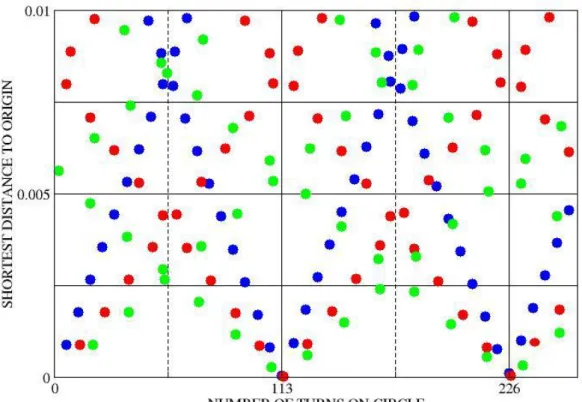
Let us construct a circle by adding iteratively a vector of a fixed length that rotates by a fixed angle at each step. The angle corresponds to the circle’s curvature. Starting from the origin, we propagate along a polygon whose vertices are on the circle. After several iterations, the trajectory returns near the origin. How many turns are necessary to return closest to the origin? It is always after 113 turns and multiples of 113, whatever the size of the generating vector (Fig. 3).
Figure 3: Construction of a circle by propagating iteratively a vector (colors correspond to different lengths). 113 turns are necessary to return near the origin whatever the length of the generating vector.
The clelia of argument (112,113) covering the sphere
To cover the entire sphere, we slowly rotate a Viviani’s curve around the vertical axis and this creates a clelia. Clelia were introduced by Grandi in 1728 (Ferréol). Returning to Duchamp’s ‘roue de bicyclettte’, when the two electric motors rotate at a different speed, the LED draws a clelia in 3D-space. The difference in the rate of the two rotations determines the density of the net covering the sphere. Let us consider the clelia whose parametric representation is φ = 112 x λ / 113 or
{x=sin(112 xλ / 113) cos(λ), y=cos(112 x λ / 113) cos(λ), z=sin(λ)}.
This curve returns to its origin after 113 complete quasi Viviani’s cycles. Latitude varies from 0 to 226 π and longitude varies from 0 to 224 π. For the bicycle wheel, the wheel axle’s motor should rotate slightly faster than the fork’s motor: the speed ratio being 112/113. The total length of the clelia of argument (112,113) is 137.028 x 2π. This clelia
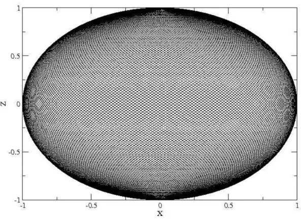
projects on the horizontal plane as a quasi-epicycloïd. The projection of the (112,113) clelia on a vertical plane is plotted on figure 4. This is also the path followed by the LED attached to the wheel as seen sideways.
Fig. 4: Clelia of argument (112,113) covering the sphere. The sphere is transparent and we visualize both sides; projecting on the x or y axis planes give different coverage of rays. The length of this curve is 137.028 x 2π.
Introducing a tilt of the meridian plane as zitterbewegung
This value of 137.028 is not exactly the experimental value of α-1, 137.035999. If the curve we are searching has some relationship with an electron, it should exhibit a kind of
zitterbewegung, which can be modeled as a trembling tilt of the meridian plane. If we
introduce new variables, various corrections could give the right value of α. Instead, we search for the simplest correction and avoid the use of new variable. We introduce a precession-nutation of the vertical axis of the clelia. Surprisingly, a correction by the very small angle - (π / 226) 2x (1. + cos(2 φ)) = - 2.0 x (π cos(φ) / 226) 2 gives an unexpected
result. From a geometrical point of view, this tiny correction projects as an ‘quasi-epicycloid’ on the horizontal plane; the z axis of the clelia is rotating at twice the speed of the main rotation around a precession axis. The precession circle has a radius (π / 226) 2 and rotates by π / 226 during each main ‘quasi Viviani’ cycle. This computation is listed in a Fortran program below. The result of this computation is α-1 = 137.035 999 3 for n = 100 000, the number of steps. The last digit becomes 4 for n 00 000.
Fortran program:
Using ray tracing inspired by seismology and optics, a spherical curve derived from Viviani’s curve, a clelia (112,113) (related to the approximation of π by 355/113) has a length close to α-1 (x 2π). In order to include a trembling motion, the zitterbewegung,
(proved by Schrödinger to be present in solutions of Dirac’s equations), I introduce a very tiny precession-nutation of the vertical axis which tilts periodically the meridian plane. I do not justify this very small correction; on Earth, the Coriolis force is essential but the correction I use does not seem to relate to it. How would be this correction for two orthogonal rotations? I am not able to find a proper physical explanation. My approach is elementary and the fact that it gives a number equal to α-1 can be fortuitous, so frequent are numerical coincidences. I could only invoke Ockham’s razor. This computation can also be regarded as a ‘numerical experiment’.
Discussion and speculations
The previous paragraph is neither mathematics nor physics; it is a numerical calculus associated with an important measurement in physics. It is not grounded on any established physical law. I find a geometrical object which is extremely easy to build. It lies on a sphere and exhibits local and global symmetries. Locally, a downwards trajectory is near an upwards trajectory and they are symmetrical with respect to a point and to a meridian. Globally, we get symmetries with respect to the center of the sphere and to vertical planes. Viviani’s curve has a property found in twistors: a trihedron should turn by 4π to return to its original position. We may wonder if other similar 3D curves have the same length and if other trajectories would correspond to other particles, but it’s another topic.
Does our trajectory compare with curves used or derived in Physics ? First, I present a short overview of models of particles before Quantum Mechanics (QM). I compare the clelia found previously to various publications on hypothetical models of particles published after the birth of QM and to patterns of the electromagnetic field. Then, assuming that my result is not fortuitous, I ask shaky questions to which I am unable to give answers.
Loops and rotations have been recurrent in the literature for modeling elementary particles. At the end of the 19th century, Lord Kelvin introduced ‘ether vortices’ as a general model of particles. This theory of vortices in the luminiferous ether was inspired by hydrodynamics; it was a general theory of matter (Kragh, 2002). After he discovered the electron, J.J. Thomson proposed his ‘plum pudding’ model and the ‘ether vortices’ were forgotten. Then Rutherford discovered the nucleus and presented his planetary model of the atom. Bohr added a quantification to Rutherford’s model and succeeded in explaining the spectral lines of the atom of hydrogen. Bohr’s model was a breakthrough but it was the last time a layman would think he comprehends Physics. Heisenberg, de Broglie, Schrödinger and Dirac invented QM. This was the triumph of a probabilistic approach as opposed to the determinism of classical physics. It raised difficult questions, among them the puzzling duality between waves and particles. De Broglie (and later Bohm) tried to solve it by introducing a pilot wave which guides the particle. This hypothesis was not well received. QM and later QED have been so efficient that the question of ‘physical reality’ was put aside in mainstream Physics.
Many theoreticians and philosophers of science remained dissatisfied, so numerous are the paradoxes of QM. Einstein was a sharp critic of the abandonment of determinism and wrote (see Hestenes, 2020): ‘It is a delusion to think of electrons and the fields as
two physically different, independent entities’. Hestenes (2020) describes semi-classical
models of the electron: ‘The idea that the electron spin and magnetic moment are
generated by a localized circulatory motion of the electron has been proposed independently by many physicists’. Theoreticians have been looking for the link
between the electron, its spin and zitterbewegung, Dirac’s equations and electromagnetism. The main difficulty is that such studies have to guess from scratch a trajectory of the electron; QM says that such attempt is meaningless because no experiment can check it. Nevertheless, this did not prevent some talented theoreticians to pursue their quest for determinism at the sub-atomic scale. Most models are based on an electric charge circulating on an undetermined number of loops. Some loops travel around a torus and the others originate in a center. Jehle (1977) modeled leptons and quarks as spinning bundles of loops of quantized magnetic flux hc/e originating at a center. Williamson and van der Mark (1997) studied a semi-classical model of a photon on a toroïdal trajectory. Enz (2006) proposed rotating Hopf kinks because they ‘exhibit
properties that can be identified with properties of a particle’. The particle ‘would appear as a specific field concentration of the extended field’, an idea reminding Einstein’s. Hu (2004) postulated that ‘the topological structure of the electron is a
closed two-turn helix (Hubius Helix) that is generated by circulatory motion of a mass-less particle at the speed of light’. Hu’s Hubius helix is very similar to Viviani’s curve.
In previous publications on the zitterbewegung, Hestenes (2020) modeled the electron ‘as a point singularity on a lightlike toroidal vortex’. The radius of the electron is usually equal to Compton’s wave length. A clelia has characteristics similar to these semi-classical models which are all a priori constructions.
Our clelia is a trajectory on which something travels with the velocity of light. It should be the solution of an eikonal equation. The eikonal is a high frequency approximation of a wave equation; geometrical optics is derived from Maxwell’s equations. Rays are the
solution of the eikonal; they are perpendicular to wavefronts. Rays and wavefronts are curves in 3D space. Because rays are a high frequency solution, the drawback is that low frequency modes are not resolved. When we learn electromagnetism, we derive the propagation of a plane wave in vacuum from Maxwell equations; a ray of light travels on a straight line because the medium remains identical everywhere. Rays are bent when properties of the medium vary in space. To get complex geometries of rays we have to impose conditions at the limits, like in an enclosure; there is no enclosure in the case of the electron. So why does an electromagnetic ray in the vacuum travel on a closed trajectory? Rañada (1989) showed that it is not as simple as we learnt; he found new solutions to Maxwell’s equations in the vacuum. He defined magnetic and electric field lines as level curves of a pair of complex scalar fields and obtained toroïdal solutions. I quote Hestenes (2020): ‘a remarkable new family of null solutions to Maxwell's equation
was discovered by Antonio Rañada… He called them ‘knotted radiation fields’ because electric and magnetic field lines are interlocked in toroïdal knots that persist as fields propagate’. These new solutions take support on differential topology, essentially on
Hopf’s fibration. Quoting Wikipedia, ‘a Hopf fibration describes a 3-sphere (a hypersphere in four-dimensional space) in terms of circles and an ordinary sphere’.
Light rays travelling close-by are similar to current loops and they should interact. Published ‘light knots’ exhibit complex geometries: sometimes nearly chaotic, sometimes regular (see Arrayas et al, 2017). In one way, Kelvin’s ideas are renewed with new analytical and numerical tools. However, new types of knots are not unlikely as the solutions are dependent on the choice of the level curves defining the magnetic and electric lines. Is there a kind of arbitrary in defining these curves? In Maxwell’s theory, the vector E and B are perpendicular to the rays. Usually rays are parameterized with time being the variable; in our computation it was much easier to construct Viviani’s curve or a clelia using an angle as variable. The reason is that Viviani’s curve is not equi-velocity: a change of angle ∂φ induces ∂s = c ∂t, a change in length along the curve which is
not constant. For building a Viviani’s curve, the two rotations angles (wheel and handlebar) give the simplest scheme but they are not perpendicular to the trajectory: the radius of the sphere and the horizontal tangent to the sphere are perpendicular to the trajectory. Radius and horizontal tangent play the role of E and B for Viviani’s curve. The perfect orthogonality is not preserved in a clelia. Do present ‘light knots’ solutions of Maxwell’s equations include such case?
‘Light knots’ resemble a clelia but none is exactly a clelia because they lie on a torus. The similarity is that we get poloïdal and toroïdal trajectories. A main difference is that the clelia remains on a sphere so the inner radius of the torus should be zero. Loops are present but they are oriented differently than in most a priori models. The fact that we get a trajectory on which something travels at the speed of light would favor the hypothesis that the ray we get is an exotic solution of Maxwell’s equations, like a ‘light knot’. What would be the pattern of waves if the clelia is the ray of electromagnetic waves? The rays are travelling up and down and rotating to cover the sphere. The wavefronts are very complex; we would get a complicated pattern of constructive and destructive interferences as a function of the wave length.
Most semi-classical models raise the question of the electric charge quantization and of the meaning of Planck’s constant h. A basic loop is usually associated with Planck’s constant h and with a photon (E = h x frequency). A basic loop is easy to build with half
or one fourth segments of a Viviani’s curve. In Hopf’s derived models, topological links are related to charge. With the clelia, the difference of turns between the two rotations
should be considered; it is always an integer number. Anyway, the role of the number 113 may have been under-estimated in problems of propagation on cyclic trajectories.
The present computation suggests that suites of rotations whose total sum nearly cancels
everywhere play a role in explaining an important property of the electron. Symmetry is
everywhere in Physics. We find a geometric object which is generated by a suite of double (nearly orthogonal) rotations; it has a spinor-like structure, local and global symmetries. Are these double rotations uniquely necessary to build a trajectory? Are they the ingredient of a physical law close to Maxwell’s? We map the geometry of a flux perturbing space. A line segment creates a perturbation at distance; the field of perturbation is rotational in the vacuum. The symmetry of the field is cylindrical, like the magnetic field around a line carrying an electric current or like a solid rotation of space on itself. Rotation of space on itself seems absurd because a rotation affects space at infinite distances, but it would be easy to postulate an inverse-square or inverse-cube law to take this into account. How far does the rotation field act? Entanglement is a puzzling enigma because it requires instantaneous transmission of information at a distance, like a solid rotation. In each point of space, we sum up the field vectors resulting from the circulation of the flux on an elementary segment: the integral along the entire clelia should be minimal. It is the principle of least action of Maupertuis applied to the geometry of the extended source. Is there a technique coupling solid rotations and Maxwell that would prove that some trajectories in the vacuum are solutions of Maxwell’s or close equations? Could a ‘particle’ (matter) be the resonance of a field in the vacuum? May-be, we have to wait for new solutions of Maxwell’s type equations in the vacuum to explore beyond QM. These questions are speculative; some of them are difficult to escape if we consider that our geometrical computation of α-1 is not contingent. As a hint for a research program, they exceed my competence!
Acknowledgments and remarks
Without being aware when I started, this computation uses orthogonal rotations as presented in Wolfgang Pauli’s dream “the Clock of the World”. Google Scholar and Wikipedia were a great help. I should thank many colleagues for their help, comments or criticisms on previous versions of this paper. François Thouvenot endured my ramblings. I thank him and Stefan Catheline for comments. I would like to quote a sentence of the Heart Sutra which sounds like a modern research program: "Form (matter) is emptiness (śūnyatā), emptiness is form". I am fully responsible for hazardous speculations and
References
Arrayas, M., D. Bouwmeester and J.L. Trueba, 2017. Knots in electromagnetism, Physics Reports, 667, 1-61.
Bohr, N., 1913. On the constitution of atoms and molecules, Part. 1, Philos. Mag., 26, 1-24.
Cadoret, M., de Mirandes, E., Cladé, P., Guellati-Khélifa, S., Schwob, C., Nez, P., Julien, L. and F. Biraben, 2008. Combination of Bloch Oscillations with a Ramsey-Bordé interferometer . New Determination of the Fine Structure Constant, Phys. Rev. Lett., 101, 230801.
Ferréol, R., Encyclopédie des formes mathématiques remarquables, http://mathcurve.com. Gabrielse, G., D. Hanneke,T. Kinoshita, M. Nio and B. Odom, 2006. New determination of the fine structure constant from the electron g value and QED, Phys. Rev. Lett., 97, 030802.
Kinoshita, T., 1996. The fine structure constant, Rep. Prog. Phys., 59, 1459-1492.
Kragh, H., 2003. Magic number: a partial history of the fine-structure constant, Arch. Hist. Exact Sci., 57, 395-431.
Kragh, H., 2002. The vortex atom: a Victorian theory of everything, Centaurus, 44, 32-114.
Hestenes, D., 2020, Zitterbewegung structure in electrons and photons, arXiv;1910.11085v02.
Hu, Q.-H., 2004. The nature of the electron, Physics Essays, 17, 442-459.
Jehle, H., 1977, Electron-muon puzzle and the electromagnetic constant, Phys.Rev. D,
15-12, 3727-3759.
NIST, 2010, Fundamental physical constants, http://physics.nist.gov/.
Rañada, A.F., 1989. A topological theory of the electromagnetic field, Lett. Math. Phys.,
18, 97–106.
Schrödinger, E., 1930. Sitzungber. Preuss. Akad. Wiss. Phys.-Math.,Kl. 24, 418.
Sommerfeld, A., 1916. Zur Quantentheorie der Spektrallinien, Ann. der Physik, 356-17, 1-94.
Uzan, J.-Ph., 2003. The fundamental constants and their variation: observational and theoretical status, Review of Modern Physics, 75, 403-455.
Wilczek, F., 1999. Quantum Field Theory, Reviews of Modern Physics, 71, 85-95.
Williamson, J.G. and M.B. van der Mark, 1997. Is the electron a photon with toroidal topology, Ann. Fondation Louis de Broglie, 22-2, 133-159.