Improving the seasonal cycle and interannual variations of biomass burning aerosol sources

(1)

HAL Id: hal-00328342

https://hal.archives-ouvertes.fr/hal-00328342

Submitted on 22 Aug 2003

HAL is a multi-disciplinary open access

archive for the deposit and dissemination of

sci-entific research documents, whether they are

pub-lished or not. The documents may come from

teaching and research institutions in France or

abroad, or from public or private research centers.

L’archive ouverte pluridisciplinaire HAL, est

destinée au dépôt et à la diffusion de documents

scientifiques de niveau recherche, publiés ou non,

émanant des établissements d’enseignement et de

recherche français ou étrangers, des laboratoires

publics ou privés.

Improving the seasonal cycle and interannual variations

of biomass burning aerosol sources

S. Generoso, Francois-Marie Breon, Yves Balkanski, O. Boucher, M Schulz

To cite this version:

S. Generoso, Francois-Marie Breon, Yves Balkanski, O. Boucher, M Schulz. Improving the seasonal

cycle and interannual variations of biomass burning aerosol sources. Atmospheric Chemistry and

Physics, European Geosciences Union, 2003, 3 (4), pp.1211-1222. �10.5194/acp-3-1211-2003�.

�hal-00328342�

(2)

Chemistry

and Physics

Improving the seasonal cycle and interannual variations of biomass

burning aerosol sources

S. Generoso1, F.-M. Br´eon1, Y. Balkanski1, O. Boucher2, and M. Schulz1

1_{Laboratoire des Sciences du Climat et de l’Environnement, CEA/CNRS, Gif-sur-Yvette, France}

2_{Laboratoire d’Optique Atmosph´erique, CNRS / Universit´e des Sciences et Technologies de Lille, Villeneuve d’Ascq, France}

Received: 31 January 2003 – Published in Atmos. Chem. Phys. Discuss.: 15 April 2003 Revised: 9 July 2003 – Accepted: 29 July 2003 – Published: 22 August 2003

Abstract. This paper suggests a method for improving

cur-rent inventories of aerosol emissions from biomass burning. The method is based on the hypothesis that, although the to-tal estimates within large regions are correct, the exact spatial and temporal description can be improved. It makes use of open fire detection from the ATSR instrument that is avail-able since 1996. The emissions inventories are re-distributed in space and time according to the occurrence of open fires. Although the method is based on the night-time hot-spot product of the ATSR, other satellite biomass burning proxies (AVHRR, TRMM, GLOBSCAR and GBA2000) show simi-lar distributions.

The impact of the method on the emission inventories is assessed using an aerosol transport model, the results of which are compared to sunphotometer and satellite data. The seasonal cycle of aerosol load in the atmosphere is signifi-cantly improved in several regions, in particular South Amer-ica and Australia. Besides, the use of ATSR fire detection may be used to account for interannual events, as is demon-strated on the large Indonesian fires of 1997, a consequence of the 1997–1998 El Ni˜no. Despite these improvements, there are still some large discrepancies between the simu-lated and observed aerosol optical thicknesses resulting from biomass burning emissions.

1 Introduction

Aerosols affect the Earth radiative balance through diverse processes (direct and indirect effects), which are qualitatively well understood (Charlson et al., 1992;Twomey, 1977) but quantitatively still poorly known (Haywood and Boucher, 2000; IPCC, 2001). There are many evidence of a large effect of aerosols on climate both at regional (L´eon et al., 2002) and

Correspondence to: S. Generoso

(generoso@lsce.saclay.cea.fr)

global (Br´eon et al., 2002) scale. Improving our knowledge requires, in particular, a better representation of aerosols in atmospheric models, which requires, among others, an accu-rate representation of sources (see Fig. 4 of Charlson et al., 1992). In this paper, we focus on biomass burning, which is the main source of carbonaceous aerosols (Black Carbon (BC) and Organic Carbon, OC). The two emission invento-ries most often used in general circulation models (GCM) are that of Liousse et al. (1996) and GEIA (Global Emis-sions Inventory Activity, a part of the International Global Atmospheric Chemistry (IGAC) Project). Although satellite data have been used to describe the monthly distribution of emissions over Africa (Cooke et al., 1996), the seasonal cy-cles are uncertain in many regions. In addition, interannual variations are not accounted for in these inventories. Satel-lites are well suited to provide seasonal and inter-annual in-formation because of their global and continuous coverage. The present study describes a method that generates emis-sion maps of biomass burning aerosol, which couples the inventories (Lavou´e et al., 2000; Liousse et al., 1996) to the occurrence of fires as detected by ATSR-2 (Along Track Scanning Radiometer). Recently Schultz (2002) and Dun-can et al. (2003) have presented methods that are based on a similar idea. Duncan et al. (2003) use the 20 years TOMS aerosol index to quantify the interannual variability over an extended time period. A major difference of our method is that the biomass burning location is redistributed in space within large regions, as will be discussed in Sect. 2. In ad-dition, the present work shows atmospheric transport simu-lations of the aerosol loads using both the original and the corrected inventories, which allows a direct analysis of the method impact through a comparison to aerosol load sun-photometer measurement. Finally, we make use of multi-year optical thickness simulation and measurements, which permit an analysis of the seasonal and interannual variability.

c

(3)

1212 S. Generoso et al.: Variability of biomass burning aerosol sources

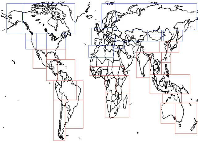
Fig. 1. Regional boxes used to build the emission maps. The boxes have been defined to distinguish areas with a fairly homogeneous

vegetation cover and fire seasonal cycle.

2 Method

The monthly emission maps have been created as follow. First, the globe is divided into boxes that contain fairly ho-mogeneous vegetation cover and fire season. The regions have been selected based upon MODIS land cover maps (http://modis-land.gsfc.nasa.gov/). In high latitude regions, the boxes follow the work of Lavou´e et al. (2000), based on state borders and dominant vegetation (blue boxes in Fig. 1). Within each box, we compute the total annual emission ac-cording to the inventories.

Similarly, we compute within each box the total number of fires detected by the ATSR instrument during the period [January 1997–May 1997] U [June 1998–December 2001]. The period from June 1997 to May 1998 was omitted since it is strongly affected by an El Ni˜no event, which resulted in very abnormal fire activity. We also removed from the datasets the ”hot-spots” occurring in the same place during several months, as those are likely to be a result of indus-trial flares. The hot-spots, likely to be agricultural or wild fires, are detected based on a simple 317 K threshold on the 3.7 µm channel on night-time observations (Arino and Melinotte, 1995). This product appears well suited for our needs as it is sensitive to fires that are small compared to the

1×1 km2pixel, and because there is no orbit drift on the plat-form, which makes possible year-to-year comparisons. On the other hand, it suffers from well-known drawbacks that are discussed in the next section. Since a cloud presence will prevent the satellite detection of an underlying fire, a cloud coverage correction was applied by weighting the number of fires by (1-C)−1where C is the monthly climatological cloud cover (New et al., 1999).

From these two datasets, we compute for each box the ra-tio between the annual emitted quantities of carbonaceous aerosols (Q) and the annual mean number of detected fires af-ter having applied the cloud cover correction (N). This Emis-sion Constant (EC) is a statistical estimate of the emitted mass per detected fire. It varies depending on the box but is assumed constant within a given box, all through the year and from one year to the next.

Using EC and the monthly hot-spot distributions at the chosen resolution, we compute an emission estimate for all months when ATSR data is available (July 1996 to January 2002 at the time of the study). In the results presented in the following, the resolution was chosen in agreement with the atmospheric model resolution (3.75×2.5 degrees in longi-tude and latilongi-tude, respectively) although the same procedure would apply to finer grids. In order to provide an emission

(4)

Fig. 2. Several proxies of biomass burning activity over Central and South America (left), Africa (center) and Australia (right). First line is

the original inventory (from Liousse et al., 1996). The two middle lines are the corrected inventories for 1998 and 2000 respectively. The bottom line is a proxy based on the estimates of burnt surfaces by GBA and GLOBSCAR (averaged value of the two is used here).

estimate for the periods when no ATSR data is available, we also computed a “climatological” monthly emission based on the mean number of fires observed during a given month for the same period that excludes El Ni˜no.

In Schultz (2002) and Duncan et al. (2003), the scaling factor is computed for each 1◦square grid box, whereas we estimate a value for each of the large regions shown in Fig. 1. In this way, the inventory emissions are redistributed over the season as in the above methods, but also within the boxes of Fig. 1. Figure 2 presents three examples of spatial redis-tribution. The first one concerns the Northern countries of South America (first row of Fig. 2). The original inventory shows a maximum of the annual estimates that extends from the Western part of Venezuela to Colombia and Ecuador. On the other hand, the ATSR-derived inventory shows for 1998 a maximum area that extends from Venezuela to Suri-name, thus largely shifted to the North-East. We also show

the ATSR corrected estimate for 2000 as a fully independent proxy of biomass burning is available for this year. The spa-tial distribution of burned surfaces (lower figure) is much closer to the ATSR corrected inventory than to the original version (top figure). This is a strong indication of the posi-tive impact of spatial redistribution. When the scaling is ap-plied on boxes that are small in comparison with typical size of biomass burning regions, as in Schultz (2002) the invento-ries are only corrected for any temporal deficiency. Duncan et al. (2003) proposed a method to account for spatial redis-tribution, which applies differently in function of the regions. For some regions the distribution of the base inventory is not modified. Other examples are shown in Fig. 2 concerning the Northern part of Africa and Australia. The three cases clearly indicate that the corrected inventory agree much better than the original with the estimates of burnt surfaces.

(5)

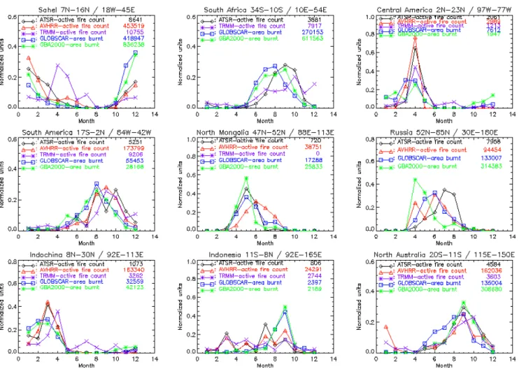
Fig. 3. Comparisons between five global fire products for nine selected regions. The number of fires for ATSR, TRMM and AVHRR and the

burnt area for GLOBSCAR and GBA2000 (in arbitrary units) are plotted as a function of time and for the year 2000. Numbers shown close to the name of the datasets correspond to the total number of occurrences (fires for ATSR, TRMM, AVHRR; burnt area for GLOBSCAR and GBA2000) detected in the year in the given region.

3 Discussion

3.1 Representativity of the night-time detection

The method provides a simple way to introduce temporal and spatial variations of biomass burning in the inventories. On the other hand, it requires unproven assumptions. A first assumption stems from the use of night observations only. As a consequence, the emission distribution is only based on fires that extend into the night. This hypothesis does not impact the mean emissions in a box as it is implicitly ac-counted for in the Emission Constant EC. On the other hand, the method will fail if the ratio between the number of day-time and night-day-time fires varies significantly, within a box, between months or between the various pixels of the emis-sion grid. To assess the representativity of the night-time fires used in this study, we have compared the global fire count products from the AVHRR (daily) (World Fire Web from the Joint Research Center of the European Commission

available at http://www.gvm.jrc.it/tem/wfw/wfw.htm), ATSR (night-time), TRMM (daily) (Giglio et al., 2003, 2000), and the GBA2000 (Gr´egoire et al., 2003) and GLOBSCAR (Si-mon et al., 2003) burnt area products. We have plotted the number of fires for ATSR, TRMM and AVHRR and the burnt area for GLOBSCAR and GBA2000 (in arbitrary units) as a function of time and for the year 2000. The comparisons are made within the large regions of Fig. 1.

Figure 3 shows the results for nine selected regions. The same plots were made for all the regions of Fig. 1. We only show a representative sample. There are two main types of proxies. ATSR, AVHRR and TRMM products are based on the detection of active fires (hot- spots). On the other hand, GLOBSCAR and GBA2000 detect the presence of burnt sur-faces. In general, there is a good agreement between the dif-ferent proxies, in particular over the major zones of biomass burning: Sahel (except TRMM), South and Central Amer-ica, Mongolia, Indochina Peninsula, and Australia (except

(6)

15 Abracos_Hill (10,75 S ; 62,35 W) 0,00 0,05 0,10 0,15 0,20 0,25 0,30 0,35 0,40 01/99 07/99 01/00 07/00 01/01 07/01 Month AOT_870

LMDZ + source LIOU AERONET LMDZ + source ATSR

Alta_Floresta (9,92 S; 56,02 W) 0 0,05 0,1 0,15 0,2 0,25 0,3 0,35 0,4 0,45 01/99 07/99 01/00 07/00 01/01 07/01 Month AOT_870

Jabiru ( 12,39 S ; 132,53 E) 0 0,05 0,1 0,15 0,2 01/00 07/00 01/01 07/01 Month AOT_870

Ilorin (8,32 N ; 4,33 E) 0 0,2 0,4 0,6 0,8 1 1,2 01/98 07/98 01/99 07/99 01/00 07/00 01/01 07/01 Month AOT_870

LMDZ+ source LIOU AERONET LMDZ + source ATSR

Mongu (15,25 S ; 23,1 0 0,05 0,1 0,15 0,2 0,25 0,3 0,35 01/97 07/97 01/98 07/98 01/99 07/99 01/00 07/00 01/01 07/01 Month AOT_870

Skukuza (24,98 S ; 31,58 E) 0,00 0,05 0,10 0,15 0,20 0,25 01/99 07/99 01/00 07/00 01/01 07/01 Month AOT_870

Figure 4. Aerosol optical thickness measured by AERONET sunphotometer (blue curve)

compared to LMDZ estimates with the new sources (red curve) and with the previous

sources (green curve).

Fig. 4. Aerosol optical thickness measured by AERONET sunphotometer (blue curve) compared to LMDZ estimates with the new sources

(red curve) and with the previous sources (green curve).

GLOBSCAR in the northern region). A few regions show significant differences between the proxies however, with the burnt area product showing an earlier season than the hot-spot based products. This feature is strongly apparent over South Africa. Note that, the optical depths – another proxy of biomass burning activity – measured by the AERONET stations Mongu (15◦S, 23◦E) and Skukuza (24◦S, 31◦E) are maximum in September and October 2000 (see Fig. 4), thus more in agreement with the hot-spot products than with the burnt area products. Indonesia is another region with strong differences between the proxies. Indeed, both burnt area product show a well-marked seasonal cycle, whereas the hot-spot products detect fire over most of the year. The three products based on the hot-spot show rather similar profiles,

with correlated month-to-month variability, so that the differ-ences cannot be attributed to the night time only detection of the ATSR.

These analyse demonstrate that in most cases, the night-time only ATSR product show a seasonal cycle that is con-sistent with the other proxies. In several cases, the burnt area products reach their maximum earlier than the fire count products. The differences between the burnt area products and those based on the hot-spots are not larger when using a night-only proxy (ATSR) than when using a night+day one (AVHRR or TRMM). This indicates that, although all prod-ucts do have uncertainties, the night time restriction does not appear to be significant.

(7)

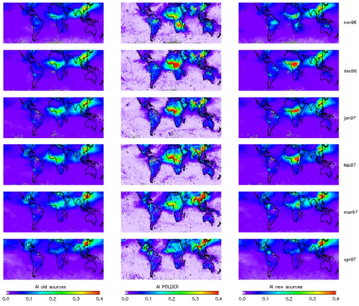
Fig. 5a. Comparisons between POLDER AI and LMDZ AI using both the original and the new sources from November 1996 to April 1997.

LMDZ AI is obtained from AOT865 assuming an Angstr¨om coefficient equal to 1.5 (Dubovik et al., 2002; Liousse et al., 1995). Note that all the monthly means are computed for the days when POLDER data are available.

3.2 Other causes of uncertainty

Cloud coverage is also a source of uncertainty as it prevents the detection of surface fires. We have attempted to correct for the cloud coverage using a monthly climatology. Nev-ertheless significant uncertainty remains as the cloud cover may differ from the climatology (in particular during spe-cific meteorological events) and also because the night-time mean cloud cover may differ from the daily climatology that we use.

Another potential problem results from the satellite cov-erage that increases with latitude (a high latitude point is sampled more frequently than a low latitude one), augment-ing the probability of fire detection. On the other hand, the boxes of Fig. 1 are small enough so that the satellite revisit

frequency does not change significantly within a box. As our method computes EC box by box, the variation of satellite coverage with the latitude is implicitly accounted for.

Moreover, the geo-location precision of the ATSR has been significantly affected during the year 2001 with a mis-registration of up to 40 km. This distance is small in com-parison with the sizes of our boxes and typical size of areas affected by biomass burning. As a consequence, misregistra-tion shall have a small impact to our results, except for areas affected by industrial flares as our detection and removal pro-cedure is based on a persistent signal within a 3 km radius.

Finally, these maps have been made assuming that in each box, the emission efficiency of fires for BC or OC has no seasonal or interannual variation (EC is constant). This is

(8)

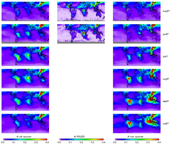
Fig. 5b. Comparisons between POLDER AI and LMDZ AI using both the original and the new sources from May 1997 to October 1997.

LMDZ AI is obtained from AOT865 assuming an Angstr¨om coefficient equal to 1.5 (Dubovik et al., 2002; Liousse et al., 1995). Note that all the monthly means are computed for the days when POLDER data are available.

a rather strong assumption as, for a given vegetation type, the emitted quantities depend on several parameters such as ground humidity, vegetation state or burns history, that vary with the season.

4 Results and validation

Both original and satellite-corrected emission maps have been used as input of the Laboratoire de M´et´eorologie Dy-namique (LMD) General Circulation Model, LMDz, coupled with INCA (Interaction with Chemistry and Aerosols) which is an emission/chemistry model (http://www.ipsl.jussieu.fr/

∼_{dhaer/inca/). We use the model with a resolution of 96×72}

(3.75×2.5 degrees in longitude and latitude) and 19 hybrid vertical levels. Only carbonaceous aerosols were analyzed

in this study. The model can include its own dynamics, al-though we nudged here the meteorological fields from the 6-hourly ECMWF reanalysis. It generates fields of aerosol load [g.m−2] that are converted into optical thicknesses at 865 nm using constant factors (3.5 m2.g−1for OC and 4.5 m2.g−1for BC, (Dubovik et al., 2002; Liousse et al., 1995, 1996) based on typical size distributions of biomass burning aerosols.

4.1 Seasonal cycle

Ground-based measurements from AERONET (Holben et al., 1998) stations in South America, Africa and Australia are used to validate our simulations. Chin et al. (2002) evaluates the simulations of the GOCART aerosol transport model, using biomass burning emissions from Duncan et al. (2003),

(9)

for the different aerosol components through a comparison to AERONET data. More than 20 AERONET sites are used for the comparison, although only five of them are significantly affected by biomass burning emissions. Here, we show sev-eral seasonal cycles whereas Chin et al. (2002) only analyze a mean cycle. These year-to-year comparisons are essential as there is significant interannual variability, which results both from the emissions and the meteorology. Comparisons are also made with satellite observations from the POLDER (POLarization and Directionality of the Earth Reflectances, Deschamps et al., 1994) spaceborne instrument, which is well suited to study aerosols and in particular biomass burn-ing aerosols. The Aerosol Index (AI) from POLDER (Deuz´e et al., 2001), available both over land and ocean, is an indi-cator of submicronic aerosol load only, thus mainly sulfate, BC and OC. The analysis of POLDER retrievals (Tanr´e et al., 2001) provides a rough identification of the aerosol origin.

Figure 4 shows the mean AERONET Aerosol Optical Thickness at 870 nm (AOT870) (in blue), the simulation re-sults using the new sources (red) and those using the previous sources from Liousse et al. (1996) (in green) at six differ-ent AERONET sites. Two type of information are shown in Fig. 4. First, the information on the phase of the burning season. The improvements to the seasonal cycle are given by the phasing of the simulated curves (red and green) with the observation curve (blue). The other information concerns the aerosol load, which is directly linked to the amplitude of the curves. The method presented here only impacts the spa-tial and temporal distribution of fires but not the mean emit-ted quantities as we assume the total annual estimates of the original inventory to be correct averaged estimates.

In a first step, we discuss the results over South America, where Alta Floresta (9◦_{S, 56}◦_{W) and Abracos Hill (10}◦_S,

62◦W) are selected because long-time series of data are available. AERONET data show the impact of the biomass burning activity from August to November with a maximum value generally in September during three consecutive years from 1999 to 2001. The correction of the emission inven-tories using the satellite data shift the period with a large aerosol load by typically two months. Although there are some disagreement in terms of optical thickness between the simulations and the sunphotometer measurements, in partic-ular during the later part of the burning season, the cycle is clearly improved. The observed aerosol load cycle for the year 2000 is clearly different than for the other years. It is not reproduced by the simulation. On the other hand, none of the biomass burning proxies (see Fig. 3) shows a significant burning activity during the later part of the year, while a large aerosol load is observed. Therefore, none method based on these satellite products would reproduce this specific event.

Over Australia, Jabiru (12◦S, 132◦E) is the only site in the North with sufficient amount of data. Although the seasonal cycle is not complete, the maximum aerosol load appears to be in September and October. In addition, the compar-isons of the diverse global fire products (see Fig. 3) show that

the burning season starts in May/June and ends in November with the maximum of detected fire from August to October. Note that only GLOBSCAR show relatively large amount of fire earlier (in June and July) in disagreement with GBA2000 and all fire count products. Hence, methods based on the other fire products (except GLOBSCAR) would have repro-duced a similar seasonal cycle. The corrected emission maps lead to a better agreement of the seasonal cycle with the different biomass burning proxies over North Australia al-though the magnitude of the optical depth is somewhat too small.

Over the African continent there are two main areas of biomass burning. One extends along 10◦of latitude with the main activity between November and February. The other large burning area of Africa extends over the southern sub-tropics, with an activity that starts in June in the western part of the area, moves to the East and Madagascar, and ends in November. Figure 4 shows the comparison results over Ilorin (8◦N, 4◦E), Mongu (15◦S, 23◦E) and Skukuza (24◦S, 31◦E) sites, which were chosen for their extended time series. These comparisons indicate that the original emission maps show a satisfactory seasonal cycle that is not improved nor degraded using the information from the ATSR. On the other hand, the modeled optical thicknesses are much smaller than the observations, which can be a result of an underestimate of the emission fluxes, although the fac-tor used to convert masses to optical thicknesses can also be blamed. Chin et al. (2002) show that Ilorin is also influenced by dust aerosols, which are not included in the simulations.

In order to have a global view of the representation of carbonaceous aerosols in the model, we show on Figs. 5a and b a comparison between POLDER AI (a good index for carbonaceous and sulfate aerosols) and LMDZ AI. The sim-ulation overlaps the period of the POLDER data, i.e. from November 1996 to October 1997. For consistency with the satellite measurements, the model simulates the source and cycle of carbonaceous and sulfate (Boucher et al., 2002) aerosols. The global picture confirms several findings of the AERONET comparisons. Figure 5a shows that both invento-ries depict correctly the phase of the aerosol load seasonal cy-cle in Western Africa, although the maximum of the aerosol index is shifted to the East in February in the simulation (new sources). In South Africa, the model seems to under predict the aerosol index in June (Fig. 5b). The satellite data confirm that there is no significant aerosol load over South America from May to June (see middle panel on Fig. 5b). The model predictions using the ATSR-derived inventory are in agree-ment with observations, contrary to what the model predicts with the original sources in May and June. The use of infor-mation from ATSR fires brings about an even larger change in the phasing of biomass burning over North Australia. The original sources yield a significant aerosol load from May to September, when the corrected sources indicate that the fire activity starts in September.

(10)

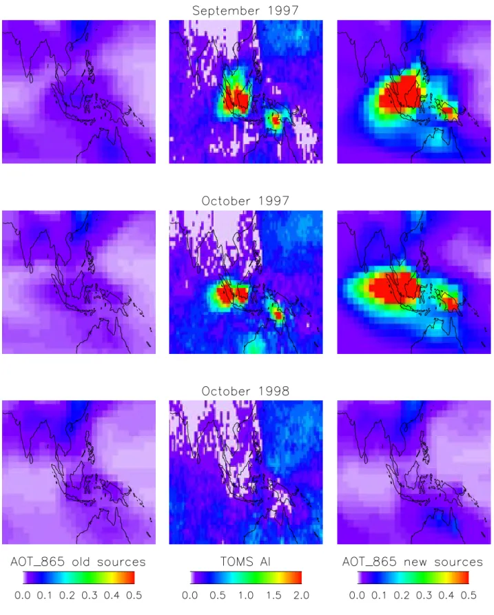
18 Figure 6. Comparison of the aerosol index from the Earth-Probe TOMS (middle panels) with

simulated aerosol optical depths at 865 nm simulated with Liousse et al. (1996) inventory

(left panels) and newly derived sources from ATSR fire counts (right panels). Color scales

were chosen from 0 to 2 for TOMS AI and from 0 to 0.5 for LMDZ AOT in order to be

consistent with the assumed value of 5 for the slope of the fit between the TOMS AI and the

AOT at 865 nm based upon the Chiapello et al. (2000) study.

Fig. 6. Comparison of the aerosol index from the Earth-Probe TOMS (middle panels) with simulated aerosol optical depths at 865 nm

simulated with Liousse et al. (1996) inventory (left panels) and newly derived sources from ATSR fire counts (right panels). Color scales were chosen from 0 to 2 for TOMS AI and from 0 to 0.5 for LMDZ AOT in order to be consistent with the assumed value of 5 for the slope of the fit between the TOMS AI and the AOT at 865 nm based upon the Chiapello et al. (2000) study.

(11)

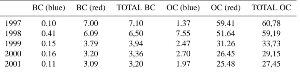
Table 1. Quantities of carbonaceous aerosols emitted by biomass burning (including savanna, forest and agricultural fires) in the

ATSR-derived inventory. BC emissions are in Tg of Carbon (TgC) per year and OC emissions are in Tg of mass (Tg) per year. BC and OC (blue) correspond to the emissions of the blue boxes of Fig. 1 (boreal latitudes) and BC and OC (red) to the emissions of the red boxes

BC (blue) BC (red) TOTAL BC OC (blue) OC (red) TOTAL OC

1997 0.10 7.00 7,10 1.37 59.41 60,78 1998 0.41 6.09 6,50 7.55 51.64 59,19 1999 0.15 3.79 3,94 2.47 31.26 33,73 2000 0.16 3.20 3,36 2.70 26.45 29,15 2001 0.11 3.09 3,20 1.97 25.48 27,45 4.2 Interannual variability

Table 1 summarizes the emitted quantities of carbonaceous aerosols in the new ATSR-derived inventory for each year of ATSR observations. We have assumed that the total an-nual estimates of the original inventories (Liousse et al., 1996 and Lavou´e et al., 2000) – as climatological averaged values – are correct. In the original Liousse et al. (1996) inven-tory, emissions represent 35.2 Tg of OC and 4.63 Tg of BC (including savanna, tropical forests and agricultural fires; ex-cluding domestic fuels). Year 1999 compares well with these estimates whereas years 1997 and 1998 are a factor 1.5–1.7 larger than the averaged values. This increase in the emis-sions is mostly due to the Indonesian fires event of Septem-ber/October 1997. On the other hand, emissions of 2000 and 2001 are smaller (factor of 0.65 to 0.75) than those of the climatological year.

In order to show that the proposed method accounts for large interannual variations, we now focus on the partic-ular event of Indonesian fires that took place in Septem-ber/October 1997 (Nakajima et al., 1999), thought to be a consequence of 1997/1998 El Ni˜no. This phenomenon was well captured by the Earth-Probe TOMS (Herman et al., 1997). Figure 6 shows a comparison between TOMS AI and LMDZ AOT865 based upon the Liousse et al. (1996) inventory and upon the ATSR-derived inventory. Note that although an exact quantitative comparison is difficult, the emissions from these fires are reproduced qualitatively through the use of ATSR fire counts. TOMS measurements indicate a large aerosol load over Indonesia in September and October 1997. The consequence of the abnormal fire activity is not depicted with the original inventory, as one would expect for a climatological source. By contrast, the use of ATSR-based emission maps leads to an aerosol in-dex significantly larger than for other years (i.e. October 1998 in Fig. 6). We note also that the spatial distribution of the aerosol loads compares well with the TOMS obser-vations. In addition, Nakajima et al. (1999) have estimated from the AVHRR data that the region of optical thickness at 500 nm larger than 0.5 reaches the Indian and Australian coasts and covers an area such as 2000×5000 km2. Such high optical depths have been observed from September to November 1997. Hence, the spatial distribution of the fire

event reproduced by the simulation seems correct although the optical depths appear overestimated. This comes from an overestimation of the emissions due to a high EC computed for the Indonesian region. A possible explanation is that too low fires are detected during “normal years”, which might be due to high cloud cover (65% to 85%) over Indonesia.

5 Conclusions

The method described in this paper provides a simple way to introduce biomass burning seasonal cycles into already ex-isting inventories and to take into account interannual varia-tions. The comparison of the aerosol transport simulations to in-situ and satellite measurements clearly shows an improve-ment when using the fire count information. In particular, the aerosol load seasonal cycle over South America and Aus-tralia, which are not well represented in the original invento-ries, are now better depicted. The comparison with POLDER products provides a global and qualitative validation of the seasonal cycle of biomass burning aerosol. Due to the rather short observing period of POLDER-1, the analysis of the sea-sonal cycle is incomplete, and we are expecting additional information from the recently launched POLDER-2 instru-ment onboard ADEOS-II. The comparison of the model sim-ulations with AERONET data allows more quantitative com-parison over specific sites. These comcom-parisons confirm the improvement when using the fire count data to constrain the seasonal cycle and the inter-annual events, although signifi-cant discrepancies were found in the amplitude of the aerosol load in particular toward the end of the biomass burning sea-son.

The present study focuses on the use of ATSR data because a five years period was available at the time of our analysis. A comparison of this biomass burning proxy to others, limited to the year 2000, indicate a general good agreement. The derivation of aerosol emission from burnt surfaces requires less assumption than from hot-spot counts. Global invento-ries of aerosol emission from such datasets as GLOBSCAR (Hoelzemann et al., 2003) will be of particular interest when multi-year estimates become available.

(12)

Acknowledgements. The emission factors are based on the ATSR

World Fire Atlas managed by the European Space Agency (ESA). We thank Cathy Liousse for providing the OC and BC emission inventories. We thank the principal investigators Brent Holben, Paulo Artaxo, Ross Mitchell and Rachel Pinker and the AERONET program team for providing the ground-based aerosol data used in this work. The satellite data come from the POLDER instrument developed by the Centre National d’Etudes Spatiales onboard the ADEOS platform developed by NASDA.

References

Arino, O. and Melinotte, J. M.: Fire index atlas, Earth observation quaterly, 50, 1995.

Boucher, O., Pham, M., and Venkataraman, C.: Simulation of the atmospheric sulfur cycle in the Laboratoire de M´et´eorologie Dy-namique General Circulation Model. Model description, model evaluation, and global and European budgets, Note scientifique de l’IPSL, 23, 2002 (available at http://www.ipsl.jussieu.fr/poles/ Modelisation/NotesSciences.htm).

Br´eon, F.-M., Tanr´e, D., and Generoso, S.: Aerosol effect on cloud droplet size monitored from satellite, Science, 295, 834–838, 2002.

Charlson, R. J., Schwartz, S. E., Hales, J. M., Cess, R. D., Coakley, J. A. J., Hansen, J. E., and Hofmann, D. J.: Climate forcing by anthropogenic aerosols, Science, 255, 423–430, 1992.

Chiapello, I., Goloub, P., Tanr´e, D., Marchand, A., Herman, J., and Torres, O.: Aerosol detection by TOMS and POLDER over oceanic regions, Journal of Geophysical Research – Atmo-spheres, 105, 7133–7142, 2000.

Chin, M., Ginoux, P., Kinne, S., Torres, O., Holben, B. N., Dun-can, B. N., and Martin, R. V., Logan, J. A., Higurashi, A., and Nakajima, T.: Tropospheric aerosols optical thickness from the GOCART model and comparisons with satellite and sun pho-tometer measurements, Journal of the Atmospheric Sciences, 59, 461–483, 2002.

Cooke, W. F., Koffi, B., and Gr´egoire, J.-M.: Seasonality of vegeta-tion fires in Africa from remote sensing data and applicavegeta-tion to a global chemistry model, Journal of Geophysical Research, 101, 21 051–21 065, 1996.

Deschamps, P.-Y., Br´eon, F.-M., Leroy, M., Podaire, A., Bricaud, A., Buriez, J.-C., and S`eze, G.: The POLDER mission: instru-ment characteristics and scientific objectives, IEEE Transactions on geoscience and remote sensing, 32, 598–615, 1994.

Deuzé, J. L., Bréon, F.-M., Devaux, C., Goloub, P., Herman, M., Lafrance, B., Maignan, F., Marchand, A., Nadal, F., Perry, G., and Tanré, D.: Remote sensing of aerosols over land surfaces from POLDER-ADEOS-1 polarized measurements, Journal of Geophysical Research, 106, 4913–4926, 2001.

Dubovik, O., Holben, B., Eck, T. F., Smirnov, A., Kaufman, Y. J., King, M. D., Tanr´e, D., and Slutsker, I.: Variability of ab-sorption and optical properties of key aerosol types observed in worldwide locations, Journal of the Atmospheric Sciences, 59, 590–608, 2002.

Duncan, B. N., Randall, V. M., Staudt, A. C., Yevich, R., and logan, J. A.: Interannual and seasonal variability of biomass burning emissions constrained by satellite observations, Journal of Geo-physical Research, 108, 4040, doi:10.129/2002JD002378, 2003.

Giglio, L., Kendall, J. D., and Mack, R.: A multi-year active fire data set for the tropics derived from the TRMM VIRS, Interna-tional Journal of Remote Sensing, in press, 2003.

Giglio, L., Kendall, J. D., and Tucker, C. J.: Remote sensing of fires with the TRMM VIRS, International Journal of Remote Sensing, 21, 203–207, 2000.

Gr´egoire, J.-M., Tansey, K., and Silva, J. M. N.: The GBA2000 initiative: Developing a global burned area database from SPOT-VEGETATION imagery, International Journal of Remote Sens-ing, 24, 1369–1376, 2003.

Haywood, J. and Boucher, O.: Estimates of the direct and indirect radiative forcing due to tropospheric aerosols: a review, Reviews of Geophysics, 38, 513–543, 2000.

Herman, J. R., Bhartia, P. K., Torres, O., Hsu, C., Seftor, C., and Celarier, E.: Global distribution of UV-absorbing aerosols from Nimbus 7/TOMS data, Journal of Geophysical Research, 102, 16 911–16 922, 1997.

Hoelzemann, J. J., Brasseur, G. P., Granier, C., Schultz, M. G. and Simon, M.: The Global Wildfire Emission Model GWEM: a new approach with global area burnt data, Journal of Geophysical Re-search, submitted, 2003.

Holben, B. N., Eck, T. F., Slutsker, I., Tanr´e, D., Buis, J. P., Set-zer, A., Vermote, E., Reagan, J. A., Kaufman, Y. J., Nakajima, T., Lavenu, F., Jankowiak, I., and Smirnov, A.: AERONET – A federated intrument network and data archive for aerosol charac-terization, Remote Sensing of Environment, 66, 1–16, 1998. IPCC, Climate change 2001: The scientific basis, contribution of

working group I to the third assessment. Report of the Intergov-ernmental Panel on Climate Change, Cambridge university press, New York, USA, 881 pp. 2001.

Lavou´e, D., Liousse, C., Cachier, H., Stocks, B. J., and Goldammer, J. G.: Modeling of carbonaceous particles emitted by boreal and temperate wildfires at northern latitudes, Journal of Geophysical Research, 105, 26 871–26 890, 2000.

L´eon, J.-F., Chazette, P., Pelon, J., Dulac, F., and Randriamiarisoa, H.: Aerosol direct radiative impact over the INDOEX area based on passive and active remote sensing, Journal of Geophysical Re-search, 107, 10129, doi:10.1029/2000JD000116, 2002. Liousse, C., Devaux, C., Dulac, F., and Cachier, H.: Aging of

sa-vanna biomass burning aerosols: consequences on their optical properties, Journal of Atmospheric Chemistry, 22, 1–17, 1995. Liousse, C., Penner, J. E., Chuang, C., Walton, J. J., Eddleman,

H., and Cachier, H.: A global three-dimensional model study of carbonaceous aerosols, Journal of Geophysical Research, 101, 19 411–19 432, 1996.

Nakajima, T., Higurashi, A., Takeuchi, N., and Herman, J. R.: Satel-lite and ground-based study of optical properties of 1997 Indone-sian forest fire aerosols, Geophysical Research Letters, 26, 2421– 2424, 1999.

New, M., Hulme, M., and Jones, P.: Representing twentieth-century space-time climate variability. Part I: Development of a 1961– 90 mean monthly terrestrial climatology, Journal of Climate, 12, 829–856, 1999.

Schultz, M. G.: On the use of ATSR fire count data to estimate the seasonal and interannual variability of vegetation fire emissions, Atmospheric Chemistry and Physics, 2, 387–395, 2002. Simon, M., Plummer, S., Fierens, F., Hoelzemann, J. J., and Arino,

O.: Burnt area detection at global scale using ATSR-2: the GLOBSCAR products and their qualification, Journal of

(13)

physical Research, submitted, 2003.

Tanré, D., Bréon, F.-M., Deuzé, J. L., Herman, M., Goloub, P., Nadal, F., and Marchand, A.: Global observation of anthro-pogenic aerosols from satellite, Geophysical Research Letters, 28, 4555–4558, 2001.

Twomey, S.: The influence of pollution on the shortwave albedo of clouds, Journal of the Atmospheric Sciences, 34, 1149, 1977.