HAL Id: halshs-01998001
https://halshs.archives-ouvertes.fr/halshs-01998001
Preprint submitted on 29 Jan 2019
HAL is a multi-disciplinary open access
archive for the deposit and dissemination of sci-entific research documents, whether they are pub-lished or not. The documents may come from teaching and research institutions in France or abroad, or from public or private research centers.
L’archive ouverte pluridisciplinaire HAL, est destinée au dépôt et à la diffusion de documents scientifiques de niveau recherche, publiés ou non, émanant des établissements d’enseignement et de recherche français ou étrangers, des laboratoires publics ou privés.
Eliciting Choice Correspondences A General Method
and an Experimental Implementation
Elias Bouacida
To cite this version:
Elias Bouacida. Eliciting Choice Correspondences A General Method and an Experimental Imple-mentation. 2019. �halshs-01998001�
WORKING PAPER N° 2019 – 09
Eliciting Choice Correspondences
A General Method and an Experimental Implementation
Elias Bouacida
JEL Codes: C91, D01, D60
Keywords : choice correspondences, revealed preferences, welfare,
indifference, WARP, justnoticeable preferences, aggregation of preferences
P
ARIS-
JOURDANS
CIENCESE
CONOMIQUES48, BD JOURDAN – E.N.S. – 75014 PARIS
TÉL. : 33(0) 1 80 52 16 00= www.pse.ens.fr
CENTRE NATIONAL DE LA RECHERCHE SCIENTIFIQUE – ECOLE DES HAUTES ETUDES EN SCIENCES SOCIALES ÉCOLE DES PONTS PARISTECH – ECOLE NORMALE SUPÉRIEURE
Eliciting Choice Correspondences
A General Method and an Experimental Implementation
Elias Bouacida
∗November, 2018
Abstract
I introduce a general method for identifying choice correspondences experimentally, i.e., the
sets of best alternatives of decision makers in each choice sets. Most of the revealed preference
literature assumes that decision makers can choose sets. In contrast, most experiments force the choice of a single alternative in each choice set. In this paper, I allow decision makers to choose several alternatives, provide a small incentive for each alternative chosen, and then randomly select one for payment. I derive the conditions under which the method at least partially identifies the choice correspondence, by obtaining supersets and subsets for each choice set. I illustrate the method with an experiment, in which subjects chose between four paid tasks. I can retrieve the full choice correspondence for 26% of subjects and bind it for another 46%. Subjects chose sets of size 2 or larger 60% of the time, whereas only 3% of them always chose singletons. I then show that 46% of all observed choices can be rationalized by complete, reflexive and transitive preferences in my experiment, i.e., satisfy the Weak Axiom of Revealed Preferences – WARP hereafter. Weakening the classical model, incomplete preferences or just-noticeable difference preferences do not rationalize more choice correspondences. Going beyond WARP, however, I show that complete, reflexive and transitive preferences with menu-dependent choices rationalize 93% of observed choices. Having elicited choice correspondences allows me to conclude that indifference is widespread in the experiment. These results pave the way for exploring various behavioral models with a unified method.
JEL Codes: C91, D01, D60
keywords: choice correspondences, revealed preferences, welfare, indifference, WARP, just-noticeable preferences, aggregation of preferences.
∗Paris School of Economics, University Paris 1 Panthéon Sorbonne. [email protected] I am grateful to Jean-Marc Tallon, Daniel Martin and Stéphane Zuber for their invaluable advice and guidance. I want to thank Maxim Frolov for his help during the experiment. I am also grateful to all the people I have interacted with during the course of my Ph.D., among them Eric Danan, Peter Klibanoff, Marco Mariotti, Pietro Ortoleva, Nicolas Jacquemet, Béatrice Boulu-Reshef, Daniele Caliari, Philippe Colo, Quentin Couanau, Guillaume Pommey, Julien Combe, Shaden Shebayek, Rémi Yin, Justine Jouxtel, and Antoine Hémon. I want to thank seminar participants of the Roy seminar, TOM seminar, and Workgroup on experiments at Paris School of Economics. I would also like to thank seminar participants at Paris Nanterre University as well as conference participants and discussants at AFSE 2018, BRIC 2018, ASFEE 2018, Queen Mary University Ph.D. Workshop, FUR 2018, SARP 2018, ESA 2018 and Econometric Society European Meeting 2018. I acknowledge the support of ANR projects CHOp (ANR-17-CE26-0003) and DynaMITE (ANR-13-BSH1-0010) and Labex OSE (10-LABX-0093). All errors are mine.
Introduction
In a seminal paper, Samuelson (1938) introduced the revealed preferences method. He linked preferences and choices by positing that chosen alternatives are better than unchosen ones, thus revealing the preference of the decision maker. In experiments, and in most real-life settings, choices are elicited using a choice function: the decision maker chooses one alternative from the choice set, i.e., the set of available alternatives. In principle, however, choices are commonly modeled with a choice correspondence: the decision maker chooses a non-empty set from the choice set.1
Arrow (1959) gave the condition under which a choice correspondence, or a choice function, can be rationalized by a reflexive, complete, and transitive preference, i.e., a classical preference, the Weak Axiom of Revealed Preferences – WARP hereafter. Roughly, WARP states that if an alternative x is revealed better – i.e., preferred – to another alternative y, it cannot be the case that from another choice, y is revealed preferred to x.
In this paper, I introduce pay-for-certainty, a direct method for identifying choice correspondences. I allow decision makers to choose several alternatives, provide a small incentive for each alternative chosen, and then randomly select one for payment. Previous methodologies used a proxy to do so, preference for flexibility in Danan and Ziegelmeyer (2006) and Costa-Gomes et al. (2016), repeated choices in Agranov and Ortoleva (2017), or delegation to a random device in Qiu and Ong (2017), Sautua (2017), and Cettolin (2016). These methodologies might fail to identify indifference between two alternatives precisely.
Identifying a choice correspondence for each decision maker allows me to explore new questions. First, classical preferences often fail in practice to rationalize observed behavior. It is natural to look for which assumption might explain its failure. I study relaxations of completeness, transitivity of the indifference and menu-independence, using testable conditions on choice correspondences provided by Eliaz and Ok (2006) and Aleskerov, Bouyssou, and Monjardet (2007). Second, having identified choice correspondences, I can study indifference directly and assess how widespread it is. Third, with choice functions, decision makers have at most one maximal alternatives, whereas with choice correspondences, they might have more than one. The more extensive set of Pareto-superior alternatives opens up more room for agreement in collective decision making. Agreement between decision makers should be more accessible, as each has potentially several Pareto-superior alternatives.
Choice correspondences cannot be obtained directly. A direct method would allow decision makers to choose several alternatives and then randomly select one for payment. This method might not identify their choice correspondence in the presence of indifference or incompleteness, as a simple example illustrates. Julia is a decision maker who likes equally coffee and tea. According to 1One real-life example of the choice of a non-empty set from the choice set is approval voting. Decision makers can vote for all the candidate they deem acceptable.
this simple identification method, she can choose {coffee}, {tea} or {coffee, tea} in the choice set {coffee, tea}. Each chosen set has the same payoff for her. This creates a uniqueness problem. This procedure does not guarantee that the decision maker chooses all maximal – i.e., Pareto-superior – alternatives. On the other hand, revealed preference models (see, for instance, Sen (1971), Nehring (1997)) assume that the chosen set is the set of maximal alternatives.
Pay-for-certainty solves the uniqueness problem by incentivizing decision makers to choose all maxi-mal alternatives. For each alternative chosen, the decision maker earns an additional payment ε > 0. In the previous example, Julia is better off by choosing {coffee, tea} and getting coffee or tea and 2ε in additional payment rather than choosing and getting {coffee} or {tea} and ε. The full char-acterization of pay-for-certainty is thus:
In each set of alternatives, the decision maker chooses all the alternatives she wishes. She earns an additional payment of $ε by chosen alternatives. The alternative she gets is selected from her chosen alternatives using, for instance, a uniform random draw.
The additional payment of pay-for-certainty implies forgone gains when the chosen set is not the whole set. Choosing only one alternative earns ε, whereas choosing two earns 2ε, and so on. I show that under mild monotonicity conditions, the decision maker chooses all maximal alternatives. A possible downside is that some chosen alternatives might not be maximal if ε is large and the differences among the (direct) payoffs of some alternatives are within ε of each other. The method shares many features with the experiment of Costa-Gomes et al. (2016), but there are some key differences. First, choosing several alternatives implies a gain, not a loss. Second, the gain here will be much lower in magnitude, theoretically eliciting more indifference relations. Last, the dominant strategy of a decision maker who is indifferent between different alternatives is to choose all of them. Under the assumptions of transitive strict preferences, monotonicity for the gains, and constrained maximization of the additional payment, pay-for-certainty (partially) identifies the choice corre-spondence. Importantly, I do not assume completeness of the preference nor transitivity of the in-difference relation. Constrained maximization is not directly testable. Instead, I provide a testable implication of all the assumptions I make: increasing chosen set. Increasing chosen set captures the intuitive idea that, for a given choice set, the larger the additional payment is, the larger the chosen set should be. Hence, for a given choice set, the chosen set with pay-for-certainty with no additional payment is a subset of the set of maximal alternatives, while it is a superset of the set of maxi-mal alternatives when the additional payment is positive. When increasing chosen set is verified, I partially identify the choice correspondence of the decision maker. I precisely identify maximal alternatives in a given set when the two are equal. I fully identify the choice correspondence of a decision maker when for all choice sets, I precisely identify all maximal alternatives. I will call the choice correspondence of the decision maker the fully identified ones, otherwise mentioning that the identification was only partial.
I have carried out an experiment to illustrate pay-for-certainty in the laboratory. The 223 subjects of the experiment chose between four tasks they had to perform at the end of the session. They were rewarded depending on their performance in the tasks. Subjects chose in all of the 11 possible subsets of tasks in order to fully identify their choice correspondence. Subjects chose three times in the same sets to test the two identification assumptions: twice with different strictly positive additional payments and once with no additional payment. The computer selected one of the 33 choices randomly for the payment and drew the task they performed from the chosen set randomly. I also ran an experiment with the same tasks but forcing the choice of singletons, which amounts to identifying a choice function. Finally, I varied the information provided about the tasks to study the influence of the quality and quantity of information on the choices.
In the experiment, subjects did not choose singletons when not constrained to do so. 60% of all choices were not singletons, and only 3% of subjects always chose singletons. Importantly, even without incentive to choose multiple alternatives, in the 0-correspondence case, the choice of non-singletons does not disappear. It also remained when the information provided was quite complete. Overall, I identify the choice correspondence of 26% of subjects and at least partially identify it for 72% of subjects.
Descriptively, reflexive, transitive and complete preferences together often fail to explain observed choices. Normatively, the appeal of some assumptions is also dubious. Aumann (1962) and Bewley (2002) have criticized complete preferences. Similarly, Armstrong (1939) and Luce (1956) criticized transitive indifference and introduced just-noticeable difference modeling in response. Sen (1997) was critical of menu-independent (i.e., set-independent) maximization. In the last decade, the theoretical literature on incomplete preferences blossomed, following Ok (2002) and Bewley (2002), but few empirical studies have been conducted.2 Similarly, just-noticeable difference and
menu-dependent model have seldom been explored.3 Identifying the choice correspondence of a decision
maker allows me to explore these assumptions.
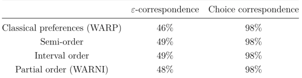
First, classical preferences rationalize 98% of (fully identified) choice correspondences, leaving al-most no room for alternative modeling of preferences. It represents only 26% of the subjects of my experiment, however. For the remaining ones, I will explore the alternative models on their choices with additional payments, which I will call hereafter the ε-correspondence. Only 46% of the ε-correspondences satisfy WARP. I use choice correspondences to study incomplete preferences directly, using the Weak Axiom of Revealed Non-Inferiority – WARNI hereafter. It is equivalent to rationalizability by a reflexive and transitive preference, a corollary to Eliaz and Ok (2006)’s 2To the best of my knowledge, five experiments are looking at incomplete preferences (Danan and Ziegelmeyer (2006), Cettolin (2016), Costa-Gomes et al. (2016), Qiu and Ong (2017), Sautua (2017)). Only one of them, by Costa-Gomes et al. (2016), looked at alternatives in the certain domain.
3Models of status-quo bias, attraction and decoy effects, and so on, are menu-dependent models of choice, but they always assume the impact of the menu-effect. Here I am thinking of the effect of the menu per se, not assuming the mechanism behind the effect of the menu.
Theorem 2. Incomplete preferences rationalize 49% of ε-correspondences. Second, I study just-noticeable difference models, formalized by Luce (1956) and Fishburn (1970) among others. The “coffee and sugar” example4 captures the intuition behind just-noticeable difference models. The
difference between the two alternatives might be imperceptible, but the addition of imperceptible differences might be perceptible. I use Aleskerov, Bouyssou, and Monjardet (2007) testable impli-cations of just-noticeable difference. In my experiment, just-noticeable difference and incomplete preferences rationalize the same choice correspondences and ε-correspondences. Both rationalize only marginally more than classical preferences. This result is close to the proportion obtained by Costa-Gomes et al. (2016), in the context of sure outcomes, but in contrast with the rest of the literature (Danan and Ziegelmeyer (2006), Cettolin (2016), Sautua (2017) and Qiu and Ong (2017)) which use risky or ambiguous lotteries to study incomplete preferences.
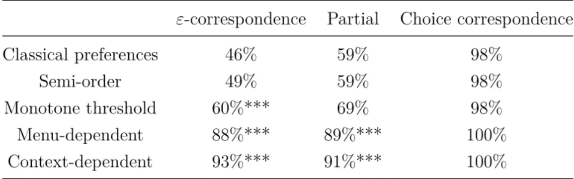
Finally, I relax menu-independence. I study the models of Frick (2016) and Aleskerov, Bouyssou, and Monjardet (2007). They are variations on just-noticeable difference models, but now the threshold to be noticed might depend on the menu and the alternatives considered. The easiest one to satisfy, the context-dependent model of Aleskerov, Bouyssou, and Monjardet (2007), rationalizes up to 93% of ε-correspondences, while not being a void requirement on choice correspondences.5
It reveals reflexive, complete and transitive preferences. In this model, however, decision makers might sometimes choose sub-optimal alternatives.
Identifying the choice correspondence also allows me to study indifference. It matters as a decision maker might violate WARP with choice functions if she has classical preferences with indifference. The following example illustrates why.
Example: Singleton choice Julia is indifferent between three hot drinks, coffee, tea, and hot chocolate, and she randomizes when she is indifferent and forced to choose one alternative. I identify her choice function, by forcing her to choose singletons. Her observed choices are: c({coffee, tea, hot chocolate}) = {tea}, c({coffee, tea}) = {coffee}, c({coffee, hot chocolate}) = {hot chocolate}, and c({tea, hot chocolate}) = {tea}. This choice pattern does not sat-isfy WARP, and the revealed preferences of Julia are coffee∼tea, tea∼hot chocolate, and coffee≻hot chocolate.6 Singleton choices do not reveal Julia’s preferences, and I deem her
“irrational” because I have forced her to choose singletons.
Forcing decision makers to choose one alternative can generate this kind of error. Danan (2008) explains under which conditions on the behavior of the decision maker a choice function successfully 4Luce (1956): “Find a subject who prefers a cup of coffee with one cube of sugar to one with five cubes (this should not be difficult). Now prepare 401 cups of coffee with(1 + 100i )x grams of sugar, i = 0, 1, . . . , 400, where x is the weight of one cube of sugar. It is evident that he will be indifferent between cup i and cup i + 1, for any i, but he is not indifferent between i = 0 and i = 400.”
5See AppendixC.3.1for a study of the explanatory power of the different models on choice correspondences. 6There are different possibilities to assess revealed preferences, as shown in Sen (1971). I use Arrow (1959)’s definition of revealed preferences.
assesses her rationality.
Experimentally, the restriction of choice to singletons is not what explains violations of WARP, as 46% of correspondences and 57% of all singleton choices satisfy WARP. Choices with ε-correspondences are more difficult than with singletons, which probably explained the insignifi-cant decrease in the satisfaction of WARP.7 On the other hand, the restriction to singleton choice
significantly changes the revealed preferences. On average, for ε-correspondences and choice corre-spondences that satisfy WARP, 50% of comparisons between alternatives are indifference relations. If I use preferences obtained with the context-dependent model of Aleskerov, Bouyssou, and Mon-jardet (2007), when it rationalizes ε-correspondences, 36% of comparisons are indifference relations. Indifference relations have a significant share of revealed preference relations. It is likely to imply that the number of Pareto-superior alternatives for each decision maker is more substantial than usually assumed, which is relevant for individual welfare analysis.
This identification of indifference has positive consequences for collective welfare analysis as well. By allowing subjects to have more than one maximal alternatives, choice correspondences facilitate the agreement among decision makers compared to choice functions. 73% of choice correspondence who satisfy WARP agree that the addition task and the spellcheck task are the best alternatives. This proportion is much higher than when I identify choice functions which satisfy WARP. In that case, the most preferred agreed upon task is the copy task, and 31% of subjects prefer it. These results show that in practice, an agreement between decision makers is more accessible with choice correspondences. It is a result in the spirit of the one proved by Danan, Gajdos, and Tallon (2013) for incomplete preferences.
The paper is structured as follows. Section1characterizes the domain of application of the pay-for-certainty method, as well as testable consequences of the assumptions I make. Section 2 describes the experiment. Section3studies the identification of choice correspondences in practice. Section4 studies classical preferences and then alternative rationalization of choice correspondences. Section 5 explores the prevalence of indifference. Section 6 explores the aggregation of preferences and choices with choice correspondences. Section 7 concludes.
1
Method
In this section, I describe the pay-for-certainty method and lay down the conditions under which it allows me to identify the choice correspondence of a decision maker.
7If we compare all possible choice correspondences and all possible choices functions and pick one at random in each set, a choice function is 400 times more likely to satisfy WARP as shown in AppendixC.3.1.
1.1
Setup
Formally, I start with X, a finite set of alternatives.8 I model choices made by the decision maker
using a correspondence on X, that is, a mapping that associates to any subset of X another subset of X. Each non-empty subset S of X is a choice set. A choice correspondence c on X associates to each choice set a non-empty subset of that set.
c : 2X\∅ → 2X\∅
S → S′ ⊆ S
Alternatives in c(S) are the ones chosen in S, whereas alternatives in S\c(S) are unchosen in S. For incentive purposes, the difference between chosen and unchosen alternatives is that the decision maker never gets unchosen alternatives whereas she gets one of the chosen alternatives. In this sense, the decision maker wants alternatives from c(S) and does not want alternatives from S\c(S). A choice function is a particular choice correspondence: it associates to each choice set a unique alternative from the choice set.
c : 2X\∅ → X
S → x ∈ S
Choices per se are not very useful for out-of-sample predictions or individual welfare analysis. A rationale for the choice is needed to do so. One widely used hypothesis in economics is to assume that decision makers behave as if they have a preference over alternatives, a preference that drives their choice. Revealed preferences construct preferences from choices. In theory, with choice correspondences, the assumption is that all chosen alternatives are the best in the choice set (see Sen (1971) for instance). That is, chosen alternatives are strictly better than unchosen ones. An exception is Eliaz and Ok (2006), who assume that chosen alternatives are not worse than unchosen ones, and potentially not comparable. With choice functions, the assumption is usually that the chosen alternative is not worse than unchosen alternatives. That is, chosen alternatives are weakly better than unchosen ones. The first question I will tackle is to understand under which conditions the assumption of strict preferences on choice correspondences holds empirically.
Assumption 1.1. The decision maker behaves as if she has reflexive preferences ⪰ on X. The
strict part of the preference, ≻, is transitive.
In other words, ⪰ is a preorder. I do not assume that preferences are complete, only that they are transitive and reflexive. Importantly, I do not assume the indifference part to be transitive. It
allows me to explore models of intransitive indifference, i.e., just-noticeable-difference, as in Luce (1956) and Fishburn (1970).
Saying that chosen alternatives are maximal does not adequately characterize chosen and unchosen sets. Indeed, at least two competing assumptions on the choice correspondence are possible. I will denote M (S) the set of maximal alternatives to discuss these assumptions.
Definition 1.1 (Set of Maximal Alternatives in S (M (S))).
M (S) ={x ∈ S|there is no y ∈ S, y ≻ x}
The set of maximal alternatives in S is the set of all alternatives which are not strictly worse than any other alternative.
As long as S is non-empty, M (S) is non-empty, as the set S is finite and≻ is transitive and therefore is a strict partial order, which is acyclic. M (S) contains all the alternatives a maximizing decision maker potentially chooses. All else equal, it is sub-optimal for the decision maker to choose an alternative in S\M(S) = D(S) the set of dominated alternatives, as she could choose a better alternative. That is, the set of chosen alternatives is a subset of the set of maximal alternatives:
c(S)⊆ M(S).
Most theoretical work (see Aleskerov, Bouyssou, and Monjardet (2007) p29-30; Sen (1997); Nehring (1997) among others) adopt the following stronger statement. The set of chosen alternatives is the set of maximal alternatives: c(S) = M (S). This stronger interpretation implies that any unchosen alternative in S is dominated by another alternative in S, and by transitivity and finiteness of S, by an alternative in c(S):
for all x ∈ S\c(S), there exists y ∈ c(S), y ≻ x
It implies that choices in binary sets reveal the strict preferences of the decision maker. If I observe that c({x, y}) = {x}, I can say for sure that x ≻ y.
While very convenient, this assumption is by no means guaranteed to hold in practice. The re-mainder of this section studies the conditions under which this assumption on chosen alternatives is legitimate for the method I am introducing now.
1.2
Pay-for-Certainty
The objective of the method I am introducing, pay-for-certainty, is to recover the set of maximal alternatives of a decision maker in a set S. In experiments, decision makers usually have to choose according to a choice function. For each choice set, the decision maker chooses precisely one
alternative, which is then given to her. Arguably, this is close to the situation in the field, where a decision maker generally chooses one and only one alternative. There is one key difference, however. In the field, it is generally possible to postpone the choice, which is rarely the case in experiments. Dhar and Simonson (2003) has shown that forcing choice modifies the choice of decision makers. Danan and Ziegelmeyer (2006) and Costa-Gomes et al. (2016) show experimentally that decision makers value the possibility to postpone their choice. Agranov and Ortoleva (2017) show that sometimes decision makers are not sure of which alternative is the best in a choice set. This evidence implies that decision makers like some flexibility in their choices. Choice correspondences introduce this flexibility in experiments, by not forcing decision makers to select precisely one alternative. With choice correspondences, for incentive purposes, precisely one of the selected alternative must be used for the payment. I select this alternative through a selection mechanism. It associates to a set of alternatives one alternative from this set. I discuss various selection mechanisms and their interactions with the possibility to choose a set in Appendix A.3.1. For now, consider the uniform
selection mechanism:
From the set of chosen alternatives, the alternative the decision maker gets at the end is selected using a uniform random draw over the set of chosen alternatives.
The likelihood of getting a chosen alternative is 1
|c(S)| with the uniform selection mechanism. Adding
an alternative in the chosen set has two consequences: it is now possible to get this alternative, and it decreases the chances of getting other chosen alternatives.
Contrary to choice functions elicitation, there are different ways to elicit a choice correspondence. The simplest is what I call the naive choice correspondence elicitation:
In a choice set, the decision maker chooses a non-empty subset. A selection mechanism selects the alternative.
The naive elicitation procedure has one problem. It does not guarantee that decision makers choose all maximal alternatives. This non-uniqueness, non-maximal problem is very general and arises for a classical decision maker because of indifference. The naive choice correspondence elicitation procedure can only guarantee that c(S) ⊆ M(S). One solution to elicit indifference dates back to Savage (1954). Danan (2008) formalizes it: costly strict preferences. The intuition is straightfor-ward: if a decision maker is indifferent between two alternatives x and y, then any small gain (cost) added to one alternative will tip the choice in its direction (the opposite direction).
Adding a small gain for each alternative chosen incentivizes the decision maker to choose larger sets when she is indifferent between alternatives. I built the pay-for-certainty elicitation on this intuition.
per alternative to the gain of the decision maker.9 The total additional payments are
|c(S)| × ε. The alternative she gets is selected using a selection mechanism.
The selection mechanism is not a priori specified, but in practice, I use the uniform selection mechanism. The introduction of the payment breaks indifference but comes at a cost. If a decision maker slightly prefers x to y, and her preference is so weak that the difference is hardly perceptible, she will choose {x, y} and I will think she is indifferent between x and y, which is not the case. If
ε is large enough, choosing {x, y} and getting 2ε is better than choosing {x} (or {y}) and getting ε. Pay-for-certainty might bundle some strict preferences with indifference. In theory, this problem
vanishes when ε tends to zero. In practice, ε cannot be vanishingly small, and the problem might persist. The error made is, by construction, bounded above by ε.
In the next sections, I will study under which condition the pay for certainty method allows one to
recover the set of maximal alternatives. I make two kinds of assumptions to do so: assumptions on
preferences and assumptions on behavior.
1.3 Assumptions on Preferences
The main feature of pay-for-certainty compared to the naive choice correspondence elicitation is the additional payment for each alternative chosen. Observed choices are on the alternatives augmented by the payment, not on the original set of alternatives. The preference I want to elicit however is on the original set of alternatives. I have to extend the set-up to take into account the payment and link it with the original set of alternatives.
I extend the setup to X× R to account for the payment. An element in this set is a couple (x, r). If
r is positive, it is interpreted as a payment to the decision maker, if it is negative, as a payment from
the decision maker. Denote⪰2 the preferences of the decision maker on this new set of alternatives. For clarity, I call preferences on X unobserved preferences, whereas I call preferences on X × R
observed preferences.10
I impose some structure on preferences on X× R with two assumptions, monotonicity and
transi-tivity, and link preferences on X and preferences on X× R with one assumption, identity.
Assumption 1.2 (Identity). Observed and unobserved preferences are the same when payments 9The gain or loss does not have to be monetary. It only has to be perceived as a cost or a gain to be used as payment. Time, for instance, could be used. The payment would then increase or decrease the time spent in the laboratory.
10Observed and unobserved are for the time being a label. At the end of the method part, the label will be more transparent.
associated with the alternatives are null.
for all x, y ∈ X, x ⪰ y ⇔ (x, 0) ⪰2 (y, 0)
Assumption 1.3 (Monotonicity). If the only difference between two alternatives in X × R is the
payment, the decision maker always prefers the highest payment to the lowest one. for all x∈ X, for all r, r′ ∈ R, r > r′ ⇔ (x, r) ≻2 (x, r′)
Assumption 1.4 (Transitivity of observed strict preferences).
for all x, y, z ∈ X, for all r, r′, r′′ ∈ R, (x, r) ≻2 (y, r′) and (y, r′)≻2 (z, r′′)⇒ (x, r) ≻2 (z, r′′)
Using identity, transitivity of observed strict preferences implies transitivity of unobserved strict preferences, which is Assumption 1.1. The converse is true only without payment. When a suf-ficiently large payment is added to one of the incomparable alternatives, the payment will drive the comparison, and the alternatives will become comparable. In the paper, I consider only small payments so that incomparable alternatives according to unobserved preferences should remain incomparable alternatives even with an additional payment.
1.4
Assumptions on Behavior
This section lays out the assumptions on behavior needed to elicit the choice correspondence.
Definition 1.2 (Strict r-domination). An alternative x r-dominates another alternative y if and only if (x, 0)≻2 (y, r).
A decision maker chooses one alternative over the other with the pay-for-certainty procedure when the strict preference between the two is large enough. r-domination precisely defines this difference. The decision maker prefers enough x to y so that she still prefers x without payment to y with a payment r.
Remark. Assuming Monotonicity, Transitivity, and r > r′, if x r-dominates y, it also r′-dominates
y.
Definition 1.3 (r-maximal alternatives in S). Mr(S) is the set of r-maximal alternatives in S which
are all the alternatives that are not strictly 1
|S|r-dominated. Mr(S) = { x∈ S there is no y ∈ S, ( y, 1 |S|r ) ≻2 (x, 0) }
Mr is the set of sufficiently preferred alternatives. Even adding a payment to another alternative
in S is not enough to make it better than alternatives in Mr(S). I restrict the payment associated
with alternatives. Here, I consider that all alternatives have the same associated additional payment 1
|S|r. The reason for these more specific payments will be more apparent later.
When the payment is null, by identity, M (S) = M0(S). For any positive payment r, M (S) =
M0(S) ⊆ Mr(S). Consider any negative payments r. When the decision maker is indifferent
between two alternatives x and y, she has an incentive to choose only one of x or y, to avoid incurring the cost. So for any negative r, Mr(S)⊆ M0(S). Therefore, when an observed preference satisfies transitivity and monotonicity, I have for all r > r′, Mr′(S) ⊆ Mr(S).
I have so far been quite general in the definition of payments associated with alternatives. The following is more restrictive, as I get closer to implementing the elicitation procedure in experiments. I start by defining the choice correspondence on the set of alternatives with payments. In doing so and for simplicity, I will constrain the payments and the relations between them.
Definition 1.4. (ε-correspondence) The ε-correspondence cε is the choice correspondence obtained
on 2X\∅ when the payment for choosing an alternative in S is equal to 1
|S|ε.
I have linked above Mε(S) and M (S). I will now do something similar between c and cε, under the
following assumptions.
Assumption 1.5 (Choice of non dominated alternatives). In each choice set S, for any positive
payment, the decision maker only chooses non 1
|S|ε-dominated alternatives.
for all ε > 0, cε(S)⊆ Mε(S)
This mild assumption is weaker than the traditional equality assumed in the literature. Decision makers do not choose alternatives they view as worse than other available ones. Stopping at this assumption means that I use weak revealed preferences, which does not restrict observations much, as shown in Appendix C.3.1. I want to use the stronger version of revealed preferences, as is usual in the theoretical literature.
Assumption 1.6 (Constrained maximization of the payments). The decision maker maximizes the
additional payment in the set of ε-maximal alternatives.
cε(S) = max
S′⊆Mε(S){|S
′| × ε}
An immediate consequence of Assumption 1.6 is that cε(S) = Mε(S) for all S. The introduction of
the payment for choosing alternatives introduces a new incentive for decision makers. Importantly, an observer knows the incentive: decision makers should choose larger sets. She chooses non-maximal alternatives only up to the point where the payment compensates their introduction. These assumptions lead to the widely used interpretation of choice correspondences when the additional payment is strictly positive. Constrained maximization of the payments has no bite when the payment is null. In other words, I still have that c0(S) ⊆ M0(S) = M (S) = c(S), while I cannot guarantee that c0(S) = M (S) = c(S).
I provide now a testable property for at least partially identifying the choice correspondence. This new – mild – consistency requirement is called increasing chosen set.
Property 1.1 (Increasing Chosen Set (ICS)). A family of choice correspondences (cε)ε∈R satisfies
increasing chosen set if
for all S ∈ 2X
, for all ε, ε′ ∈ R, ε < ε′ ⇒ cε(S) ⊆ cε′(S)
Two ε-correspondences cε and cε′, with ε < ε′, follow increasing chosen set for a given set S if
the chosen set in S with a payment ε is a subset of the chosen set in S with a larger payment ε′. Two ε-correspondences cε and cε′, with ε < ε′, follow increasing chosen set if they follow increasing
chosen for all sets S ∈ 2X\∅.
Increasing chosen set captures the idea that the higher the payment for choosing an alternative is, the larger the chosen set of the decision maker should be. Increasing chosen set is a consistency requirement across ε-correspondences with different payments, a difference with traditional consis-tency requirements of revealed preferences, such as WARP. The latter is a requirement within an
ε-correspondence, not across different ε-correspondences.
Increasing chosen set is observable by varying the payments, contrary to the assumptions on pref-erences and behavior. Besides, increasing chosen set is a consequence of several of the assumptions above.
Proposition 1.1. If a decision maker follows constrained maximization of the payments,
mono-tonicity, and transitivity, her ε-correspondences follow increasing chosen set.
The proof of this result is in Appendix A.1.
1.5
Identification of the Choice Correspondence
It is now time to sew together the pieces I have built so far. Under the constrained maximization of the payments, monotonicity, identity and transitivity assumptions, for any strictly positive payment
ε:
for all S ∈ 2X, c
0(S)⊆ M0(S) = M (S) = c(S)⊆ Mε(S) = cε(S)
These inclusions have two implications. First, when increasing chosen set is satisfied between a c0 and cε with ε > 0, I can bound the choice correspondence c by subsets and supersets:
for all S, c0(S) ⊆ c(S) ⊆ cε(S) (1)
When the ε-correspondences satisfy increasing chosen set, I partially identify the choice correspon-dence of a decision maker.
Second, in this situation, I might have some sets S for which I have c0(S) = cε(S). For that
set, c(S) = c0(S). I fully identify the choice correspondence when choices satisfy Equation (1) for all S with equalities. With a finite set of alternatives X, full identification happens when partial identification happens, and ε is small enough.
2
Experiment
In the previous section, I have provided one testable property to assess the validity of certainty for the choice correspondence elicitation, increasing chosen set. I now illustrate pay-for-certainty and the validity of this condition by running an experiment in the laboratory. This section introduces the experimental design.
2.1
Description of the experiment
In order to identify a choice correspondence, I need at least two ε-correspondences, one without payment and another with a strictly positive payment. I want to compare empirically choice cor-respondences and choice functions. I also elicit choice functions in the experiment to do so. I
feared some priming between the elicitation of ε-correspondences and choice functions. I have thus separated both elicitation, and the differences are between subjects.11
I need choices from all possible subsets of the grand set of alternatives to be able to falsify the different models I will consider. I am restricted to small sets of alternatives, as the cardinal of the powerset grows exponentially with the size of the set of alternatives. For four alternatives, I have to study 11 choices, for five, 26 choices, and for six, 57. In practice, X could contain 4 or 5 alternatives. I wanted the subjects to repeat the same choices for at least two different payments, and thus I settled on a set of 4 alternatives.
Finally, I wanted to study incomplete preferences. Two possible drivers of incomplete preferences are the lack of information about the alternatives and the lack of information about the subjects’ preferences.12 Assessing the knowledge of subjects about their preference is hard. Instead, I settled
on varying the information they were provided about the alternatives, an idea close to what Costa-Gomes et al. (2016) did.
The experiment has been carried out in the Laboratoire d’Economie Expérimentale de Paris (LEEP), using zTree (Fischbacher (2007)). Subjects were recruited using Orsee (Greiner (2015)). All the sessions were in French and subjects were paid in Euro. The show-up fee was 5€, and the experiment lasted between 40 and 60 minutes, depending on the different treatments and the speed of the subjects.
2.1.1 Choice objects
Subjects chose between four different paid tasks:
• An addition task, where subjects had to perform as many additions of three two-digit numbers as possible. They earned 30 cents for each correct sum.
• A spell-check task, where subjects faced a long text with spelling and grammar mistakes.13
They earned 10 cents for each mistake corrected and lost 10 cents for each mistake added. • A memory task, where sequences of blinking letters appeared on the screen and stopped after
a random number of letters. Subjects had to give the three last letters that appeared on the screen. They earned 30 cents for each correct sequence.
• A copy task, where a large number of sequences of 5 letters appeared on the screen. Subjects had to copy the sequences. They earned 10 cents for each sequence.
The whole choice process consisted of selecting tasks. At the end of the session, subjects had three 11Indeed, I specifically feared that because the choice function made subjects think of one alternative in each set, an ε-correspondence elicited after would exhibit smaller chosen sets.
12Another driver is the potential for different characteristics of the objects chosen to conflict (i.e., multidimensional choice), for instance in the choice between different smartphones or different cars.
13For the interested French-speaking readers, it was the famous “dictée de Mérimée” with the modernized orthog-raphy of 1990: https://fr.wikipedia.org/wiki/Dictée_de_Mérimée
minutes to earn as much as possible performing one task. I selected the task they performed by drawing one of the 33 choices they made at random. From this chosen set, I uniformly drew one task.
Additions and sequences were randomly generated and thus did not have an end. I told subjects that it was not possible to finish the spell-checking task in less than three minutes. Before performing the paid tasks, subjects always could train for at least 30 seconds, in order to get familiar with the interface. The training was, except for one treatment, always done after they had made all their choices.
2.1.2 Timing
Subjects in the experiment went through five steps, which I detail in the next subsections. First, I read the instructions about the experiment (available in Appendix B.1) to the subjects. This part included a description of the tasks they had to choose. This description differed across the treatments. Each subject also had a printed version of the instructions available during the whole session. Second, subjects chose three times eleven choices according to pay-for-certainty, at different payment levels. For some, I replaced the first payment by choices of single alternatives. Third, I measured subjects’ risk-aversion, following Dohmen et al. (2011) method. Fourth, subjects answered a questionnaire on some socio-economic variable and their choices. Finally, subjects performed the task that had been selected and received their payments for the experiment afterward.
2.1.3 Treatments
To investigate the influence of information provided on the size of the chosen sets, I varied the explanations of the tasks. I have always given the explanations before the choices. Each subject faced one of the three possible treatments. In the sentence treatment, subjects received a vague description of the tasks, close to what I have given above. In the video treatment, subjects first received the sentence treatment. Then I showed them a video explaining each task. The video showed the interface of the task and explained how to perform it. Another one replaced the text used for spell-checking in the real task. The choice function elicitation followed this treatment. Finally, in the training treatment, subjects first went through the video treatment. Then they trained on the tasks for 30 seconds. This training happened before choosing.
The quantity of information orders treatments: the sentence treatment is strictly less informative than the video treatment, itself strictly less informative than the training treatment. In addition to the quantity of information driving the size of the chosen sets, I expected it to influence incomplete-ness. I took the video treatment as the baseline treatment, the other two showcasing the influence of information on choices.
2.1.4 Choices
I investigate choices with pay-for-certainty at three different payment levels and compare them to choices with a choice function. The difference between each set of 11 choices is the payment for adding an alternative. I studied three different additional payment levels:
• no gain: 0 cents (which is the naive elicitation described earlier); • low gain: 1 cent;
• high gain: 12 cents.
Following pay-for-certainty, in each set, choosing an alternative implied a gain of 1
nε where n is the
size of the choice set. For instance, if the choice set is of size 2 and the subjects faced a high gain, choosing an alternative pays 6 cents. Fractions of cent where paid by randomization: 0.25 cents corresponds to a 25% probability of getting 1 cent and a 75% probability of getting 0 cents. When the subjects chose several alternatives in a set, the computer used the uniform selection mechanism to select the alternative eventually given to the subjects. The 11 choices of a given level of payment were performed in a row to avoid confusion between the different additional payment levels. The order of the different payment level was random. The order of the different choice sets was random. The use of a proportional rather than a linear payment scheme for adding chosen alternatives is a consequence of the externality of adding an alternative. In addition to increasing the gains, it decreases the probability of other chosen alternatives to be drawn at the end. This probability variation depends on the size of the choice set.
For each choice set, choosing meant saying “yes” or “no” to each task. Subjects had to choose at least one task. The order of alternatives shown on the screen was random. Once the subject chose, a confirmation screen appeared. It displayed the chosen alternatives and the associated gain. I did that to decrease the risk of errors from choosing too quickly. Screenshots of a choice screen followed by a confirmation screen are in Appendix B.2. Subjects were reminded of the selection mechanism on each screen.
There are two differences for subjects who chose according to a choice function. Their first 11 choices were the choice function. Subjects made the 22 next choices according to pay-for-certainty with no and low gains, the order of the gain was random.
2.1.5 Measure of Risk-Aversion
I elicited risk-aversion as well. I used Dohmen et al. (2011) method to assess the certainty equivalent of the lottery (5€, 1/2; 0€, 1/2), by increments of 20 cents between 0€ and 3€. The average certainty equivalent was 1.98€. 78% of subjects had consistent certainty equivalent measure: they had precisely one switching point between the lottery and the certain amounts.14 Their certainty
14For subjects with more than one switching point, I used the latest switching point to compute the certainty equivalent, as is standard in the literature on risk aversion.
equivalent is 1.94€, not significantly different from the 2.14€ of subjects who do not have consistent risk-aversion.
Risk-aversion does not play a role in my experiment. There is no significant difference in the results when we control for risk aversion or stratify by risk aversion levels. I show some of these robustness checks in Appendix B.4, as well as the distribution of certainty equivalents.
2.1.6 Questionnaire
Finally, subjects faced a non-incentivized questionnaire. The questionnaire investigated some socio-economic characteristics: gender, age, level and kind of education and jobs. The answers are manu-ally encoded using the National Institute of Statistics and Economic Studies of France classification, the Nomenclatures des Spécialités de Formation (NSF)for education, and theClassification of pro-fessions and socio-professional categories of 2003 (PCS 2003) for the kind and level of activities. In addition to this information, I asked subjects which tasks they liked or disliked. I ordered the tasks accordingly: preferred ones, worst ones and “in between” ones. When the subjects provided no information, all alternatives were considered “in between”. I built the corresponding choice correspondence. In AppendixC.1, I study the relationship between stated preferences and revealed preferences.
2.2
Subjects
The sessions took place between the 14th of November 2017 and the 29th of May 2018. The earliest started around 11 am and the latest finished around 6.30pm. The time the choice was made during the day varied, but it should not matter too much as we mostly compare within subjects. There is at least some anecdotal evidence that the time of the session influenced choices however.15
51 subjects participated in the choice function elicitation, during three separate sessions. After the choice function elicitation, they all chose according to pay-for-certainty with no and low gains and video treatment. For the first two sessions, significant priming happened, that I was able to correct by explaining more carefully the choice process.16
119 subjects participated in the pay-for-certainty elicitation procedure with no and low gains and video treatment. 102 did so with high gains. 33 subjects participated in the pay-for-certainty elicitation procedure with all gains and the sentence treatment. 37 subjects participated in the pay-for-certainty elicitation procedure with all gains and the training treatment.
The 223 subjects of the sample have done the measure of risk aversion, the questionnaire, and the tasks.
15One subject said that it was just after lunch and she was tired so that she chose an easier task. 16I thus dropped this data.
The demographics of the sample, shown in Appendix B.3 shows that it is neither a representative sample of the population nor a typical student pool.
3
Identification of the Choice Correspondence
I study in this section the identification of choice correspondences. I also show the choices obtained with ε-correspondences and the difference with choice functions.
3.1 Non-Singleton Chosen Sets
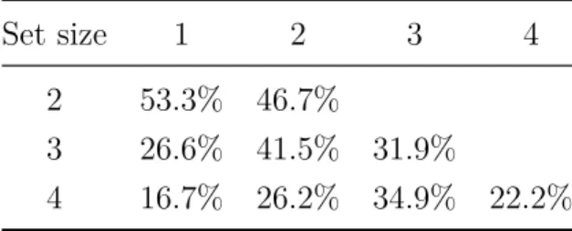
A first natural question is whether subjects chose non-singletons in ε-correspondences. Table1shows the size of the chosen sets depending on the size of the choice sets. Overall ε-correspondences, 59.7% of chosen sets are not singletons. Forcing subjects to choose only one alternative is a restriction in these cases. Only 8.2% of all ε-correspondences are choice functions. That is, subjects chose singletons in all choice sets. 3% of the subjects always chose as if I have forced them to choose singletons, that is, all their ε-correspondences are always made of singletons. For these subjects, eliciting a choice function is not a restriction.
Table 1also shows that the size of the chosen sets grows relatively faster than the size of the choice sets. For instance, the ratio of chosen sets of size one over chosen sets of size two decreases when the size of the choice set increases. One explanation for this phenomenon might be that choosing from larger sets is more complicated than choosing from smaller sets. I study menu-dependent – i.e., set-dependent – choice in Section 4.4.
Table 1: Proportion of chosen sets of different sizes for all ε-correspondences. Horizontally are the size of the chosen sets and vertically of the choice sets.
Set size 1 2 3 4
2 53.3% 46.7%
3 26.6% 41.5% 31.9%
4 16.7% 26.2% 34.9% 22.2%
The incentive to choose more than one alternative introduced by pay-for-certainty is one driver of non-singleton choice, but not the only one. Table2shows that even with no payments, subjects do not always choose singletons. The introduction of the additional payment has a non-linear effect on choices: a small gain significantly changes the aggregate proportion of singletons chosen, but small variations inside the gain domains do not. There is at least two possible explanation for this phenomenon. The first is the salience of even minimal monetary gains in experiments. The second is that very few subjects have a weak strict preference. The jump between no and low gains are due
to subjects who, when indifferent between two alternatives and faced with no gains, did not select all their maximal alternatives. When incentivized to choose all the maximal alternatives, they did so. The high gain is then not enough for them to bundle other alternatives with their maximal ones. I cannot disentangle the two explanations in the experiment. This aggregate behavior is consistent with increasing chosen set but is incompatible with the full identification of the choice correspondence for all subjects.
Table 2: Proportion of singletons chosen at different payments, depending on the size of the choice set. Differences between no gains and positive gains are significant. Differences between low and high gains are not.
Choice set size No Low High
2 65.6% 47.3% 46.5%
3 39.9% 20.5% 18.6%
4 27.0% 11.1% 11.6%
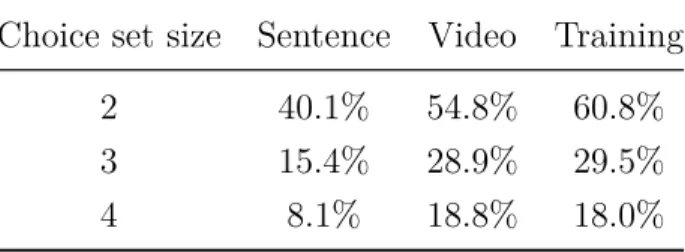
Table3shows another driver of non-singleton choice: lack of information. The proportion of single-tons chosen grows when the information on the tasks is more precise. The additional information provided by the video has a substantial effect on the choice of singletons. The additional infor-mation provided by the training is not as valuable for subjects, judging by the small additional proportion of singletons chosen.
Table 3: Proportion of chosen sets that are singletons, depending on the information and the size of the choice set.
Choice set size Sentence Video Training
2 40.1% 54.8% 60.8%
3 15.4% 28.9% 29.5%
4 8.1% 18.8% 18.0%
The non-singleton choice is a robust finding in the experiment. It persists even when providing better information on the alternatives or looking only at no gain of choosing more alternatives.
3.2
Increasing Chosen Sets
I have shown in Section 1 that increasing chosen set is key to assess the validity of the pay-for-certainty method. When a subject satisfies increasing chosen sets, I can at least partially identify her choice correspondence. Increasing chosen set is a within subjects across ε-correspondences consistency requirement. I have at most three pairs of additional payments for each subject: no
and low, no and high and low and high. To identify the choice correspondence, however, only the two pairs no and low payments and no and high payments matter. Because I am mainly interested in the identification of the choice correspondence, I only show in Table 4 results between no and low payments and between no and high payments.
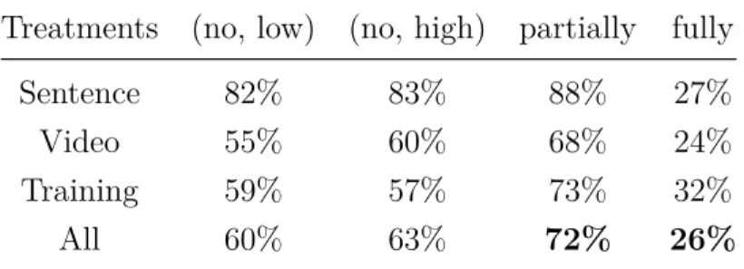
Table 4 shows that I identify the choice correspondence for 26% of the subjects, and partially identify it for 72% of them. Comparing the different treatments, increasing chosen set is overall significantly more satisfied in the sentence treatment than in the other two. It is due to a higher prevalence of fully indifferent subjects, as shown later in Section 5. These subjects always choose the whole set and therefore trivially satisfy increasing chosen sets. The training treatment provides better identification of the choice correspondence, but the difference is not significant.
Table 4: Proportion of subjects following increasing chosen set for different pairs of additional payments and different information.
Treatments (no, low) (no, high) partially fully
Sentence 82% 83% 88% 27%
Video 55% 60% 68% 24%
Training 59% 57% 73% 32%
All 60% 63% 72% 26%
The 28% of subjects who do not satisfy increasing chosen set violates the consistency requirement of the experiment. I cannot even partially identify their choice correspondence. Assessing the reason behind these violations is difficult. Maybe subjects chose at random – this is very unlikely, as will be shown in Section 4, maybe they are tired of making broadly similar choices and make some mistakes, and so on. One way to take into account the latter is to allow for some mistakes explicitly. If I allow subjects to violate increasing chosen sets in one set, the satisfaction rate rises to 85%, and if I allow for two mistakes, to 93%.
These numbers suggest that overall subjects understood the pay-for-certainty procedure and are generally consistent with the assumptions laid out in Section 1. Increasing chosen set is a robust property, satisfied with different treatments and almost always satisfied when I take into account the possibility of one or two mistakes.
From now on, I give the results for three different samples: • Choice correspondences, with 49 observations;
• Partially identified choice correspondences, with 137 observations. For simplicity and consis-tency, I use the choice obtained via pay-for-certainty with no payments for these. This choice is arbitrary; I could have presented the results with positive payments. The results are not significantly different. This sample also includes the sample of identified choice
correspon-dences.
• All ε-correspondences, 550 observations.
4
Reflexive, Complete, Transitive and Menu-Independent
Preferences, and Beyond
A decision maker behaves as if she has reflexive, transitive and complete preferences on X if and only if her choice correspondence satisfies the Weak Axiom of Revealed Preferences on 2X, as
shown by Arrow (1959). This result holds if and only if the choice correspondence is defined over the powerset, which is the case in my experiment. I borrow the formulation of WARP from Eliaz and Ok (2006).17
Axiom 4.1 (Weak Axiom of Revealed Preferences (WARP)). For any S ∈ 2X and y ∈ S, if there
exists an x∈ c(S) such that y ∈ c(T ) for some T ∈ 2X with x∈ T , then y ∈ c(S).
In words, if x is available in T and y is chosen, one may conclude that y is at least as good as x for the decision maker, and thus whenever x is chosen from a set S that contains y, so must y. The as if preference maximized by the decision maker is obtained using revealed preferences.
• x is weakly revealed preferred to y (denoted xRy) if and only if there is a set in which x is chosen, and y is available.
xRy ⇔ there exists S ∈ 2X, x∈ c(S), y ∈ S
• x is strictly revealed preferred to y (denoted xP y) if and only if there is a set in which x is chosen, and y is not.
xP y ⇔ there exists S ∈ 2X, x∈ c(S), y ∈ S\c(S)
• x is revealed indifferent to y (denoted xIy) if and only if there is a set in which both x and y are chosen.
xIy⇔ there exists S ∈ 2X, x∈ c(S), y ∈ c(S)
R, P and I are binary relations, that is, subsets of X2. When a decision maker satisfies WARP, P and I are a partition of R. In revealed preferences terminology, WARP states that it cannot be that both x is strictly revealed preferred to y and y is weakly revealed preferred to x, i.e., if xP y, then not yRx. It is easy to know which alternative is the best when WARP is satisfied, use the 17WARP has taken various names in the literature. It is Arrow (1959)’s Condition 4, Chernoff (1954)’s postulate 10 and Aleskerov, Bouyssou, and Monjardet (2007)’s Arrow’s Choice Axiom.
revealed preferences as the preferences of the decision maker.
4.1
WARP in Practice
Overall, 46% of ε-correspondences satisfy WARP and 57% of choice functions do.18 The difference
in satisfaction between choice functions and ε-correspondences is not significant. Only 19% of the subjects satisfy WARP for their 0, 1 and 12-correspondences together, whereas 25% never satisfy it. For subjects whose choice correspondence is partially or fully identified, the satisfaction of WARP rises to 58% and 98%. These numbers are lower than increasing chosen sets, indicating that some subjects are consistent across choice correspondences, but not within them.
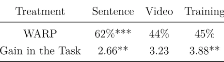
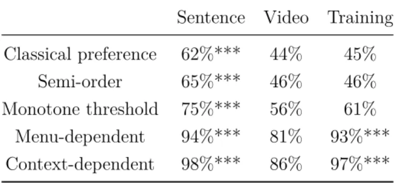
Table 5shows the satisfaction of WARP across the different treatments for ε-correspondences. The sentence treatment has the highest rate of satisfaction. As shown in Table 11 in Section 5, in the sentence treatment, subjects have more indifference relations. They choose more often the whole set, trivially satisfying WARP in the process. The information provided influences the quality of choice. Subjects earned more on average when they had more information, even though they satisfied WARP less.
Table 5: WARP and average gains by information, significance levels are assessed com-pared to the video treatment. For gains, the sentence and the training treatment are significantly different at the 1% level.
Treatment Sentence Video Training
WARP 62%*** 44% 45%
Gain in the Task 2.66** 3.23 3.88**
WARP and increasing chosen sets are two orthogonal consistency requirements, within and across
ε-correspondences. There is no reason a priori for them to be correlated, but they happen to be.
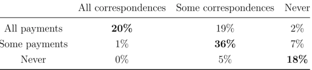
Each subject has two or three ε-correspondences. I can, therefore, assess for each subject whether some, all or none of their ε-correspondences satisfy WARP. Similarly, I can assess whether increasing chosen sets is satisfied for some, all or no additional payment pairs. Table6shows that these partial, full or absence of satisfaction of both axioms are correlated: 74% of the ε-correspondences are on the diagonal. Some subjects are more consistent than others, overall.
Few papers proceed to similar tests of WARP on experimental data. The setups can be largely different, but their results are not. They all show significant violations of WARP. Except Costa-Gomes et al. (2016), these paper all use choice functions to elicit preferences.
18One can wonder whether the different models I will present all along have explanatory power. The answer is yes, and I show in AppendixC.3.1 that none is trivially satisfied by a random choice correspondence or choice function. Incidentally, it proves that subjects have not chosen at random in my experiment.
Table 6: WARP and increasing chosen set.
All correspondences Some correspondences Never
All payments 20% 19% 2%
Some payments 1% 36% 7%
Never 0% 5% 18%
Bouacida and Martin (2017) have a section on experimental data and the satisfaction of WARP in an experiment that studies impatience. 47% of subjects satisfy WARP all the time, which is higher than the comparable figure of 19% found here, but they had only two choice functions per subjects, whereas here I have three choice correspondences, a more complex setup. On all ε-correspondences, the average rate of satisfaction of WARP is of 47% here and 64% in their experiment. Choi, Fisman, et al. (2007) found around 35% of subjects violating WARP for choices over risky assets. In the closely related large-scale field experiment of Choi, Kariv, et al. (2014), around 90% of subjects violate WARP for a similar choice task. My subject pool is in between their two pools, as shown in Appendix B.3. Costa-Gomes et al. (2016) found that 28% of observed choice correspondences satisfy WARP, a figure lower than here.19
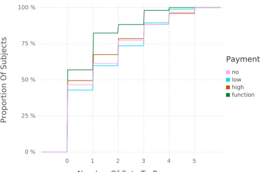
As I did with increasing chosen sets in Section 3.2, I can assess the severity of the violations of WARP. Figure1shows the minimal number of choice sets to remove in order to satisfy WARP, for different additional payments and the choice function.20 The number of sets to remove is different
between the choice functions and the ε-correspondences for the different payments at the 5% level, except for the high payment. As in the study of increasing chosen set, allowing for one or two mistakes, that is, removing one or two sets, increases the satisfaction of the axioms substantially. Indeed, 63% and 76% of ε-correspondences satisfy WARP with this relaxation. For choice functions, these numbers are respectively 82% and 88%.
4.2
Incomplete and Intransitive Indifference Preferences
It is possible to rationalize observed choice correspondences when WARP fails with relaxations of complete and transitive preferences.
First, I relax completeness, leading to partial orders (PO-rationalizability). The critique of the normative appeal of the completeness of preferences assumption dates back to Aumann (1962). Eliaz and Ok (2006) provide the first criterion for rationalizability of observed choices by incomplete preferences. Aleskerov, Bouyssou, and Monjardet (2007) provide an equivalent axiomatization.
19I give more details on this experiment in Section4.2.1.
20I averaged over all minimal combinations when different combinations of sets to remove are possible to rationalize observed choices.
Number Of Sets To Remove 0 1 2 3 4 5 no low high function Payment 0 % 25 % 50 % 75 % 100 % Proportion Of Subjects
Figure 1: CDF of the number of sets to remove in order to satisfy WARP.
Second, I relax transitivity of the indifference part. Intransitive indifference dates back at least to Armstrong (1939). These models are known as models of intransitive indifference or just-noticeable difference. I study two of the most common ones, semi orders (SO-rationalizability) from Luce (1956) and interval orders (IO-rationalizability) from Fishburn (1970).
I can investigate these models because I have identified choice correspondences. On choice func-tions, they rationalize the same observed choices, as explained in Appendix C.3.1. To the best of my knowledge, I am the first to study their empirical validity. There are other investigations of incomplete preferences in economics, but they rely on the identification of incompleteness with another phenomenon. For instance, Danan and Ziegelmeyer (2006) identify incomplete preferences with a preference for flexibility.
4.2.1 Incomplete Preferences
In addition to being normatively doubtful, Von Neumann and Morgenstern (1953) (p.19) have already criticized the validity of complete preferences from a positive standpoint:
It is conceivable – and may even in a way be more realistic – to allow for cases where the individual is neither able to state which of the two alternatives he prefers nor that they are equally desirable.
Aumann (1962) and Bewley (2002) point out that when choices are very hypothetical or very complex, it is not clear that an individual should have a definite preference over the alternatives.
Bewley (2002) and Ok (2002) are at the origin of representation theorems of incomplete preferences, in various contexts: certain, risky and ambiguous domains. A more thorough review is available in AppendixD.
There are many models of incomplete preferences in the literature, but there are comparatively very few studies on their empirical validity. Studying incomplete preferences is challenging, and to the best of my knowledge, only five experiments have investigated completeness, more or less directly: Danan and Ziegelmeyer (2006), Cettolin (2016), Sautua (2017), Qiu and Ong (2017) and Costa-Gomes et al. (2016). This small number should be contrasted with the large body of literature on completeness in psychology and management sciences (see Deparis (2013) for example), as well as the large body of evidence on violations of transitivity in economic contexts.
The main reason for the relative lack of experiment on the completeness axiom is conceptual. Jointly, revealed preferences and singleton choice forbid the exploration of the completeness axiom, as explained by Mandler (2005). First, assuming revealed preferences, an observer infers that chosen alternatives are preferred to unchosen ones. Second, singleton choice forces decision makers to choose precisely one alternative in the choice set. These two assumptions together impose what Mandler has called “observational completeness”. By definition, this setting assumes right away that chosen alternatives are comparable with unchosen ones, that is, preferences are complete. I solve this problem by using choice correspondences instead of choices functions, in contrast with all other experiments which use indirect mechanisms, except Costa-Gomes et al. (2016).
Eliaz and Ok (2006) introduces a weakening of WARP called the Weak Axiom of Revealed Non Inferiority (WARNI hereafter), with the interpretation that chosen alternatives are not worse than any other available alternative. This interpretation does not assume completeness of preferences anymore.
Axiom 4.2 (Weak Axiom of Revealed Non Inferiority (WARNI)). For a given alternative y in S, if for all the chosen alternatives in S, there exists a set T where x is in T and y is chosen in T , then
y must be chosen in S. This property should be true for all S and y.
for all S ∈ 2X, y ∈ S, if for all x ∈ c(S), there exists a T ∈ 2X, y ∈ c(T ), x ∈ T ⇒ y ∈ c(S)
WARNI states that if an alternative is not worse than all chosen alternatives, it must be chosen too. A choice correspondence satisfies WARNI if and only if it is rationalized by a reflexive and transitive strict preference relation – i.e., a partial order. Aleskerov, Bouyssou, and Monjardet (2007) give an equivalent axiomatization of rationalizability by a partial order, which is given in Appendix D.3.21 Their axiomatization is linked to Sen (1971)’s decomposition of WARP, rather