Oxygen and indicators of stress for marine life in multi-model global warming projections

HAL Id: hal-03113000

https://hal.archives-ouvertes.fr/hal-03113000

Submitted on 18 Jan 2021

HAL is a multi-disciplinary open access

archive for the deposit and dissemination of

sci-entific research documents, whether they are

pub-lished or not. The documents may come from

teaching and research institutions in France or

abroad, or from public or private research centers.

L’archive ouverte pluridisciplinaire HAL, est

destinée au dépôt et à la diffusion de documents

scientifiques de niveau recherche, publiés ou non,

émanant des établissements d’enseignement et de

recherche français ou étrangers, des laboratoires

publics ou privés.

multi-model global warming projections

V. Cocco, F. Joos, M. Steinacher, T. Frölicher, L. Bopp, J. Dunne, M. Gehlen,

C. Heinze, J. Orr, A. Oschlies, et al.

To cite this version:

V. Cocco, F. Joos, M. Steinacher, T. Frölicher, L. Bopp, et al.. Oxygen and indicators of stress for

marine life in multi-model global warming projections. Biogeosciences, European Geosciences Union,

2013, 10 (3), pp.1849-1868. �10.5194/bg-10-1849-2013�. �hal-03113000�

Biogeosciences, 10, 1849–1868, 2013 www.biogeosciences.net/10/1849/2013/ doi:10.5194/bg-10-1849-2013

© Author(s) 2013. CC Attribution 3.0 License.

EGU Journal Logos (RGB)

Advances in

Geosciences

Open Access

Natural Hazards

and Earth System

Sciences

Annales

Geophysicae

Nonlinear Processes

in Geophysics

Atmospheric

Chemistry

and Physics

Atmospheric

Chemistry

and Physics

Atmospheric

Measurement

Techniques

Atmospheric

Measurement

Techniques

Biogeosciences

Open Access Open Access

Biogeosciences

Discussions

Climate

of the Past

Open Access Open Access

Climate

of the Past

Discussions

Earth System

Dynamics

Open Access Open Access

Earth System

Dynamics

Geoscientific

Instrumentation

Methods and

Data Systems

Open Access

_{Geoscientific}

Instrumentation

Methods and

Data Systems

Geoscientific

Model Development

Open Access Open Access

Geoscientific

Model Development

Hydrology and

Earth System

Sciences

Hydrology and

Earth System

Sciences

Ocean Science

Open Access Open Access

Ocean Science

Discussions

Solid Earth

Open Access Open Access

Solid Earth

Discussions

The Cryosphere

Open Access Open Access

The Cryosphere

Natural Hazards

and Earth System

Sciences

Open Access

Discussions

Oxygen and indicators of stress for marine life in multi-model global

warming projections

V. Cocco1,2, F. Joos1,2, M. Steinacher1,2, T. L. Fr¨olicher3, L. Bopp4, J. Dunne5, M. Gehlen4, C. Heinze6,7,8, J. Orr4,

A. Oschlies9, B. Schneider10, J. Segschneider11, and J. Tjiputra6,7,8

1_{Climate and Environmental Physics, Physics Institute, University of Bern, Sidlerstrasse 5, 3012 Bern, Switzerland} 2_{Oeschger Centre for Climate Change Research, University of Bern, Z¨ahringerstrasse 25, 3012 Bern, Switzerland}

3_{Atmospheric and Oceanic Sciences Program, Princeton University, Sayre Hall, Forrestal Campus, Princeton, NJ 08544, USA} 4_{Laboratoire des Sciences du Climat et de l’Environnement (LSCE), L’Orme des Merisiers Bˆat. 712, 91191 Gif sur Yvette,} France

5_{Geophysical Fluid Dynamics Laboratory, NOAA, Princeton, New Jersey 08540, USA} 6_{Geophysical Institute, University of Bergen, All´egaten 70, 5007 Bergen, Norway}

7_{Bjerknes Centre for Climate Research, Bergen, Norway, All´egaten 55, 5007 Bergen, Norway} 8_{Uni Klima, Uni Research, All´egaten 55, 5007 Bergen, Norway}

9_{Helmholtz Centre for Ocean Research Kiel (GEOMAR), D¨usternbrooker Weg 20, 24105 Kiel, Germany} 10_{Institute of Geosciences, University of Kiel, Ludewig-Meyn-Str. 10, 24098 Kiel, Germany}

11_{Max-Planck-Institut f¨ur Meteorologie, Bundesstrasse 53, 20146 Hamburg, Germany}

Correspondence to: V. Cocco (cocco@climate.unibe.ch)

Received: 18 July 2012 – Published in Biogeosciences Discuss.: 13 August 2012 Revised: 22 February 2013 – Accepted: 27 February 2013 – Published: 19 March 2013

Abstract. Decadal-to-century scale trends for a range of

marine environmental variables in the upper mesopelagic layer (UML, 100–600 m) are investigated using results from seven Earth System Models forced by a high green-house gas emission scenario. The models as a class repre-sent the observation-based distribution of oxygen (O2) and carbon dioxide (CO2), albeit major mismatches between observation-based and simulated values remain for individ-ual models. By year 2100 all models project an increase in SST between 2◦C and 3◦C, and a decrease in the pH and in the saturation state of water with respect to calcium car-bonate minerals in the UML. A decrease in the total ocean inventory of dissolved oxygen by 2 % to 4 % is projected by the range of models. Projected O2 changes in the UML show a complex pattern with both increasing and decreas-ing trends reflectdecreas-ing the subtle balance of different compet-ing factors such as circulation, production, remineralization, and temperature changes. Projected changes in the total vol-ume of hypoxic and suboxic waters remain relatively small in all models. A widespread increase of CO2 in the UML is projected. The median of the CO2 distribution between

100 and 600m shifts from 0.1–0.2 mol m−3in year 1990 to 0.2–0.4 mol m−3 in year 2100, primarily as a result of the invasion of anthropogenic carbon from the atmosphere. The co-occurrence of changes in a range of environmental vari-ables indicates the need to further investigate their synergistic impacts on marine ecosystems and Earth System feedbacks.

1 Introduction

The ocean is undergoing physical and chemical changes in response to climate change caused by anthropogenic emissions of carbon dioxide (CO2) and other greenhouse gases. These changes include widespread ocean warming, alterations in the stratification, density structure, circulation and physical transport rates, and an increase in total car-bon content by air–sea CO2 uptake forcing the ocean to-wards more acidic conditions and altering acid–base rela-tionships (Bindoff et al., 2007). Oxygen (O2) and CO2 are involved in aerobic respiration where organic compounds and O2 are converted to CO2 and water. Global warming,

expanding hypoxia and higher CO2 levels represent physi-ological stresses for marine aerobic organisms that may act synergistically with ocean acidification (P¨ortner and Farrell, 2008).

The fugacity of carbon dioxide (f CO2) and oxygen (f O2) are two key thermodynamical variables for reporting the physiological state of aerobic marine animals (Hofmann et al., 2011; Seibel et al., 2012). The combined mechanisms of global CO2(and f CO2) increase and more local deoxy-genation (and f O2decrease) have just begun to be addressed (e.g., Paulmier et al., 2011; P¨ortner et al., 2011; Gruber, 2011; Mayol et al., 2012; Brewer and Peltzer, 2009) and need to be further investigated. Surprisingly, there is a lack of stud-ies that project the combined evolution of these variables un-der global warming and anthropogenic carbon emissions us-ing fully coupled Earth System Models.

The goals of this study are to provide multi-model es-timates of decadal-to-century scale trends in O2 and CO2 (together with f O2, f CO2, and other biologically rele-vant variables), as well as to identify underlying mecha-nisms using global warming simulations from six fully cou-pled atmosphere–ocean general circulation models and one model of intermediate complexity. The analysis focuses on how anthropogenic carbon emissions and climate change af-fect decadal-to-century scale changes in CO2and O2within the upper mesopelagic layer (UML, from 100 to 600 m of depth) under the SRES A2 high-emission scenario. The per-formance of current Earth System Models in representing observation-based variables is assessed. Using the range of models, uncertainties in the projected changes in different environmental variables that are potentially relevant for ma-rine life are explored. Thereby, the present analysis comple-ments available studies on temperature, pH or calcium car-bonate saturation state (i.e., the product of the concentrations of calcium ions and carbonate ion, divided by the apparent stoichiometric solubility product). Here we focus our anal-ysis on the UML because within this layer O2 is depleted the most as a consequence of the O2consumption associated with the remineralization of organic matter.

The concentrations of dissolved inorganic carbon (DIC, i.e., the sum of CO2, HCO−₃ and CO2−₃ concentrations) as well as f CO2are increasing in the surface ocean (0–100 m) and in the UML because a substantial fraction of the anthro-pogenic carbon emissions from fossil fuel burning and land use change is taken up by the ocean. Higher dissolved CO2 concentrations (i.e., the sum of CO2(aq)and H2CO3 concen-trations) induce, through acid–base equilibria, a decrease in pH and carbonate ion concentration, in turn reducing cal-cification in many calcareous organisms (Orr et al., 2005; Kroeker et al., 2010). Many physiological processes are sen-sitive to CO2 levels, and elevated CO2 concentrations may impose physiological stress on marine organisms more gen-erally (P¨ortner et al., 2008), even altering sensory responses and behavior of marine fishes (Nilsson et al., 2012). High CO2 may have detrimental effects on the survival, growth,

and physiology of marine animals and impair oxygen trans-port by lowering blood pH (P¨ortner et al., 2011).

Many observational (e.g., Pfeil et al., 2012; Watson et al., 2009; L¨uger et al., 2006) and modeling (e.g., Keller et al., 2012; Tjiputra et al., 2012; Thomas et al., 2008) studies are directed towards understanding the air–sea CO2 fluxes and uptake of anthropogenic carbon by the ocean. Recently, observational studies focused on upwelling regions (Mayol et al., 2012; Paulmier et al., 2011), typical low-O2–high-CO2 areas of particular vulnerability, where elevated f CO2levels represent a key threat connecting aerobic stress and calci-fication challenges. However, f CO2 and CO2are not state variables in ocean biogeochemical models and coupled Earth System Models, and their distribution below the surface layer has been studied poorly.

Observational studies indicate a mostly negative trend in the oxygen content over recent decades in different basins of the world’s ocean (Stramma et al., 2008; Chan et al., 2008; Whitney et al., 2007; Mecking et al., 2006; Emerson et al., 2004; Joos et al., 2003; Keeling et al., 2010; Takatani et al., 2012). A recent global-scale observational study (Helm et al., 2011) supports the evidence of a widespread ocean O2 de-crease between the 1970s and the 1990s. These authors, as well as Stramma et al. (2012), however, report also large ar-eas where O2has increased during recent decades.

The observed O2variations are relatively small and trends can therefore be difficult to detect, although they can re-sult in changes up to 50 % in the low-O2 regions. There is no consensus in considering anthropogenic global warming as the main driver of the observed O2 changes because of the relatively short and sparse observational records. Natu-ral variability may tend to mask the anthropogenically in-duced trends in dissolved O2, as suggested from both model-ing (Fr¨olicher et al., 2009) and observational (Meckmodel-ing et al., 2008; Deutsch et al., 2011) studies.

Despite the uncertainties about the last-decade trends, a long-term decrease in the oceanic O2inventory is expected under global warming and consistently simulated across a range of models (Sarmiento et al., 1998; Fr¨olicher et al., 2009; Plattner et al., 2002; Bopp et al., 2002). Surface warm-ing, lower sea surface O2concentration, enhanced stratifica-tion, reduced ventilation of the thermocline, and slowed ther-mohaline circulation tend to decrease the resupply of O2to the ocean interior, and to increase the residence time of water at depth, enhancing biological O2utilization.

Higher CO2levels may enhance O2consumption at depth because of the higher C/N ratio of the organic matter pro-duced at high CO2concentration, as shown in mesocosms ex-periments (Riebesell et al., 2007). As long as the O2/C ratio is not adjusted, this effect would lead to an expansion of the suboxic water volume in particular in the tropical oceans (Os-chlies et al., 2008). On the other hand, reduced upwelling of nutrient-rich waters may decrease export of biologically pro-duced organic carbon and the respiratory oxygen consump-tion in subsurface water. Many modeling studies identify

circulation and mixing changes as main drivers of the on-going and future O2decline (Fr¨olicher et al., 2009; Schmit-tner et al., 2008; Duteil and Oschlies, 2011; Bopp et al., 2002; Plattner et al., 2002). The observations reported by Helm et al. (2011) as well as earlier observation-based stud-ies (e.g., Emerson et al., 2001) also support this explanation. In the next section, simulations and experimental details are described. In the Appendix the model descriptions and additional plots are provided.

2 Methods

In this study we consider global warming simulations from seven Earth System Models including representations of ter-restrial and marine biogeochemistry of different complexi-ties. The models are forced with prescribed CO2emissions from reconstructions (1870–2000 AD) and a high-emission scenario, SRES A2 (2000–2100 AD). The Earth System Models represent the interactions between the physical cli-mate system, biogeochemical cycles, and marine ecosys-tems under global warming. Such interactions are included in global Earth System Models, but not in global ocean-only or high-resolution, eddy-resolving regional models. The strat-egy applied here is to analyze results from a broad suite of Earth System Models; the model spread in results provides a first indication of uncertainty.

The models are the IPSL-CM4-LOOP model from the In-stitut Pierre Simon Laplace (IPSL), the MPI-ESM Earth Sys-tem Model from the Max Planck Institute for Meteorology (MPIM), two versions of the Community Climate System Model (CSM1.4-carbon and CCSM3-BEC) from the Na-tional Center for Atmospheric Research, the Bergen Climate Model (BCM-C) from the University of Bergen and Bjerk-nes Centre for Climate Research, the Earth System Model from the Geophysical Fluid Dynamics Laboratory in Prince-ton, and the UVIC2-8 as used by the Helmholtz Centre for Ocean Research Kiel (GEOMAR). These models are referred to as IPSL, MPIM, CSM1.4, CCSM3, BCM-C, GFDL and UVIC2-8, respectively.

UVIC2-8 is an Earth System Model of intermediate complexity in which the ocean component is coupled to a single-level model of the atmosphere and a dynamic-thermodynamic sea ice component. The other models are fully coupled atmosphere–land–ocean carbon cycle general circulation models. The ocean model resolution ranges from about 1◦_×1◦_{(GFDL, up to 1/3}◦_{near the equator) to about}

3.6◦_×1–2◦_{(CCSM3, CSM1.4, and UVIC2-8). More details}

about the individual models are provided in Appendix A. The same simulations with IPSL, MPIM, CCSM3 and CSM1.4 models considered in this study are analyzed in Steinacher et al. (2010) to investigate the ability of the mod-els to represent the present spatio-temporal pattern of net pri-mary production and to project its future changes under the high-emission scenario SRES A2. Further details about these

four models and the experimental setup of the simulations considered here are provided in Steinacher et al. (2010). Schneider et al. (2008) present results for three (IPSL, MPIM, and CSM1.4) of the seven models used in this study. They provide detailed information on the performance of these three models under current climate conditions and com-pare modeled physical (temperature, salinity, mixed layer depth, meridional overturning, ENSO variability) and bio-logical (primary and export production, chlorophyll concen-tration) results with observation-based estimates. Roy et al. (2011) investigate the impacts of climate change and rising CO2on ocean carbon uptake with the simulations from IPSL, MPIM, CSM1.4 and BCM-C.

The models are forced by anthropogenic CO2emissions from fossil fuel burning and land use changes as recon-structed for the industrial period (from 1870 to 1999 AD) and following the SRES A2 emission scenario after 2000 AD. The CSM1.4, CCSM3 and the MPIM model also partly in-clude non-GHG forcings. Volcanic eruptions and changes in solar radiation over the historical period are also taken into account by CSM1.4 and CCSM3. The variables used in the analysis have been interpolated onto a common 1◦×1◦grid using a Gaussian weighted average of the data points within a radius of 4◦ with a mapping scale of 2◦. Control simula-tions in which atmospheric CO2 and other forcings are set to constant preindustrial levels are used to remove possible century scale model drifts for each grid point and for each month (Fr¨olicher et al., 2009). This procedure is applied to the three-dimensional field of temperature, salinity, oxygen, DIC, alkalinity and nutrients used in the following analysis.

As a point of reference we use annual GLODAP (Key et al., 2004) and World Ocean Atlas 2009 (WOA 09) (Lo-carnini et al., 2010; Antonov et al., 2010; Garcia et al., 2010a,b) gridded data sets for data–model comparisons. The gridded data sets provide structured information, extremely valuable in model–data comparisons and to estimate global properties.

2.1 CO2, f CO2and f O2

For this study, CO2and f CO2are computed using the stan-dard OCMIP carbonate chemistry routines (Orr et al., 2005; Steinacher et al., 2009) as a function of DIC, temperature, alkalinity, salinity, phosphate, and silicate (from observed or modeled quantities). f O2is computed following the Garcia and Gordon equation (Garcia and Gordon, 1992), in the ver-sion corrected by Sarmiento and Gruber (2006), as a function of dissolved O2, temperature and salinity (from observed or modeled fields). Changes in f CO2are attributed to changes in individual variables, i.e., to changes in DIC, temperature, alkalinity or salinity. This is done by keeping all input vari-ables except one at the 1870–1879 mean concentration in the carbonate chemistry computation. Similarly, changes in f O2 are attributed to changes in salinity, temperature, and O2.

The mechanisms responsible for the 21st century O2and DIC variations are investigated in more detail using CSM1.4 results and taking advantage of its relatively simple formula-tions for export production and remineralization. In CSM1.4 the stoichiometric O2to PO4ratio for production and rem-ineralization is fixed at −170. This allows splitting of the changes in O2(1O2) in individual components representing different drivers (see Fr¨olicher et al., 2009). 1O2gasreflects the contribution by air–sea gas exchange on the O2 concen-tration; this component reflects the influence of warming on the solubility of O2. 1O2bio is computed by multiplying the change in phosphate concentration with the O2to PO4 Red-field ratio; this reflects the influence from changes in the cy-cling of organic matter.

Similarly, the CSM1.4 changes in DIC due to marine pro-duction and remineralization of organic matter and calcite are linearly linked to variations in phosphate and alkalinity according to the fixed Redfield ratios (Plattner et al., 2001; Gruber and Sarmiento, 2002). This allows assignment of DIC changes (1DIC) to variations in the marine biological cycle (1DICbio) and in air–sea gas exchange (1DICgas) (Fr¨olicher and Joos, 2010). 1DICbiois given by the sum of two terms, representing the organic matter cycle and the calcium car-bonate cycle contributions. The difference between 1DIC and 1DICbiocan be assigned to 1DICgas.

2.2 Respiration index

Brewer and Peltzer (2009) proposed the “respiration index” (RI) as an indicator for estimating the physiological limits for deep-sea aerobic life. RI is a quantity linearly related to the available energy involved in the basic oxic respiration.

Generally, the limits to aerobic life in the ocean are defined in terms of a minimum dissolved O2concentration, which is typically set to 5 mmol m−3. Below this concentration mi-crobes turn to other electron acceptors as it becomes ineffi-cient to consume O2. However, by defining the limit in terms of oxygen only, the potential influence of CO2 on respira-tion is neglected. Brewer and Peltzer (2009), considering the basic oxic respiration equation Corg+O2→CO2and the re-lated Gibbs free energy (proportional to log10(f O2/f CO2)), proposed the RI.

Brewer and Peltzer (2009) proposed the RI with the fol-lowing thresholds, which can be used to map changing con-ditions: RI ≤ 0 corresponds to the thermodynamic aerobic limit (formal dead zone); the range 0 ≤ RI ≤ 0.4 has been proposed as “practical dead zone”; RI between 0.4 and 0.7 represents the practical limit of aerobic respiration; the inter-val from 0.7 to 1 may define an aerobic stress regime. The ac-tual limits will be, however, strongly species dependent and still need to be experimentally validated, as noted by Brewer and Peltzer.

Criticisms of the concept were raised and its practical usefulness has been questioned (Seibel et al., 2012; P¨ortner et al., 2011). The mechanisms of transport of O2 and CO2

between the environment and tissues are important controls influencing aerobic performance of large animals; a factor not included in the definition of RI. Acknowledging this lim-itation, we project changes in RI as another possible indicator of aerobic stress.

3 Results

3.1 Model evaluation

We start comparing model results with observation-based es-timates of the present-day annual mean distributions of f O2, O2, f CO2, DIC, and RI. First, the skill of the different mod-els in representing the observation-based fields for the world ocean between 100 and 600 m of depth is assessed by Tay-lor diagrams (TayTay-lor, 2001) (Fig. 1). The TayTay-lor diagrams allow us to visualize the correspondence between model re-sults and observation-based variables. The polar coordinates represent the correlation coefficient R (polar angle) and the normalized standard deviation σmodel/σobs(radius). In such a diagram the points corresponding to the observation-based variables would lie all at (R =1, σmodel/σobs=1). The Taylor diagrams of temperature, salinity, phosphate and mixed layer depth can be found in Roy et al. (2011) for the MPIM, IPSL, BCM-C, and CSM1.4 models. O2mean value and standard deviation (σ ) for WOA 09 and the models are listed in the table in Fig. 1a. BCM-C oxygen mean value and σ match the observations, GFDL has a slightly low mean value and the other models present in general too high mean values and too low σ . The correlation coefficient (R) for O2 and f O2 ranges for all models between 0.7 and 0.9, with a normal-ized standard deviation (σmodel/σobs) between 0.7 and 1.1 for both variables (Fig. 1). DIC shows very similar R values, and slightly higher normalized standard deviations (between 0.8 and 1.25).

The results for f CO2and RI are less satisfying. The cor-relation with the observation-based fields is lower than 0.6 for CCSM3 and CSM1.4 (for both variables) and for BCM-C (for f BCM-CO2). The normalized standard deviation for f CO2 lies between 1.1 (MPIM) and 1.9 (BCM-C), while for RI it ranges from 0.9 (IPSL) to 2.75 (CSM1.4 and CCSM3). The simplest model, UVIC2-8, produces the highest R values for all variables and normalized standard deviations between 0.9 and 1.2 for O2, f O2, DIC and RI. These results are in good agreement with the observation-based annual mean fields, compared with other models. This is true for the annual mean distribution; however, the situation for UVIC2-8 would look considerably worse considering the seasonal cycle.

Next, we compare the simulated and observation-based frequency distributions for O2and CO2within the UML. The frequency distributions allow us to assess whether the mod-els are able to represent the volume associated with a given concentration interval. Unlike the information in a Taylor diagram, the frequency distribution does not depend on the

0 0.5 1 1.5 0 0.2 0.4 0.6 0.8 1 1.2 1.4 1.6

Standard Deviation (norm.)

0 0.6 0.8 1 0.95 Correlation

[a]

[b]

Standard Deviation (norm.)

Standard Deviation (norm.)

0 _0.2 0.4 0.6 0.8 1 0.95 Correlation MPIM GFDL BCM-C CCSM3 CSM1.4 IPSL UVIC2-8 O2: Mean ± σ [mmol/m3_] WOA09 178±63 BCM-C 178±72 IPSL 192±50 UVIC2-8 201±61 CSM1.4 184±47 CCSM3 206±49 GFDL 174±72

Fig. 1. Taylor diagrams: correspondence between model results

(1990–1999 average) and observation-based (from GLODAP and

WOA 09, annual mean) f O2and O2(a), f CO2, RI, and DIC (b).

The polar coordinates represent the correlation coefficient R (polar

angle) and the normalized standard deviation σ_model/σobs(radius).

The results are relative to data between 100 and 600 m depth and are

weighted by the volume of each grid cell. Observed and modeled O₂

mean values and standard deviations (σ ) relative to the results of (a) are summarized in the table included in (a).

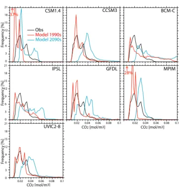
geographical location and is as such insensitive to a geo-graphical mismatch between observed and modeled water masses. Modeled and observation-based O2 and CO2 fre-quency distributions are shown in Figs. 2 and 3. Similarly to the observation-based O2frequency distribution, the mod-eled O2frequencies range between 0 and 400 mmol m−3, in-dicating the ability of the models to reproduce the correct range of variability of O2in the UML. The highest peak in

CSM1.4 UVIC2-8 GFDL IPSL BCM-C CCSM3 MPIM O2 [mmol/m3] O2 [mmol/m3] O2 [mmol/m3] Obs Model 1990s Model 2090s 100 200 300 400 Fr equenc y [%] Fr equenc y [%] Fr equenc y [%] 0 2 4 6 8 100 200 300 400 100 200 300 400 0 2 4 6 8 0 2 4 6 8

Fig. 2. O2frequency distribution in the UML (from 100 to 600 m

depth), obtained by sampling the volume fraction that falls within

20 mmol m−3intervals. Black line: observation-based distribution

(from GLODAP and WOA 09 gridded data). Red: 1990s mod-eled distribution (decadal mean). Blue: 2090s modmod-eled distribution (decadal mean).

the observations is at ∼ 300 mmol m−3. Most models tend to overestimate the magnitude of this peak and/or exhibit it be-tween 200 and 240 mmol m−3_.

The observation-based and modeled CO2values lie mostly between 0.01 and 0.06 mol m−3, with the highest peak at ∼ 0.02 mol m−3(Fig. 3). The magnitude of this peak is largely overestimated by CSM1.4, MPIM and, to a smaller extent, CCSM3 and GFDL. Modeled and observation-based vol-umes related to three O2concentration intervals in the low-O2range (Table 1) are analyzed next. For O2<80 mmol m−3 IPSL, UVIC2-8, CSM1.4, and CCSM3 underestimate the associated volume by a factor between 1.8 (UVIC2-8) and 3 (CSM1.4), compared to the data-based estimates. The other models overestimate it slightly (by a factor of 1.3 for the MPIM and 1.1 for the BCM-C). In the hypoxic range (O2<50 mmol m−3) the situation is analogous.

On the other hand, all models overestimate the wa-ter volume in the suboxic regime (O2<5 mmol m−3). The IPSL results are close to WOA 09 O2(respectively, 0.08 % and 0.05 % of the total volume of each data set). The other models simulate large discrepancies from the obser-vations, in particular GFDL and MPIM. As pointed out by Bianchi et al. (2012), these discrepancies in the suboxic regions could be only partially attributed to deficiencies of the gridded WOA O2 data set in representing the O2 minimum zones (OMZs), whose extent is considered by

Table 1. Observed and modeled present-day and 2090s (decadal average) volume of three water classes identified by different O₂regimes,

expressed in m3and in percent of the total oceanic volume. In the first line, the revised WOA 05 values from Bianchi et al. (2012) are listed.

Volume [1015m3] (% of the total)

1990s 2090s

O2<80 O2<50 O2<5 O2<80 O2<50 O2<5 mmol m−3 mmol m−3 mmol m−3 mmol m−3 mmol m−3 mmol m−3 Bianchi et al. 126 (8.58) 60.4 (4.33) 2.43 (0.16) – – – WOA 09 121 (8.27) 60.0 (4.10) 0.76 (0.05) – – – BCM-C 137 (10.4) 68.4 (5.20) 19.9 (1.51) 139 (10.6) 67.3 (5.12) 19.5 (1.48) IPSL 38.9 (2.98) 18.5 (1.42) 1.01 (0.08) 43.8 (3.36) 17.7 (1.36) 0.93 (0.07) UVIC2-8 67.9 (5.01) 32.9 (2.43) 4.91 (0.36) 67.8 (4.99) 32.8 (2.42) 4.91 (0.36) CSM1.4 33.3 (2.55) 18.1 (1.38) 5.44 (0.42) 35.8 (2.74) 18.7 (1.43) 5.39 (0.41) CCSM3 38.6 (2.94) 22.5 (1.71) 6.55 (0.50) 40.4 (3.07) 23.3 (1.77) 6.36 (0.48) GFDL 153 (10.7) 105 (7.35) 39.9 (2.79) 152 (10.6) 104 (7.28) 39.6 (2.77) MPIM 154 (11.3) 93.6 (6.87) 35.7 (2.26) 152 (11.1) 92.4 (6.78) 32.9 (2.42) 28% CSM1.4 UVIC2-8 GFDL IPSL BCM-C CCSM3 MPIM CO2 [mol/m3] CO2 [mol/m3] CO2 [mol/m3] Obs Model 1990s Model 2090s 0.02 0.04 0.06 0.08 0.1 Fr equenc y [%] Fr equenc y [%] Fr equenc y [%] 0 3 6 9 12 18 15 21 0 3 6 9 12 18 15 21 0 3 6 9 12 18 15 21 37% 0.02 0.04 0.06 0.08 0.1 0.02 0.04 0.06 0.08 0.1

Fig. 3. CO₂frequency distribution in the UML (from 100 to 600 m depth), obtained by sampling the volume fraction that falls within

0.02 mol m−3intervals. Black line: observation-based distribution

(from GLODAP and WOA 09 gridded data). Red: 1990s mod-eled distribution (decadal mean). Blue: 2090s modmod-eled distribution (decadal mean).

Bianchi et al. (2012) to be underestimated by a factor of three in the WOA 09 gridded data set. The spatial distributions of O2 and CO2 in the UML are compared with observa-tions using averaged values over the 100–600 m depth range (Figs. B1 and B2 in Appendix B). The CO2 pattern mir-rors the O2 distribution in observations and model results. This reflects the connection between the two variables via remineralization-production. High O2 values are associated

with low CO2values and vice versa. The observation-based O2(CO2) distribution exhibits generally high (low) values in the mid-latitude regions of both hemispheres and low (high) values in the tropics. Lowest O2and highest CO2values are observed in the Arabian Sea, the Bay of Bengal and the east-ern boundary upwelling systems of the Pacific and South At-lantic.

The models underestimate O2and overestimate CO2in the Atlantic eastern boundary upwelling regions, and, to some extent, in the Bay of Bengal, while they tend to overestimate O2and underestimate CO2in the Arabian Sea and in large areas of the Pacific – in particular in the North Pacific. These mismatches are linked to too low export production in the North Pacific and the Arabian Sea and too high export in the Bay of Bengal in the models (Steinacher et al., 2010). The relatively pronounced O2and CO2biases simulated by BCM-C in the Southern Ocean are related to the strong mix-ing process. Despite these deficiencies, the models represent many features of the observation-based CO2 and O2 fields between 100 and 600 meter depth, such as low O2 in the equatorial and eastern boundary upwelling systems, high O2 in the gyres and in the North Atlantic, and lower O2 in the North Pacific (Fig. B1 in Appendix B). Other reproduced fea-tures are the low CO2in the gyres and higher values in the equatorial and eastern boundary upwelling regions (Fig. B2 in Appendix B).

In conclusion, the comparison between model results and data-based estimates reveals that, while representing major large-scale features and global trends, the models suffer from considerable shortcomings in the representation of O2 and CO2. Regionally, large deviations in the CO2 in the UML compared to observations are not a surprise. Deviations in modeled DIC, alkalinity, temperature, and salinity all con-tribute to deviations in CO2and resulting errors can be large even if deviations in the four state variables (DIC, ALK, TEMP, and SALT) are modest as the carbonate chemistry is non-linear. In any case, the top-down forcing by rising

atmospheric CO2concentrations leads to rising DIC concen-trations (and f CO2), as found in the models and in observa-tions. Perhaps more problematic is the misrepresentation of the O2fields in the tropical UML. As the interest is to a large extent on the future evolution of low-oxygen regions, the challenge is in the correct representation of subtle changes in the balance between O2supply to the thermocline by physi-cal mixing and advection, and O2consumption by remineral-ization of organic material. Thus, we expect that projections of the evolution of low O2regions will vary among the mod-els and be affected by large uncertainties.

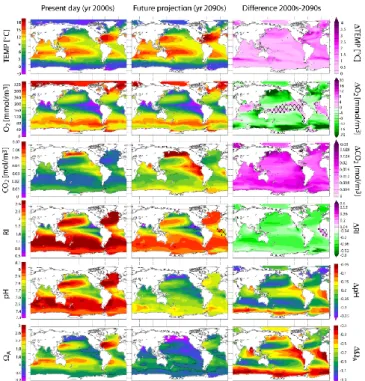
3.2 Projections

Figure 4 presents an overview of the current and projected distribution in the UML for a set of variables of poten-tial biological relevance: temperature, O2, CO2, RI, pH, and saturation state of water with respect to aragonite (A). A widespread warming of the UML is projected under the SRES A2 scenario with typical temperature changes over the 21st century of 1 to 2◦C. The 21st century changes in O2are less conspicuous on a global scale and no large expansion or contraction of thermocline regions with low O2 is pro-jected (variations are in general around ±10 mmol m−3). On the other hand, a large increase in CO2 is projected every-where in the UML. Concomitantly, a decrease in RI, pH, and

Ais evident in Fig. 4. The different models simulate a con-sistent increase in sea surface temperature, CO2uptake and O2outgassing (Fig. 5). Therefore, a widespread change in physical and chemical ocean properties is projected. Changes in O2, CO2, f O2, f CO2, and RI for the individual models are analyzed in more detail in the following sections.

3.2.1 Oxygen and f O2

A global decline in the oceanic dissolved oxygen inventory is projected by all models, with a 1870–2100 decrease be-tween 2 % and 4 % (for details about CSM1.4 see Fr¨olicher et al., 2009). The 21st century changes in the frequency dis-tribution of O2in the UML are modest (Fig. 2), with higher values becoming somewhat less abundant (in particular for MPIM, GFDL,UVIC2-8, and CCSM3). O2 changes in the UML (Fig. 6) show a complex pattern that reflects the in-fluence of different competing factors such as circulation, production, remineralization and temperature changes. The models simulate consistently, i.e., at least five of the seven models agree in sign, a decrease in O2 in the UML of the northern Pacific, the tropical and subtropical South Pacific, the Southern Ocean, the eastern part of the Indian Ocean and the subpolar North Atlantic. A relatively small increase in O2is consistently found in the multi-model average in the UML of the tropical oceans – including the eastern bound-ary upwelling system, the Caribbean Sea, western parts of the Indian Ocean, and the California upwelling region. The decrease is particularly pronounced (up to −60 mmol m−3)

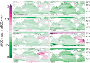
Fig. 4. Current and projected temperature, O2, CO2, RI, pH, and

A (100–600 m depth average). Observation-based fields from

GLODAP and WOA 09 are shown on the left. The second col-umn shows the projected 2090s distributions under the SRES A2 scenario, calculated as the sum of the observation-based fields and the 1990–2100 multi-model mean changes. The panels on the right represent the differences between the second and the first column. Hatched areas indicate where less than five out of seven models agree in the sign of the projected change. The contours represent

the thresholds RI = 1 and A=1.

in the northwestern Pacific in UVIC2-8, BCM-C, IPSL and GFDL. Modest changes are found in the UML around 40◦S, north of the equatorial Pacific, and in the subtropical At-lantic.

We next turn our attention to the low-O2regions and an-alyze whether they are projected to expand or to contract until 2100 under the SRES A2 forcing. Specifically, we address changes in the volume occupied with waters that hold less than 80 mmol m−3, less than 50 mmol m−3, and less than 5 mmol m−3 (Table 1 and Fig. 7). In Table 1 the projected 2090s (2090–2099 average) volume for the three low-O2 regimes and the different models is listed. While most models project a contraction of the suboxic waters (O2<5 mmol m−3), the model projections are not in agree-ment about the more oxygenated waters. Figure 7 illustrates the temporal evolution of the water volumes with low-O2, corresponding relatively to the 1870s (1870–1879 average) volume for each model and each low-O2class. By year 2100, four models project a modest expansion of the regions with O2concentration below 80 mmol m−3(Fig. 7a), in the range between 2 % (BCM-C) and 16 % (IPSL). UVIC2-8 does not

[b]

[a]

[c]

Fig. 5. Changes in sea surface temperature (a), air–sea CO₂flux

(b) and air–sea O2 flux (c) for the global ocean over the period

1860–2100.

exhibit relevant changes, and GFDL and MPIM show, re-spectively, a 2 % and 26 % reduction.

Projected changes in the volume with O2 concentra-tions below 50 mmol m−3(Fig. 7b) are smaller: two models (CCSM3, CSM1.4) project a 4.5 % volume increase, while the others project a decrease between 0.4 % (UVIC2-8) and 4.5 % (MPIM). For suboxic conditions (O2concentration be-low 5 mmol m−3_{, Fig. 7c), the volume is projected by most} models to contract slightly (up to −10 %). However, IPSL projects a 25 % contraction of the suboxic volume in the 2090s with respect to the condition in the 1870s.

Internal variability may mask part of the model–model dif-ferences, since we are analyzing single-mode simulations. Some models feature large interannual and decadal-scale variability in the volume evolution (especially IPSL). If such

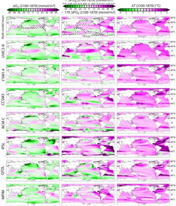
∆O2 (2100-1870) [mmol/m3] 0 -24 -12 12 -36 -48 -60 24 36 48 60 − ∆PO4 (2100-1870) [mmol/m3] 0 -0.14 -0.07 0.07 -0.21 -0.28 -0.35 0.14 0.21 0.28 0.35 ∆T (2100-1870) [°C] 0 -2 -1 1 -3 -4 2 3 4 CSM1.4 UVIC2-8 C CSM3 MPIM GFDL IPSL BCM-C 40°N 40°S 80°N 40°S 40°N 40°S 80°N 40°N 40°S 80°N 40°N 40°S 80°N 40°N 40°S 80°N 40°N 40°S 80°N 40°N 40°S 80°N 0° 0° 0° 0° 0° 0° 0° 0° M ulti-mo del mean 40°N 80°N − 170 ∆PO4 (2100-1870) [mmol/m3] 0 -24 -12 12 -36 -48 -60 24 36 48 60

Fig. 6. Projected changes in dissolved O2, PO4, and temperature (100–600 m depth average) under the SRES A2 scenario. Multi-model mean distributions are given in the first row; hatched areas indicate where less than five out of seven models agree in the sign of the projected change.

44

Fig. 6. Projected changes in f O2in the UML (100 to 600 m depth)

for the SRES A2 scenario. Changes are for 2100 relative to 1870. The multi-model mean is given in the upper left panel; hatched areas indicate where less than five out of seven models agree in the sign of the projected change.

a high variability is real, then it remains difficult to attribute current observation-based trends in low-O2regions to exter-nal natural or anthropogenic forcings. Conversely, UVIC2-8 does not show much variability, as it is an Earth System Model of intermediate complexity in which the ocean com-ponent is coupled to a single-level model of the atmosphere. As a representative example, we quantify for CSM1.4 the individual contribution of changes in salinity, temperature and O2to the change in the globally averaged depth profile of f O2 from 1870 to 2100 and for the SRES A2 scenario (Fig. 8a). Similar results are found for different ocean basins and the other models. f O2 decreases on global average on all subsurface layers by 10 to 25 matm. The largest decrease is found at around 250 m. At the surface f O2 increases by 7 matm on global average. The O2 concentration decreases in all depth layers on the global average. This decrease is the dominant driver of the decrease in f O2in the UML and the deep ocean. The influence of changes in O2 concentration is completely offset at the surface and, to some extent, in the thermocline by changes in temperature, while in the deep ocean the influence of temperature changes on f O2changes remains small. Changes in salinity generally have a small im-pact.

[b]

[a]

[c]

Fig. 7. Projected evolution of the global ocean volume occupied by (a) low oxygenated waters (O

<

80 mmolm

), (b) hypoxic waters (O

< 50 mmolm

) and (c) suboxic waters (O

< 5 mmolm

) for

the SRES A2 scenario and the range of models. Changes are given in percent of the 1870s volume,

relative to each low-O

class and each model.

45

Fig. 7. Projected evolution of the global ocean volume

oc-cupied by (a) low-oxygenated waters (O₂<80 mmol m−3),

(b) hypoxic waters (O2<50 mmol m−3) and (c) suboxic waters

(O2<5 mmol m−3) for the SRES A2 scenario and the range of

models. Changes are given in percent of the 1870s volume, relative

to each low-O2class and each model.

Next, we quantify the different mechanisms responsible for the changes in the O2 concentration following the pro-cedure described in the experimental design section and adopted from Fr¨olicher et al. (2009). Rising temperatures af-fect O2concentrations directly through the temperature de-pendence of gas solubility – estimated in previous studies being responsible for 25 % to 50 % of the total O2changes (Bopp et al., 2002; Plattner et al., 2002; Fr¨olicher et al., 2009). But warming induces also indirect effects, via strat-ification, circulation and soft-tissue pump alterations. As an illustration, we discuss average O2changes in the UML of the entire Atlantic Basin and in the Atlantic OMZs (i.e., O2

Fig. 8. Attribution to different drivers for changes (a) in f O2for the global ocean and (b) in dissolved

O2for the entire Atlantic (dashed lines) and for Atlantic hypoxic waters (O2< 50mmolm−3, solid

lines). Results are from CSM1.4 and represent differences between 1870s and 2090s. Colors in panel (a) indicate total changes in f O2(black), f O2changes due to changes in dissolved O2(green), in

temperature (red), and in salinity (blue). Colors in panel (b) indicate total O2changes (∆O2, black line),

changes due to the air-sea O2disequilibrium (∆O2gas, red), and to alterations in the cycling of organic

matter (∆O2bio, green).

46

Fig. 8. Attribution to different drivers for changes (a) in f O2for the

global ocean and (b) in dissolved O2for the entire Atlantic (dashed

lines) and for Atlantic hypoxic waters (O2<50 mmol m−3, solid

lines). Results are from CSM1.4 and represent differences between

1870s and 2090s. Colors in panel (a) indicate total changes in f O2

(black), f O₂ changes due to changes in dissolved O₂(green), in

temperature (red), and in salinity (blue). Colors in panel (b) indicate

total O2changes (1O2, black line), changes due to the air–sea O2

disequilibrium (1O2gas, red), and to alterations in the cycling of

organic matter (1O2bio, green).

smaller than 50 mmol m−3) as simulated by CSM1.4 over the period from 1870 to 2100 (Fig. 8b). The focus is on the Atlantic Basin because CSM1.4, compared to other models, simulates OMZs of limited extension in the Pacific.

In the Atlantic as a whole, O2concentrations decrease on average by around 7 mmol m−3_{in the upper 800 m. This} de-crease is driven by (1O2gas), i.e., by changes in solubility and air–sea fluxes not directly associated with changes in sat-uration concentration, whereas the reorganization of the bio-logical cycle leads to a decrease in phosphate and a related increase in O2(1O2bio) that partly offsets the decrease.

In the OMZs of the Atlantic, the O2concentration is pro-jected to slightly increase between 200 and 500 m depth (i.e., positive 1O2OMZ, Fig. 8b). At 250 m depth 1O2OMZshows the maximum increase of +3 mmol m−3. This increase re-sults from the slightly positive balance between a reduced O2consumption by remineralization and the reduced physi-cal flux of O2related to air–sea exchange.

A comparison of the spatial distribution of the changes in O2 and phosphate (Fig. 6) points to linkages between O2 changes in the thermocline and changes in the marine bi-ological cycle. In particular, a decrease in primary produc-tion, export of organic material and remineralization (see Steinacher et al., 2010) is linked to the projected O2(f O2) increase in the tropical Pacific and Atlantic, and in the Pa-cific eastern boundary upwelling systems. Regional changes in O2and phosphate in the thermocline differ among models similarly as for f O2. This reflects differences in how strat-ification and circulation is changing in the different models and how the balance between remineralization and physical tracer transport is altered in the thermocline. Such changes can reflect complex feedbacks and interactions between the physical and biogeochemical system, but their identification in the seven models is beyond the scope of this study.

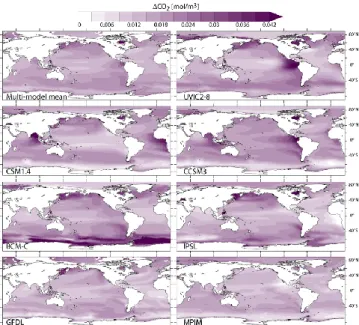
Fig. 9. Projected changes in CO2in the UML (100 to 600 m depth)

for the SRES A2 scenario. Changes are for 2090s relative to 1870s (decadal average). The multi-model mean is given in the upper left panel.

The seven models simulate consistently a warming UML under the SRES A2 scenario (Fig. 6), except in a few grid cells. Hence, in the UML the pattern of changes resulting from alteration in the biological cycle is shifted to smaller O2 concentration because of the decrease in O2solubility due to rising temperatures.

In conclusion, the net changes in O2depend on changes in the subtle balance between O2 supply by physical transport and O2consumption by remineralization. Both processes are linked as remineralization is primarily driven by the rate of export of organic matter, which itself depends sensitively on the physical transport of nutrients into the euphotic zone (Steinacher et al., 2010).

3.2.2 CO2and DIC

As expected under a high CO2 emission scenario, a widespread increase in CO2 in the UML (Fig. 9), as well as a shift towards higher values in the CO2 frequency distribution (Fig. 3), is projected by the end of the 21st century as a consequence of the atmospheric CO2 inva-sion. The highest peak in the frequency distribution, sit-uated at 0.1–0.2 mol m−3 _{in the 1990s, is found between} 0.2–0.4 mol m−3by the end of this century. CO2is projected to increase by up to 0.045 mol m−3 and large changes are simulated in the Atlantic and Pacific eastern boundary up-welling systems, in the Bay of Bengal (CSM1.4 and CCSM3) and in the North Pacific (GFDL, IPSL, BCM-C).

The simulated increase in DIC in the UML (Fig. 10) re-veals the familiar pattern of high changes in the

intermedi-Fig. 10. Projected DIC changes in the UML (100 to 600 m depth)

and for 2090s relative to 1870s (decadal average). The multi-model mean is given in the upper left panel.

ate water masses around 40◦N and 40◦S and in the well-ventilated North Atlantic, and relatively small changes in the tropical upwelling regions and around Antarctica. This pat-tern in DIC change is consistent among the different models and also consistent with observation-based reconstructions for the historical period (Sabine et al., 2004). This increase in DIC is predominantly driven by the invasion of anthro-pogenic carbon from the atmosphere. Changes in DIC due to the reorganization of the marine biological pump can be ap-proximately quantified by multiplying the simulated changes in phosphate (Fig. 6) with the typical C : P Redfield ratio of 117 after Anderson and Sarmiento (1994) (a value in the mid-dle of the range given by Takahashi et al., 1985; Redfield et al., 1963). These changes are typically much smaller than the simulated DIC increase.

We attribute the f CO2 change to changes in DIC, tem-perature, ALK, and salinity, following the procedure de-scribed in the experimental design section (Fig. 11a, b). The

fCO2increase is predominantly driven by the uptake of an-thropogenic CO2 from the atmosphere. On global average, changes in f CO2in the UML as well as in the deep ocean are predominantly driven by the increase in DIC, with addi-tional contributions resulting from the warming thermocline and minor contributions from changes in alkalinity on the global scale. For example, for CSM1.4 (Fig. 11b) the f CO2 increase at the surface is ∼ 470 µatm of which 400 µatm are attributed to the change in DIC. At 230 m depth the total increase is ∼ 560 µatm; the effect of temperature changes (+30 µatm) is one order of magnitude smaller than the DIC contribution (+510 µatm). The contributions from changes in salinity, phosphate and silicate to changes in f CO2are neg-ligible on global average.

In addition to anthropogenic carbon uptake, the change in DIC is also partly attributed to the reorganization of the marine biological cycle. The total 1DIC for the

∆fCO2 [µatm] [a] ∆DIC [µmol/kg] [b] 140 120 100 80 60 40 20 0 -20 D epth [m] 2500 1500 500 3500 4500 480 400 320 240 160 80 0 560 ∆DICgas ∆DICbio ∆DIC ∆fCO2 TEMP ∆fCO2 tot ∆fCO2 DIC ∆fCO2 ALK

Fig. 11. Panel (a): depth profile of the f CO2changes (difference 2100–1870) in the global ocean for

CSM1.4. Attribution of global f CO2changes to different drivers: total f CO2change (black line),

f CO2changes due to DIC (red), alkalinity (blue), and temperature (green). Panel (b): depth profile

of the Atlantic DIC changes (difference 2100–1870) for CSM1.4. Attribution of Atlantic Ocean DIC changes to different drivers: total DIC changes (∆DIC, black line), DIC changes due to gas exchange (∆DICgas, red) and biological cycle (∆DICbio, green).

49

Fig. 11. (a) Depth profile of the f CO₂changes (difference 2100–

1870) in the global ocean for CSM1.4. Attribution of global f CO2

changes to different drivers: total f CO2change (black line), f CO2

changes due to DIC (red), alkalinity (blue), and temperature (green).

(b) Depth profile of the Atlantic DIC changes (difference 2100–

1870) for CSM1.4. Attribution of Atlantic Ocean DIC changes to different drivers: total DIC changes (1DIC, black line), DIC

changes due to gas exchange (1DICgas, red) and biological cycle

(1DICbio, green).

Fig. 12. Fraction of changes in f CO2that is directly attributable

to changes in DIC. Changes are for the UML (100 to 600 m depth) and for 2090s relative to 1870s (decadal average). The multi-model mean is given in the upper left panel.

period 1870–2100 is about +130 mmol m−3 at the surface (Fig. 11b).

A slightly more nuanced picture emerges when consid-ering the contribution by individual drivers to the f CO2 changes in the thermocline on a regional level. In Fig. 12 the ratio between the f CO2 change due to DIC changes (1f CO_2DIC) and the total f CO2change (1f CO2tot) for the different models is plotted. The 1f CO2DIC/1fCO2tot ratio is generally below one, with the exceptions of the Atlantic and Arctic oceans for IPSL, the Atlantic and Indian basins for GFDL and the North Atlantic for the two NCAR mod-els and BCM-C. This results from the compensating effect of alkalinity changes (negative 1f CO_2ALKvalues) in these regions. A er obic str ess RI OBS RI CCSM3 1870 RI CCSM3 2100 RI CCSM3 = log(fO2 2100 / fCO2 1870) Respiration Index D epth [m] 2000 1000 0 3000 4000 2.8 2.4 2.0 1.6 1.2 0.8 0.4

Fig. 13. Regionally-averaged (105–115◦_{W, 0–10}◦_{N) depth profile of the Respiration Index, RI, as}

simulated by CCSM3 for 1870 (red) and 2100 (green) and as computed from the WOA 09 and GLODAP gridded data (black). The blue line is calculated by using the preindustrial f CO2values from CCSM3

in combination with projected f O2; the difference between the blue and red line is the 1870–2100 RI

change that is attributable to changes in f O2.

51

Fig. 13. Regionally averaged (105–115◦W, 0–10◦N) depth profile of the respiration index, RI, as simulated by CCSM3 for 1870 (red) and 2100 (green) and as computed from the WOA 09 and GLODAP gridded data (black). The blue line is calculated by using the

prein-dustrial f CO2values from CCSM3 in combination with projected

fO2; the difference between the blue and red line is the 1870–2100

RI change that is attributable to changes in f O2.

In conclusion, all seven models consistently simulate an increase in f CO2in the UML. Some regional differences re-main among the models and are likely related to differences in the thermocline ventilation and its change with time. The

fCO2increase is predominately driven by the uptake of an-thropogenic CO2from the atmosphere.

3.2.3 Respiration index

The observation-based RI distribution in the UML (Fig. 4) reveals minima in the eastern tropical Pacific, in the Arabian Sea and in the Bay of Bengal as well as in the eastern up-welling region of the Atlantic and Pacific, while maximum values are found in the Arctic.

Typically, simulated RI in the UML is on average reduced by 0.2 to 0.6 units between 1870 and 2100 (Fig. B3 in Ap-pendix B).

The RI depth profile in the eastern tropical Pacific (105–115◦W and 0–10◦N) and for CCSM3 is analyzed as an illustrative example to demonstrate the influence of changes in f O2and f CO2on RI (Fig. 13). This region is projected to become part of a large low-RI area in CCSM3. At preindus-trial time, simulated RI is well above unity, taken as threshold for aerobic stress, at all depths. RI is projected to decline in the upper 1000 m and RI falls on average below unity be-tween 300 and 600 m until 2100 under the SRES A2 sce-nario. This decline is the result of both a decline in f O2and an increase in f CO2.

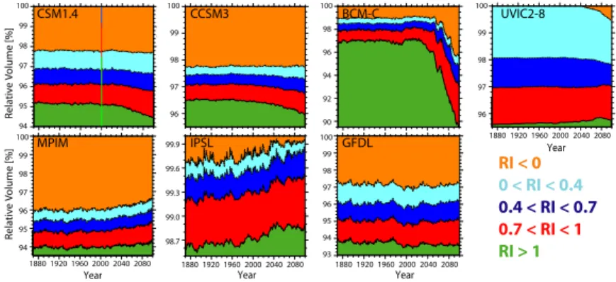
In Fig. 14 the evolution of the volume of five water classes over the period 1870–2100 is presented. Similarly to what is shown for the volume of low-oxygen waters, the models

RI < 0 0 < RI < 0.4 0.4 < RI < 0.7 0.7 < RI < 1 RI > 1 CCSM3 BCM-C MPIM IPSL GFDL UVIC2-8 Year 2040 1960 1880 1920 2000 2080 Year 2040 1960 1880 1920 2000 2080 Year 2040 1960 1880 1920 2000 2080 2040 1960 1880 1920 2000 2080 Rela tiv e V olume [%] 97 100 95 96 94 98 100 96 97 99 97 98 96 100 98 94 96 90 100 92 97 98 95 96 93 99 100 94 99.6 99.9 99.0 99.3 98.7 Year CSM1.4 Rela tiv e V olume [%] 100 96 98 94 95 97 99 99 98 99

Fig. 14. Projected changes in the volume of waters with a Respiration Index above (green) and below 1 (red to orange), calculated between 100 and 600 m of depth for the SRES A2 scenario. Volumes are given in percent of the oceanic volume in the 100–600 m depth range. The observation-based volume is represented in the first panel (vertical bars).

52

Fig. 14. Projected changes in the volume of waters with a respiration index above (green) and below 1 (red to orange), calculated between

100 and 600 m of depth for the SRES A2 scenario. Volumes are given in percent of the oceanic volume in the 100–600 m depth range. The observation-based volume is represented in the first panel (vertical bars).

project modest changes in the volume of water with RI < 0 (below 1 %). BCM-C represents an exception, projecting a 3 % expansion, mainly caused by a contraction in the vol-ume with RI > 1 (−3.5 %). UVIC2-8 exhibits a 0.6 % in-crease for water with RI < 0, while MPIM and IPSL project a 0.6 % and 0.3 % decrease, respectively. The other three models exhibit smaller changes. Diverging changes are found in the volume with RI > 1, which is projected to shrink by four of the seven models: CCSM3 (−0.4 %), CSM1.4 (−0.8 %), GFDL (−0.4 %) and BCM-C (−6 %). The other three models project an increase: +0.4 % for the MPIM,

+0.3 % for the IPSL and +0.2 % for the UVIC2-8, mainly driven by the hypoxic and suboxic waters contraction.

In conclusion, the models do not suggest a widespread ex-pansion of waters with RI below unity, consistent with small changes in the volume of hypoxic and suboxic waters. How-ever, RI declines in the UML in most regions due to the com-bined influence of rising f CO2and decreasing f O2levels.

4 Summary and discussion

In this study we have mapped the changes in a few potential stressors for aerobic organisms in the UML for a business-as-usual greenhouse gas emission scenario using a range of Earth System Models. The focus of this study is on the evolution of CO2, f CO2, O2, and f O2. Changes in these variables come in combination with changes in other envi-ronmental parameters, including a rise in temperature and hydrogen ion concentrations, and implied changes in the spe-ciation of trace metals and other acid–base relationships. These collective changes likely influence the performance and functioning of marine organisms in systematic and syn-ergistic ways. There exists a range of studies discussing pro-jections of pH and calcium carbonate saturation state under future anthropogenic carbon emission and global warming, and we refer the reader to the literature for further details (e.g., Kleypas et al., 1999; Orr et al., 2005; Steinacher et al., 2009; Fr¨olicher and Joos, 2010; Joos et al., 2011).

The Earth System Models represent the interactions be-tween the physical climate system, biogeochemical cy-cles, and marine ecosystems under global warming. The limitations in projecting O2 changes arise from the lim-ited understanding of the marine biological processes and the uncertainties about the future evolution of produc-tion/remineralization and marine ecosystem functions under rising CO2 (Oschlies et al., 2008; Steinacher et al., 2010). Changes in nutrient fluxes from land to coastal zones and in-creasing atmospheric nitrogen deposition (Duce et al., 2008) – which can result in local eutrophication and O2depletion – are not included. An intrinsic difficulty is the complexity and multitude of interactions and teleconnections. Gnanadesikan et al. (2012) analyze the O2changes in GFDL in detail. They identify an additional supply of O2along isopycnals that is fed by changes in convection and vertical mixing associated with salinification of the surface ocean off Chile. Their re-sults suggest that the simulated changes in the volume of suboxic water in climate models can depend sensitively on changes in the heat and salt balance in nearby convective re-gions and thus on the patterns of global warming and precip-itation minus evaporation. These authors examine also the pattern of the change in advective supply in GFDL and find that low-latitude O2 changes are driven by a decline in net upwelling across 1500 m with more influence from high-O2, low-nutrient, young surface waters and less from the older low-O2, high-nutrient deep waters.

For CSM1.4, Fr¨olicher et al. (2009) identify a significant warming of the ocean and a decreasing trend of ocean venti-lation, which both tend to lower oceanic O2, as well as a de-creasing trend in organic matter production, export and rem-ineralization, which tend to increase subsurface O2 and to decrease O2production at surface. These authors also high-light the role of variability related to climate modes such as the North Atlantic Oscillation and the Pacific Decadal Oscillation and to volcanic forcing. The models simulate consistently an increase in upper ocean temperature, carbon dioxide, and a decrease in pH and in the global O2inventory.

As expected under a high-emission scenario, a widespread increase of CO2 in the UML is projected. The increase in CO2 is primarily the direct result of the invasion of anthro-pogenic carbon from the atmosphere, and it is mainly respon-sible for the widespread decrease in RI outside low O2 re-gions. RI in the UML is on depth average reduced by 0.2 to 0.6 units.

Changes in dissolved O2(and f O2) are overall relatively small compared to the changes in CO2(and f CO2). The fre-quency distribution of O2in the UML is projected to change little over this century even for the high emission A2 sce-nario, a result that is consistent across the seven models. But projected changes in O2and dissolved O2in the UML are regionally of opposite sign. At least five out of seven models simulate in the UML a decrease in O2in the South-ern Ocean, in the northSouth-ern North Atlantic and North Pacific and in most of the subtropical Pacific and subtropical Indian Ocean, whereas O2 in the UML is projected to increase in the equatorial and subtropical Southeast Atlantic, off Cal-ifornia, in the Caribbean and tropical Indian Ocean in the multi-model average. Projected changes in the volume of hy-poxic waters (< 50 mmol m−3) are small and within ±7 % in the seven models. Similarly, projected changes in suboxic waters are small. Analogously to the evolution of the volume occupied by low-O2 waters, in general only small changes are projected for the volume of waters with a low RI.

The dominating mechanisms leading to changes in tem-perature and CO2versus those that affect O2in the UML are fundamentally different under rising anthropogenic green-house gas emissions. The decadal-to-century scale uptake of CO2 and heat by the ocean is driven “top down” by the in-crease in emissions of anthropogenic CO2 and greenhouse gases that cause atmospheric CO2 and radiative forcing to rise. The resulting perturbations in the air–sea temperature and CO2gradients cause a net flux of heat and CO2from the atmosphere to the ocean. The temperature and CO2content of the surface ocean increase and these perturbations are fur-ther penetrating the ocean by physical transport (advection, convection, diffusion). However, due to different uptake of CO2 by the land, individual models are forced by different atmospheric pCO2, even though emissions are identical.

The partial pressure or fugacity of O2in the surface ocean is, except for areas under sea ice, very close to the almost constant atmospheric O2 partial pressure. The typical time scale to equilibrate the well-mixed surface layer with at-mospheric O2 is roughly one month – much shorter than the multi-decadal ventilation time scales of the thermocline. Thus, in contrast to CO2 or pH and temperature, f O2 in the surface layer does hardly vary over multi-decadal time-scales. The long-term changes in f O2 and O2 within the thermocline reflect changes in the subtle balance between O2 supply from the surface layer to the thermocline, O2 con-sumption by the remineralization of organic matter within the thermocline, and advection and diffusion of low-O2 wa-ter masses from depth. In general, the models project an

increase in stratification and a reduction in surface-to-deep tracer exchange under global warming in mid- and low lat-itudes (Steinacher et al., 2010). In turn there is a decrease in O2advection to the thermocline, as well as nutrient sup-ply to the surface ocean, production, export, remineraliza-tion, and O2consumption within the thermocline. Reminer-alization rates are largely driven by the vertical flux of or-ganic particles that settle due to gravitation, whereas tracer transport has typically a large horizontal component, result-ing from advection and diffusion along the slopresult-ing layers of equal density. Not surprisingly then, the net balance of these opposing processes in terms of f O2and O2changes are re-gionally distinct.

We conclude that temperature, DIC and CO2 will con-tinue to rise, and pH and calcium carbonate saturation will continue to decrease in most regions in the thermocline. The link between these large-scale and substantial environmental changes and anthropogenic carbon emissions is firmly estab-lished and well understood. In contrast, changes in dissolved O2 resulting from global warming appear relatively small, regionally different, and uncertain. This calls for a distinc-tion of virtually certain ocean warming and acidificadistinc-tion ver-sus the postulated deoxygenation of thermocline waters in response to anthropogenic climate change. The challenge is in the observational detection as well as in correct represen-tation of the subtle changes in the balance between O2supply to the thermocline by physical mixing and advection, and O2 consumption by remineralization of organic material.

Appendix A Models

A1 IPSL

The IPSL-CM4-LOOP (IPSL) model consists of the Lab-oratoire de M´et´eorologie Dynamique atmospheric model (LMDZ-4) with a horizontal resolution about 3◦×3◦and 19 vertical levels (Hourdin et al., 2006), coupled to the OPA-8 ocean model with a horizontal resolution of 2◦×2◦·cos φ and 31 vertical levels and the LIM sea ice model (Madec et al., 1998). The terrestrial biosphere is represented by the global vegetation model ORCHIDEE (Krinner et al., 2005) and the marine carbon cycle is simulated by the PISCES model (Aumont et al., 2003). PISCES simulates the cycling of carbon, oxygen, and the major nutrients determining phy-toplankton growth (PO3−₄ , NO−₃, NH+₄, Si, Fe). The model has two phytoplankton size classes (small and large), rep-resenting nanophytoplankton and diatoms, as well as two zooplankton size classes (small and large), representing mi-crozooplankton and mesozooplankton. For all species the C : N : P ratios are assumed constant (122 : 16 : 1, Takahashi et al., 1985), while the internal ratios of Fe : C, Chl : C, and Si : C of phytoplankton are predicted by the model. Phyto-plankton growth is limited by the availability of nutrients and

light. For a more detailed description of the PISCES model see Aumont and Bopp (2006) and Gehlen et al. (2006). Fur-ther details and results from the fully coupled model simula-tion of the IPSL-CM4-LOOP model are given in Friedling-stein et al. (2006).

A2 MPIM

The Earth System Model employed for this study at the Max Planck Institute for Meteorology (MPIM) consists of the ECHAM5 (Roeckner et al., 2006) atmospheric model with 31 levels with the embedded JSBACH terrestrial bio-sphere model and the MPIOM physical ocean model, which includes a sea ice model (Marsland et al., 2003) and the Hamburg Ocean Carbon Cycle model HAMOCC5.1 ma-rine biogeochemistry model (Maier-Reimer, 1993; Six and Maier-Reimer, 1996; Maier-Reimer et al., 2005). The cou-pling of the marine and atmospheric model components, and in particular the carbon cycles, is achieved by using the OA-SIS coupler. HAMOCC5.1 is implemented into the MPIOM physical ocean model configuration using a curvilinear co-ordinate system with a 1.5◦ nominal resolution where the North Pole is placed over Greenland, thus providing rela-tively high horizontal resolution in the Nordic seas. The ver-tical resolution is 40 layers, with higher resolution in the up-per part of the water column (10 m at the surface to 13 m at 90 m). A detailed description of HAMOCC5.1 can be found in Maier-Reimer et al. (2005). The marine biogeo-chemical model HAMOCC5.1 is designed to address large-scale, long-term features of the marine carbon cycle, rather than to give a complete description of the marine ecosys-tem. Consequently, HAMOCC5.1 is a NPZD model with one phytoplankton group (implicitly divided into calcite (coccol-ithophorids) and opal (diatoms) producers and flagellates), one zooplankton species, and particulate and dissolved dead organic carbon pools. The model contains over 30 biogeo-chemical tracers, which include dissolved inorganic carbon, total alkalinity, oxygen, nitrate, phosphate, silicate, iron, phy-toplankton and zooplankton.

A3 CSM1.4

The physical core of the NCAR CSM1.4 carbon climate model (Doney et al., 2006; Fung et al., 2005) is a modi-fied version of the NCAR CSM1.4 coupled physical model, consisting of ocean, atmosphere, land and sea ice compo-nents integrated via a flux coupler without flux adjustments (Boville et al., 2001; Boville and Gent, 1998). The atmo-spheric model CCM3 is run with a horizontal resolution of 3.75◦and 18 levels in the vertical (Kiehl et al., 1998). The ocean model is the NCAR CSM Ocean Model (NCOM) with 25 levels in the vertical and a resolution of 3.6◦in longitude and 0.8◦to 1.8◦in latitude (Gent et al., 1998). The sea ice component model runs at the same resolution as the ocean model, and the land surface model runs at the same

resolu-tion as the atmospheric model. The CSM1.4-carbon model includes a derivate of the OCMIP-2 (Ocean Carbon Cycle Model Intercomparison Project Phase 2) ocean biogeochem-istry model (Najjar et al., 2007). In the ocean model, the bi-ological source–sink term has been changed from a nutrient restoring formulation to a prognostic formulation inspired by Maier-Reimer (1993). Biological production is modulated by temperature (T ), surface solar irradiance (I ), mixed layer depth (MLD), and macro- and micro-nutrients (PO3−₄ and iron). The C : P ratio is constant and set to 117 (Anderson and Sarmiento, 1994).

A4 CCSM3

The NCAR CCSM3 carbon is a coupled climate model that uses no flux correction (Collins et al., 2006b). The model components are the Community Atmosphere Model version 3 (CAM3, Collins et al., 2006a), the Community Land Model version 3 (CLM3, Dickson et al., 2006), the Parallel Ocean Program version 1.4 (POP1.4, Danabasoglu et al., 2006), and the Community Sea Ice Model (CSIM, Holland et al., 2006). In CCSM3 carbon, the land model is on the same horizontal grid as CAM3 (T31) and the sea ice model shares the same horizontal grid as the ocean model (gx3v5). Overall, CCSM3 carbon includes improvements in the parametrization of the physics as well as the biogeochemical cycles compared to earlier NCAR model versions (e.g., NCAR CSM1.4-carbon). New treatments of cloud processes, aerosol radiative forcing, land–atmosphere fluxes, ocean mixed layer processes, and sea ice dynamics are included. The CCSM3 Biogeochemi-cal Elemental Cycling (BEC) model includes several phy-toplankton functional groups, one zooplankton group, semi-labile dissolved organic matter, and sinking particles (Moore et al., 2004). Model–data skill metrics for the simulated ma-rine ecosystem in uncoupled ocean experiments are reported in Doney et al. (2009). The BEC includes explicit cycling of C, N, P, Fe, Si, O and alkalinity. Phytoplankton functional groups include diatoms, diazotrophs, picoplankton, and coc-colithophores. Phytoplankton Fe/C, Chl/C, and Si/C ratios adjust dynamically to ambient nutrient and light, while the C/N/P ratios are fixed within each group (Moore et al., 2004). The CCSM3 ocean circulation model is a coarse resolution version of the Parallel Ocean Program (POP) model with longitudinal resolution of 3.6 degrees and a variable latitu-dinal resolution from 1–2◦. There are 25 vertical levels with eight levels in the upper 103 m (Smith and Gent, 2004; Yea-ger et al., 2006).

A5 BCM-C

The Bergen Earth System Model coupled with terrestrial and oceanic carbon cycle models (BCM-C) is described in detail in Tjiputra et al. (2010), where regional climate–carbon cycle feedbacks are assessed. The physical ocean part of the BCM-C model is based on the Miami Isopycnic BCM-Coordinate Ocean