
HAL Id: hal-02946314
https://hal.archives-ouvertes.fr/hal-02946314
Submitted on 8 Oct 2020
HAL is a multi-disciplinary open access
archive for the deposit and dissemination of
sci-entific research documents, whether they are
pub-lished or not. The documents may come from
teaching and research institutions in France or
abroad, or from public or private research centers.
L’archive ouverte pluridisciplinaire HAL, est
destinée au dépôt et à la diffusion de documents
scientifiques de niveau recherche, publiés ou non,
émanant des établissements d’enseignement et de
recherche français ou étrangers, des laboratoires
publics ou privés.
ensemble of atmospheric CO2 inversions
P. Peylin, R. Law, K. Gurney, F. Chevallier, A. Jacobson, T. Maki, Y. Niwa,
P. Patra, W. Peters, P. Rayner, et al.
To cite this version:
P. Peylin, R. Law, K. Gurney, F. Chevallier, A. Jacobson, et al.. Global atmospheric carbon budget:
results from an ensemble of atmospheric CO2 inversions. Biogeosciences, European Geosciences Union,
2013, 10 (10), pp.6699-6720. �10.5194/BG-10-6699-2013�. �hal-02946314�
www.biogeosciences.net/10/6699/2013/ doi:10.5194/bg-10-6699-2013
© Author(s) 2013. CC Attribution 3.0 License.
Biogeosciences
Global atmospheric carbon budget: results from an ensemble of
atmospheric CO
2
inversions
P. Peylin1, R. M. Law2, K. R. Gurney3, F. Chevallier1, A. R. Jacobson4, T. Maki5, Y. Niwa5, P. K. Patra6, W. Peters7, P. J. Rayner1,8, C. Rödenbeck9, I. T. van der Laan-Luijkx7, and X. Zhang3
1Laboratoire des Sciences du Climat et de l’Environnement, UMR8212, Gif sur Yvette, France
2Centre for Australian Weather and Climate Research, CSIRO Marine and Atmospheric Research, Aspendale, Australia 3School of Life Sciences/Global Institute of Sustainability, Arizona State University, Tempe, USA
4University of Colorado Boulder and NOAA Earth System Research Laboratory, Boulder, Colorado, USA 5Meteorological Research Institute, Tsukuba, Japan
6Research Institute for Global Change, JAMSTEC, Yokohama, Japan
7Dept. of Meteorology and Air Quality, Wageningen University, Wageningen, the Netherlands 8School of Earth Sciences, University of Melbourne, Parkville, Australia
9Max-Planck-Institute for Biogeochemistry, Jena, Germany
Correspondence to: P. Peylin ([email protected])
Received: 30 January 2013 – Published in Biogeosciences Discuss.: 15 March 2013 Revised: 4 August 2013 – Accepted: 12 September 2013 – Published: 24 October 2013
Abstract. Atmospheric CO2inversions estimate surface
car-bon fluxes from an optimal fit to atmospheric CO2
measure-ments, usually including prior constraints on the flux esti-mates. Eleven sets of carbon flux estimates are compared, generated by different inversions systems that vary in their inversions methods, choice of atmospheric data, transport model and prior information. The inversions were run for at least 5 yr in the period between 1990 and 2010. Mean fluxes for 2001–2004, seasonal cycles, interannual variabil-ity and trends are compared for the tropics and northern and southern extra-tropics, and separately for land and ocean. Some continental/basin-scale subdivisions are also consid-ered where the atmospheric network is denser. Four-year mean fluxes are reasonably consistent across inversions at global/latitudinal scale, with a large total (land plus ocean) carbon uptake in the north (−3.4 Pg C yr−1(±0.5 Pg C yr−1 standard deviation), with slightly more uptake over land than over ocean), a significant although more variable source over the tropics (1.6 ± 0.9 Pg C yr−1)and a compensatory sink of
similar magnitude in the south (−1.4 ± 0.5 Pg C yr−1)
corre-sponding mainly to an ocean sink. Largest differences across inversions occur in the balance between tropical land sources and southern land sinks. Interannual variability (IAV) in car-bon fluxes is larger for land than ocean regions (standard
de-viation around 1.06 versus 0.33 Pg C yr−1for the 1996–2007 period), with much higher consistency among the inver-sions for the land. While the tropical land explains most of the IAV (standard deviation ∼ 0.65 Pg C yr−1), the
north-ern and southnorth-ern land also contribute (standard deviation
∼0.39 Pg C yr−1). Most inversions tend to indicate an
in-crease of the northern land carbon uptake from late 1990s to 2008 (around 0.1 Pg C yr−1), predominantly in North Asia. The mean seasonal cycle appears to be well constrained by the atmospheric data over the northern land (at the continen-tal scale), but still highly dependent on the prior flux season-ality over the ocean. Finally we provide recommendations to interpret the regional fluxes, along with the uncertainty esti-mates.
1 Introduction: context and objectives
Atmospheric CO2 inversions offer a method by which to
estimate carbon exchange between the land/ocean and at-mosphere by utilizing atmospheric CO2 measurements, a
key observational component of the global carbon cycle (e.g. their observed temporal and spatial gradients). Atmo-spheric CO2 inversions have a relatively long history with
the first comprehensive efforts dating to the 1980s (Enting and Mansbridge, 1989; Tans et al., 1989). After over a decade of work by individual investigators, an intercomparison was attempted in the late 1990s (Gurney et al., 2002). This was driven, largely, by the fact that many of the individual at-mospheric CO2 inversion efforts were arriving at distinctly
different estimates of the land carbon sink (referred to ini-tially as the residual or “missing” sink, deduced from fossil fuel emission, atmospheric accumulation, and ocean uptake) and it was sensible to attempt an improved understanding of the uncertainties and biases inherent to the problem.
This intercomparison effort, called “Transcom”, included a number of experiments and sub-projects. Transcom re-mains a convenient title for a large community of inverse modelers who regularly gather, compare results, and per-form various types of intercomparisons (e.g. Law et al., 1996; Denning et al., 1999; Gurney et al., 2002, 2004; Baker et al., 2006; Law et al., 2008; Patra et al., 2011). The major Transcom inversion intercomparison used a common inver-sion method across different transport models (Gurney et al., 2002, 2003), based on a Bayesian synthesis inversion method with a spatial discretization of 11 land and 11 ocean regions (Rayner et al., 1999). Annual mean, seasonal cycle, and inter-annual variability of the flux were analysed at different stages during the project (Gurney et al., 2002, 2003, 2004; Baker et al., 2006) along with a number of sensitivity studies (Enge-len et al., 2002; Law et al., 2003; Maksyutov et al., 2003; Pa-tra et al., 2003; Yuen et al., 2005; PaPa-tra et al., 2006; Gurney et al., 2008). In the early 2000s, new inversion approaches emerged, with different choices for spatial/temporal flux res-olution, prior information, and observational constraints (Rö-denbeck et al., 2003; Peters et al., 2005; Peylin et al., 2005; Chevallier et al., 2005, Maki et al., 2010). However, no ex-haustive intercomparison has been performed between these recent estimates (i.e. from global to regional scales), apart from regional initiatives in Europe (Schulze et al., 2010) and North America (Hayes et al., 2012) and individual studies in-vestigating only specific aspects of the carbon balance (e.g., Ciais et al., 2010, for the Northern Hemisphere long-term mean fluxes).
In this context, the results presented here are the latest comprehensive intercomparison. This effort was launched with the RECCAP initiative (REgional Car-bon Cycle Assessment and Processes, Canadell et al., 2011) as part of the international Global Carbon Project (http://www.globalcarbonproject.org/reccap/). In this con-text, the objectives of the paper can be defined as follows:
– Gather CO2flux estimates from recent atmospheric
in-versions and describe the main methodological simi-larities and differences between the selected systems. – Compare the estimated posterior fluxes from the
se-lected inversions using common processing.
– Analyze the fluxes in terms of term mean, long-term trend, interannual variations and mean seasonal variations and synthesize the most robust features at varying spatial scales.
– Provide guidelines and recommendations for using the inversion fluxes at the scale used in the RECCAP re-gional studies.
The paper is divided into four main sections. In Sect. 2, in-verse modelling principles and general issues related to the problem of inverting CO2fluxes over the globe are provided.
Section 3 reviews the main characteristics of the selected set of inversions. In Sect. 4, the global to continental-scale flux estimates are compared and analyzed at different temporal scales. Finally, the last section discusses issues involved with interpreting inversion results at regional scale.
2 Inversion methodology
2.1 Principles of atmospheric inversion
Atmospheric CO2inversions estimate surface-to-atmosphere
carbon fluxes using atmospheric CO2 concentration
mea-surements (see for instance Enting, 2002). The objective is to use the information from the temporal and spatial CO2
gradients to constrain a priori estimates of the net carbon exchange at the earth surface, including the anthropogenic component that is prescribed in the system. The prior natural fluxes are usually derived from a terrestrial/ocean dynamical model that can range from a complex process-based model to a simple linear model as in Rödenbeck (2005). The link be-tween the surface fluxes to be optimized (or model state, x) and the observations is made through the use of an observa-tional operator, namely an atmospheric transport model (H ):
y = H (x) + r, (1)
where y is a vector of the model-predicted observed vari-ables (atmospheric CO2), and r represents errors associated with measurements, representativeness (i.e. scale differences between model and observed concentrations), and the trans-port model (Kaminski et al., 2001).
The separation of the problem into observational and prior-knowledge components allows one to explicitly min-imize the difference between the simulated and observed quantities (i.e. atmospheric concentration) in addition to min-imizing the difference between the optimized fluxes and “background” or “reference” values (i.e. a priori surface fluxes). This can be recast in Bayesian terms as the max-imization of the probability density function (PDF) of the state variables given observations. Assuming Gaussian error distributions, the maximum of the PDF corresponds to the
minimum of the objective function, J1,
J (x) = (x − xb)TB−1(x − xb) + (yobs−H (x))TR−1
(yobs−H (x)) , (2) where B is the covariance matrix for the background or ref-erence state variables and R is the covariance matrix for the observations. These covariance matrices can be interpreted as weighting functions determining the extent to which the solution is influenced by the atmospheric data versus prior knowledge.
Note that this process can also be thought of as a particular application of a more general problem, described variously as model-data fusion, parameter estimation or data assimilation (DA) (Evans and Stark, 2002; Tarantola, 2005; Raupach et al., 2005). Indeed, the theoretical underpinnings of the atmo-spheric inverse approach have seen wide application in many branches of geophysics, economics, and systems engineer-ing, to name a few. Recently, new atmospheric inverse ap-proaches have emerged with the objective of constraining di-rectly the parameters of a terrestrial/ocean dynamical model; they are usually referred as Carbon Cycle Data Assimilation Systems (CCDAS, Rayner et al., 2005).
2.2 Inversion methods: practical implementation 2.2.1 Optimization method
A variety of approaches can be employed in finding the val-ues of x that minimize the above-mentioned objective func-tion (Tarantola, 1987; Rodgers, 2000; Enting, 2002). Sequen-tial approaches, in which the optimization occurs at regular intervals in time, can be used with different classes of the Kalman filter (Kalman, 1960; Evensen, 2007). An alternative is to simultaneously fit all the observations in the study pe-riod, either using a variational scheme such as in operational weather forecasting (Courtier et al., 1994) or an analytical scheme (Tarantola, 1987) when the dimensions of the prob-lem are small enough to allow storage of the matrix in com-puter memory (and their algebraic inversion). If the model H is a linear operator H, the posterior information on x follows a Gaussian PDF with mean value xa, and error covariance matrix A that can be calculated at least with two equivalent expressions2:
xa=xb−AHTR−1(Hxb−y) = xb−BHT
(HBHT+R)−1(Hxb−y) (3)
A = (HTR−1H + B−1)−1=B − BHT(HBHT+R)−1HB (4) Alternatively, in the variational approach, xa, the minimum of J can be estimated through an iterative descent algorithm,
1Notation follows the convention defined by Ide et al. (1997). 2The two expressions rely on different sizes of the matrix to
in-vert.
using the gradient of J (∇J ) at each iteration. Such compu-tation usually employs the adjoint technique in the case of large problems (Errico, 1997) and implies that R and B can be inverted (either being diagonal or having specific prop-erties). In this approach the estimation of A (corresponding to the inverse of the Hessian of J ) becomes more difficult and only selected elements corresponding to target quantities (e.g., regional averages) are usually estimated (Rödenbeck, 2005; Chevallier et al., 2010).
The choice of a particular formulation is usually guided by practical considerations: analytical approaches can be used if the number of observations or unknown variables is less than a few thousands and if all H terms can be calculated, while a variational approach is used for problems with larger size. Note that variational/analytical methods have the advan-tage of all state variables being exposed to all observations at once, while specific algorithms of the Kalman filter may have the advantage of smaller computational demand.
In this study, we present a number of atmospheric CO2
in-versions that employ this general approach, with differences in the detailed specification, which will be given in the inver-sion description (Sect. 3).
2.2.2 Atmospheric CO2observations
Atmospheric surface CO2 observations are obtained from a
global network of more than 100 sites where CO2 is
mea-sured either continuously (∼ 50 sites), or via discrete flask air samples (weekly; ∼ 100 sites). The current network is part of an international effort that started 55 yr ago with a continuously growing number of sites. Most of the sites are currently incorporated into the GLOBALVIEW data product (GLOBALVIEW-CO2: Cooperative Atmospheric Data Inte-gration Project – Carbon Dioxide. NOAA ESRL, Boulder, Colorado (available at http://www.esrl.noaa.gov/gmd/ccgg/ globalview/)) and are also available through the World Data Center for Greenhouse Gases (WDCGG). However, even with current networks, the interiors of most continents, as well as key areas of the ocean (i.e. southern oceans), remain undersampled with only a few space stations. Until recently, most inversions used data primarily from remote stations with air masses representing large-scale sources and sinks; coastal or inland station records would be selected, e.g. by wind sector or time of day, to avoid the influence of local fluxes. For flask samples, this selection occurs by choosing the sampling time, often with removal of outliers when the data are processed. More recently, inversion studies mak-ing use of improvements in modelled atmospheric transport are making greater use of continuous records of atmospheric CO2. For continental sites, these are usually selected by time
of day when transport models are expected to perform bet-ter (e.g., well-mixed conditions around local noon). Finally, note that none of the inversions considered in this study use column-integrated CO2observations acquired from space (as
growing number of vertical CO2profiles (not yet assimilated
in the selected inversions) would be useful to independently check on the inverse results (Stephens et al., 2007), exploit-ing them is a task beyond the scope of this paper.
2.2.3 Prior information
As noted previously, prior fluxes (or flux covariations) and prior flux uncertainties are utilized to supplement the pri-mary constraint supplied by the observed CO2
concentra-tions. Prior fluxes are used to maintain a rational posterior result where CO2 observations are insufficient to constrain
the degrees of freedom endemic to the inversion setup. The use of prior fluxes, their space/time distribution and numer-ical magnitude has engendered much discussion and debate. It is worth noting that prior fluxes cannot be discussed sep-arately from the prior flux uncertainties, as the latter deter-mines to what extent the priors are relied upon to constrain the posterior flux estimates.
Different inversion system groups have chosen different prior fluxes and uncertainties. The general approach is to uti-lize prior fluxes that are based on either independent model or observed estimates, such as net carbon exchanges as estimated by terrestrial or oceanic biogeochemical models (TBM, OBM). Most TBMs rely on different process for-mulations and to varying degrees upon observations or ob-served drivers (e.g. radiation, temperature, precipitation) but the quality of estimates varies depending upon the region considered (Sitch et al., 2008) and this reveals the extent to which net carbon exchange remains a challenging quantity to model.
The anthropogenic CO2source to the atmosphere due to
the combustion of fossil fuel (coal, gas, oil, cement produc-tion) is the main perturbation to the carbon cycle. It is known within 5–10 % from energy statistics (Andres et al., 2011, 2012) at the global scale, but with large uncertainties on the space/time distribution, particularly in industrial regions. Ge-ographic patterns of fossil fuel CO2sources are needed as an
a priori ingredient in the inverse problem, due to their high spatial heterogeneity. Although uncertainties in those emis-sions may substantially impact the annual land flux estimates at the regional scale (Gurney et al., 2005; Peylin et al., 2011), most inversions prescribe fossil fuel CO2 fluxes and do not
account explicitly for their uncertainty. This is discussed in more detail in Sect. 3.3.
3 Participating inversion systems 3.1 Selected inversions
The LSCE Laboratory has been collecting carbon flux esti-mates from state-of-the-art inversions performed by groups around the world in an effort to construct a new atmospheric CO2inversion intercomparison. Since the Transcom 3
inver-sion intercomparison of the early 2000s (Gurney et al., 2002,
2004; Baker et al., 2006), little effort has been made to sys-tematically compare and synthesize the results of more recent inversions.
Within the Transcom community, LSCE proposed shar-ing inversion results. Unlike the earlier Transcom 3 in-version intercomparison, there are no prescribed priors or a priori uncertainties, no prescribed inverse method and no prescribed observational data set, such that the ensem-ble of runs encompasses a wide range of methodological choices by the individual inversion groups. The only tech-nical requirement was to separately provide the estimated land and ocean fluxes and the fossil fuel emissions. The re-sults of these inversions are currently displayed through a web-site (https://transcom.lsce.ipsl.fr to be migrated under http://webportals.ipsl.jussieu.fr/), and represent 14 different approaches.
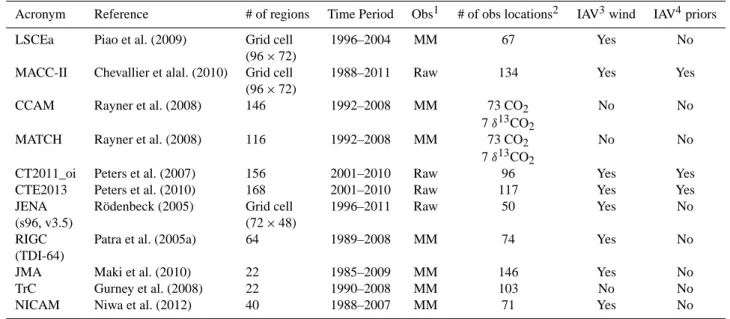
For the purpose of satisfying the RECCAP goals, eleven of the submissions to LSCE were selected (Table 1). The cri-teria used for the RECCAP synthesis was that the inversion results must span a time period of at least 5 yr (in order to ex-amine interannual variations). However a specific 5 yr period was not required. The specificities of the selected inversions and key associated references are briefly described in Sup-plement and summarised in Table 1. Note that inversion TrC is an ensemble mean of 13 inversions constructed using the inversion methodology of the Transcom 3 experiment (Gur-ney et al., 2002) and model submissions from that intercom-parison. We consider this as a single submission so that the results across inversions would not be biased towards a large number of inversions using a single methodology.
Note that for the selected systems we took the most recent flux estimates (early 2013) and that for five systems (JENA, MACC-II, NICAM, CT2011_oi, and CTE2013) older esti-mates have been used in the other RECCAP synthesis papers (released in 2011). We provide at the end of the Supplement a section describing the main differences between the old and new versions of the five systems as well as key figures with the old submissions (Figs. S9 to S12).
3.2 Main differences between the selected inversions The participating submissions reflect a range of choices for atmospheric observations, transport model, spatial and tem-poral flux resolution, prior fluxes, observation uncertainty and prior error assignment, and inverse method. We summa-rize here the differences among the selected inversions and the likely impact on the estimated CO2fluxes. Note that the
updated inversions do not result in any significant changes to the analysis presented here; the most notable difference is a general tendency to reduced spread across inversion results. 3.2.1 CO2observing networks
Previous work (Law et al., 2003; Patra et al., 2006; Gur-ney et al., 2008) has shown that the fluxes estimated in the
Table 1. Participating inversion systems and key attributes.
Acronym Reference # of regions Time Period Obs1 # of obs locations2 IAV3wind IAV4priors LSCEa Piao et al. (2009) Grid cell 1996–2004 MM 67 Yes No
(96 × 72)
MACC-II Chevallier et alal. (2010) Grid cell 1988–2011 Raw 134 Yes Yes (96 × 72)
CCAM Rayner et al. (2008) 146 1992–2008 MM 73 CO2 No No 7 δ13CO2
MATCH Rayner et al. (2008) 116 1992–2008 MM 73 CO2 No No 7 δ13CO2
CT2011_oi Peters et al. (2007) 156 2001–2010 Raw 96 Yes Yes CTE2013 Peters et al. (2010) 168 2001–2010 Raw 117 Yes Yes JENA Rödenbeck (2005) Grid cell 1996–2011 Raw 50 Yes No (s96, v3.5) (72 × 48)
RIGC Patra et al. (2005a) 64 1989–2008 MM 74 Yes No (TDI-64)
JMA Maki et al. (2010) 22 1985–2009 MM 146 Yes No TrC Gurney et al. (2008) 22 1990–2008 MM 103 No No NICAM Niwa et al. (2012) 40 1988–2007 MM 71 Yes No
1Observations used as monthly means (MM) or at sampling time (Raw).
2Number of measurement locations included in the inversion (some inversions use multiple records from a single location). 3Inversion accounts for interannually varying transport (Yes) or not (No).
4Inversion accounts for interannually varying prior fluxes (Yes) or not (No).
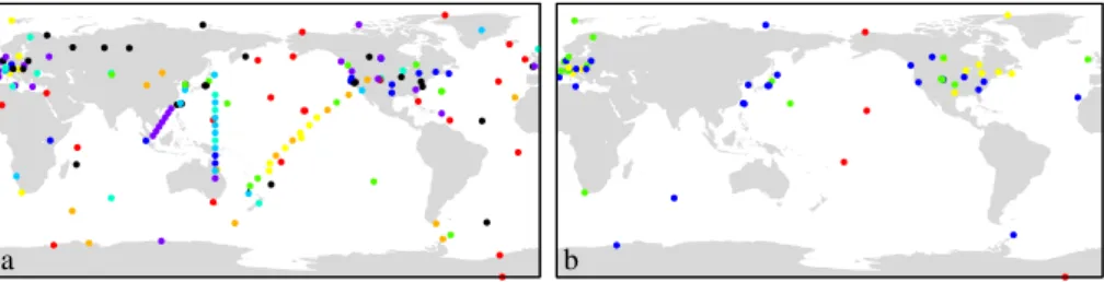
inverse approach can be very sensitive to the composition of the CO2observing network used (Fig. 1). This is particularly
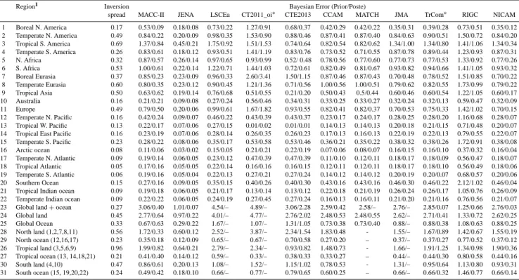
true for parts of the world where there are few observing sites; it is directly reflected in the estimated flux uncertain-ties (see Table 2) with larger values. Interannual variations (IAV) in the inversely estimated fluxes can also be sensitive to particular observing sites and the overall network com-position. Accurate quantification of the flux variability may be confounded by changes in the availability of observations through the estimation time period (Rödenbeck et al., 2003). Most inversions attempt to minimize this spurious variabil-ity by only using sites that are available for the full period of the inversion (LSCEa, JENA, RIGC), or by making use of the interpolated data in the GLOBALVIEW data product (CCAM, MATCH, TrC, NICAM). Note that the two Carbon-Tracker estimates (CT2011_oi, CTE2013) assimilate all data that were positively quality controlled by the inverse mod-elling team (i.e. removing outliers). The list of the observa-tion sites and data selecobserva-tion criteria used in each of the par-ticipating inversion systems can be found in the Supplement. Overall, the number of sites varies by a factor of almost three, i.e. between 50 (JENA) and 146 (JMA) (Table 1). Some in-versions directly assimilate raw data at the appropriate sam-pling time (weekly flasks or continuous record; MACC-II, CT2011_oi, CTE2013, JENA) while the other systems only use monthly mean values derived mainly from the GLOB-ALVIEW data product or from WDCGG (JMA). In general the GLOBALVIEW product uses data selected for clean-air conditions.
Finally, CCAM and MATCH additionally assimilate mea-surements of the 13C /12C isotopic ratio of CO
2 to further
constrain the partition between land and ocean carbon fluxes (Rayner et al., 2008). Note also that all groups have per-formed sensitivity tests with some stations added or left out. In this study we analyze only one variant of each inversion.
The inversion method requires an uncertainty to be as-signed to each CO2 observation. This provides a relative
weighting for each observation to determine the estimated fluxes. This uncertainty accounts for measurement errors as well as model errors (including representation error, i.e., the mismatch between the modelled spatial scale and the ob-served spatial scale). The model error is generally the largest contribution and it depends on each transport model’s charac-teristics. In general, all inversions place smaller uncertainties on remote ocean sites than on continental sites (see Supple-ment for the error range of each system).
3.2.2 Transport models
The different inversions used different transport models (see Supplement), except that CT2011_oi and CTE2013 both use the TM5 model but zoomed over either the US or both the US and Europe; LSCEa and MACC-II use two successive versions of the LMDZ model. Most of the participants drive their transport algorithms with interannually varying winds (Table 1), except for CCAM, MATCH, and TrC that utilize a single year of winds, which is repeated to achieve mul-tiyear results (a simplification that should be kept in mind when discussing the interannual flux variations). The value
a b
Fig. 1. Map of the site locations. Left shows all site locations used by any inversion with the color representing the number of inversions that
use that site: black: 1, purple: 2, dark blue: 3, light blue: 4, cyan: 5–6, green: 7–8, yellow: 9, orange: 10, red: 11; right: in situ sites that are used by up to 4 inversions at hourly or daily temporal resolution. Color indicates the number of inversions, 1 (blue), 2 (green), 3 (yellow), 4 (red).
of using interannually varying (IAV) transport was explored by Dargaville et al. (2000) and Rödenbeck et al. (2003), with the earlier study suggesting that utilizing IAV transport was less important than the later study.
3.2.3 Flux resolution
The number of adjustable degrees of freedom of the par-ticipating submissions varies considerably from the original 22 Transcom-3 land and ocean regions (JMA, TrC) to the transport model grid cells (LSCEa, MACC-II, JENA) (Ta-ble 1). Using a small number of regions with a prescribed prior flux pattern inside the regions imposes “hard” con-straints on the system (that may lead to “aggregation er-rors”; Kaminski et al., 2001), which potentially bias the observational error budget and the regional flux estimates. Hence, most inversions solve for increased numbers of re-gions (40–168). On the other hand, considering all grid cells as unknown fluxes relies heavily on additional “regulariza-tion constraints”. For instance, LSCEa, MACC-II, and JENA use spatial error correlations (matrix B, Eq. 2) for land and ocean pixels separately, decreasing with distance, to account for effective flux error correlations. However, they follow dif-ferent philosophies linked to the use of difdif-ferent prior models (Rödenbeck, 2005 for JENA; Chevallier et al., 2012 for both LSCEa and MACC-II cases) that lead to different correla-tion lengths: JENA uses larger correlacorrela-tion lengths (1000 km and 2000 km over land and ocean, respectively) compared to LSCEa and MACC-II (500 km and 1000 km, respectively) leading to smoother estimated fluxes from JENA compared to MACC-II (see for instance the mean annual flux distri-bution for each inversion in Supplement, Fig. S8 or under the web-site https://transcom.lsce.ipsl.fr). The regularization schemes based on correlation length scales significantly re-duce the number of degrees of freedom (dof, see Patil et al., 2001) in these grid-cell-based inversions to numbers compa-rable with but still higher than the region-based inversions. For instance, for the spatial domain, MACC-II has for land fluxes a number of dof (degree of freedom) close to 180 and JENA close to 60, while it is around 80 for CTE2013 and only 11 for TrC. All systems solve for monthly fluxes except
MACC-II, CT2011_oi, CTE2013, and JENA, which solve for weekly fluxes. These systems also use additional tem-poral error correlations for sub-monthly time steps (see Sup-plement). MACC-II also distinguishes between daytime and nighttime fluxes.
3.2.4 Prior flux information
The participating systems use diverse priors for biosphere, ocean and fossil fuel fluxes and prior errors (Supplement, Figs. S3 and S5, for prior land/ocean continental fluxes). For the land, all use net CO2 fluxes from terrestrial ecosystem
models with carbon pools brought to equilibrium and thus only weak annual mean carbon uptake (i.e., due to climate changes during the transient simulation), except JENA which uses a more conceptual approach (Rödenbeck et al., 2003). Moreover, only CT2011_oi and CTE2013 use land priors that vary from year to year, including fire disturbances to the land biosphere following the GFED2 approach (van der Werf et al., 2006). The associated prior errors vary between the systems with the LSCEa, MACC-II and JENA cases us-ing spatial error correlations (see above). In most inversions larger uncertainties are applied to land regions than ocean regions. For the sea–air exchange, most systems use clima-tological priors based on the pCO2 compilations of
Taka-hashi et al. (1999, 2002, 2009) except for CT2011_oi and CTE2013 which use priors based on ocean interior inversions (Jacobson et al., 2007), and JENA which combines different information (see Supplement for details).
The fossil fuel CO2 flux used as an imposed boundary
condition in each inversion contains differences amongst in-versions of up to ±8–9 % in annual global totals. There are different fossil fuel CO2 estimates available to the
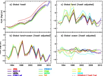
inver-sion community and different approaches to distributing the fluxes in space and time (sub-annually). Although most sys-tems used EDGAR, CDIAC or BP statistics, JENA has the largest global fossil fuel emissions while the others are gen-erally a little lower than the recent EDGAR v4.2 estimates (Fig. 2a). One reason for the discrepancy may be choices over which categories of emissions are included in the compila-tions used by any given inversion. Regionally, the differences
Fig. 2. Annual mean posterior flux of the individual
participat-ing inversions for (a) fossil fuel emission, (b) natural corrected” global total carbon exchange, (c) natural “fossil-fuel-corrected” total land and (d) natural “fossil-fuel-“fossil-fuel-corrected” total ocean fluxes.
can be much larger depending on the approach used by the different groups to scale a given gridded emission to global-or country-based total emission statistics (not shown). These differences will manifest as differences in the estimated nat-ural flux since the inversions only constrain the total (fos-sil + natural) flux from a region and assume no uncertainty in the fossil fuel estimate. Thus some of the natural flux ferences between inversions could be artefacts from the dif-ferences in the fossil fuel CO2 flux. We consider this as a
component of general model-to-model differences and a re-flection of actual uncertainty in fossil fuel emissions not yet accounted for in the individual inversions. However, to facil-itate comparisons between inversions, we have normalized the “natural” fluxes to account for fossil fuel differences (see Sect. 3.3 below).
3.2.5 Inverse method
Although all inversions use a Bayesian formalism with Gaus-sian errors for fluxes and data, the optimization is done by different algorithms. Many systems limit the number of un-knowns in order to be able to directly compute the optimal set of fluxes and their uncertainties, using a classical analyt-ical formulation (Tarantola, 1987; Rodgers, 2000). By con-trast, MACC-II and JENA use a 4-dimensional variational approach (4-D-var) derived from 4-D-var systems of numer-ical weather prediction (Courtier et al., 1994) to iteratively search for the optimal fluxes. These are efficient in the main estimation step, but need considerable extra iterations to de-rive elements of the posterior flux error covariance matrix or need to be combined with Monte Carlo methods (as is done in MACC-II). Finally, CT2011_oi and CTE2013 restrict the size of the problem using a Kalman smoother approach with
a 5-week moving window. In this approach the fluxes are ex-posed to only 5 weeks of atmospheric constraints, which re-sults in a slow spin-up of the system and may impact more significantly the estimated fluxes for the first year (excluded from the current analysis), than the other inversions. 3.3 Participant submission processing and flux
definition
Though the results reported by different participants were submitted at a variety of spatial resolutions, results were re-sampled onto a common 1◦×1◦grid (corresponding to the highest transport model resolution). This facilitated more direct comparisons between the inversion results. Once re-gridded, the results have been aggregated (i) to land and ocean regions consistent with the RECCAP regional divi-sions described in Canadell et al. (2011) and (ii) to larger scale totals (northern land, tropical ocean, etc) which are the focus of this paper.
A few technical complications arise with the aggregated totals. First, some submissions report solutions to the inverse problem at spatial scales larger than the RECCAP regional divisions. In this case, wherever possible, we have attempted to use any spatial information implicit in the inversion to aid in the down-sampling. For example, many inversions pre-scribe a flux distribution within a region when defining the basis function for each of the regions solved for. For exam-ple, TrC assumes land region fluxes are distributed according to CASA model estimates of net primary production (Ran-derson et al., 1997). Similar approaches were used by all in-version systems except LSCEa, MACC-II and JENA (being grid-cell-based inversions).
Second, each system has its own description of land/sea boundaries, based on the resolution of the transport model they use. After re-gridding, the application of common regional masks may not be compatible with the original land/sea mask of the system, which could bias the aggregated regional flux estimates. We minimize this problem by ex-tending the land (respectively the ocean) regional masks, pro-vided that the land and ocean fluxes were submitted as sep-arate variables. For each land region we included the neigh-boring pixels over adjacent ocean regions, and conversely for an ocean region.
3.3.1 Posterior flux definition
Because different inversion systems utilize different ap-proaches to define the prior fluxes and other boundary condi-tion informacondi-tion, some care must be taken to properly quan-tify what flux estimate is being compared across the inver-sion submisinver-sions. In this study, “natural” flux is defined as the total flux (all land, ocean, fossil) minus the fossil fuel flux used in the individual inversion submissions. Land use change related carbon fluxes, often accompanied by fires, are thus included in the natural land fluxes reported here.
However, as noted above, significant differences in pre-scribed fossil fuel emissions may complicate the inter-comparison of the estimated “natural” fluxes. In order to minimize this problem, we choose to “adjust” the natural land/ocean fluxes in order to account for these differences. We thus took the total surface-to-atmosphere gridded flux from each inversion and subtracted a common fossil fuel flux in order to obtain “fossil-corrected” natural land and ocean components (as in Schulze et al., 2010). For the reference fossil fuel emission, we took the recent annual gridded fluxes from EDGARv4.2. The underlying hypothesis is that the at-mospheric data constrain the total net surface flux so that extra fossil fuel emissions in a particular land region would be compensated by an increase of the natural land uptake of similar magnitude in that region, through the inversion. Note that such correction is only strictly valid at the global scale. At the regional scale, given the spatial and temporal pattern differences between “natural” and fossil fuel compo-nents in the inversion systems, such flux compensation may take place over a different region. This has been illustrated with the LSCEa system by Peylin et al. (2011). In this paper, we mainly discuss large-scale total fluxes (hemispheric or continental) where the correction should remain valid. How-ever, at the finer scale of the RECCAP regions, the fossil fuel correction should be handled with more care. Finally, most regional RECCAP analyses did not use the “fossil fuel correction” and several participating inversions revised their fossil fuel emission during the RECCAP exercise.
3.3.2 Flux processing
In this paper we mainly discuss the results aggregated in space and time. For the temporal scales we investigate sepa-rately the long-term mean, the inter-annual variations (IAV), the long-term trend, and the mean seasonal cycle.
For the long-term mean, since the inversions have been run for different time periods (the time period was not pre-scribed), identifying a common time period reduces the in-tercomparison time span for calculating multi-year means. We choose the 2001–2004 period included by all inversions, though this short period will still be considerably affected by interannual anomalies of these years. The IAV represent an-nual means with the individual inversion’s long-term means removed (in this case the long-term mean is defined over the entire submitted model time span). The long-term trend is ob-tained from the annual total anomalies (i.e. the IAV signal) by further smoothing these anomalies in time with a three-year moving window. The mean seasonal cycle is represented by 12 monthly values for each inversion. Each value is defined as the mean of all values of the considered month over the common period 2001–2004, minus the long-term mean over that period.
4 Global to continental-scale land and ocean results Here we present a series of results for each of the partici-pating inversions aggregated in space and time. We focus on latitudinally aggregated land and ocean totals as well as on a few continental regions (Supplement, Fig. S7). We show each of the submitting inversion posterior flux estimates (“natural” fossil-fuel-corrected flux). For the sake of clarity, we do not display the prior flux estimates. The prior fluxes for a few regions are given in the Supplement (Figs. S3 and S5) to en-able examination of the level of atmospheric constraint on the posterior fluxes versus that from prior information. 4.1 Annual total fluxes
4.1.1 Global totals
Figure 2a displays the global fossil fuel fluxes where signif-icant differences in the prescribed fossil fuel emissions are noteworthy. The JENA fossil fuel fluxes are larger than other inversions by ∼ 0.45 Pg C yr−1. Regionally, the differences are proportionally much larger (not shown); for instance over temperate Asia (Transcom region) the fossil fuel emis-sions range between 2.16 Pg C yr−1for CCAM/MATCH and 2.58 Pg C yr−1for JENA in 2004. Consequently, the JENA system requires greater global total carbon uptake by land and ocean to match the atmospheric CO2 growth
(Supple-ment Fig. S1 for the global land + ocean flux). These fossil fuel flux differences show up as an adjustment to the pos-terior natural fluxes estimated by each inversion system. As described in Sect. 3.3, we have thus corrected for these dif-ferences using EDGAR v4.2 emissions as a reference emis-sion. The natural land fluxes discussed below are “fossil-fuel-corrected” fluxes, unless noted otherwise.
The natural “fossil-fuel-corrected” global total carbon ex-change (land plus ocean, Fig. 2b) shows considerable agree-ment across the inversion systems because of the strong con-straint supplied by atmospheric CO2 measurements at the
global scale due to global tracer mass conservation. The year-to-year variations of the global total flux depicted in Fig. 2b reflect the variations in global atmospheric CO2
growth rate. As expected, they are robust across the differ-ent inversions, with large fluctuations associated with the oc-currence of El Niño and La Nina conditions. For instance, in 1998, and to a lesser extent in 1995 and 2003, El Niño conditions led to a reduction in carbon uptake by the land ecosystems. However, even with the “fossil fuel” correc-tion, the global annual totals show significant differences, up to 1 Pg C yr−1, among the different inversions in particular years. The differences are not systematic and reflect differ-ences between atmospheric transport mixing properties, es-pecially the mixing of surface fluxes to the upper atmosphere, as well as differences between inverse approaches and obser-vation data network. For example, both CarbonTracker sys-tems (CT2011_oi/CTE2013) provide similar fluxes in 2001
Fig. 3. Zonally integrated total carbon flux (natural land and ocean
plus fossil fuel) accumulated from the South to the North Poles for the individual participating inversions averaged over the 2001 to 2004 time period.
and 2002, although lower than all other inversions. Note fi-nally that the differences in the yearly mean may also reflect small differences in flux allocation between December and January (due to the “boxcar” average).
To further investigate the general mean behavior of the participating inversions, Fig. 3 displays the zonally grated total fluxes (natural land and ocean plus fossil), inte-grated from south to north for each inversion over the period 2001–2004. This zonally integrated cumulative flux reveals key characteristics of the inverse systems in general and in particular of the transport model used by each inversion. First one can notice that even for a 4 yr period (2001–2004) the to-tal net surface fluxes (values at the North Pole in Fig. 3) differ by up to 0.5 Pg C yr−1(see Sect. 4.2 below). More
interest-ingly, if we assume that all systems provide a reasonable fit to the atmospheric growth rate at all stations, the differences be-tween the shapes of the curve in Fig. 3 could reveal structural differences between the transport models and/or the longitu-dinal distribution of the total fluxes. For example, the much larger slope between 25◦S and 25◦N in RIGC, NICAM and MATCH may indicate that their transport models have dif-ferent atmospheric mixing over the tropics (stronger) than the other models or that their flux spatial distributions dif-fer. Large differences between the slopes of the integrated fluxes over the tropics (30◦S to 30◦N) reflect the poor at-mospheric constraint over this latitudinal band, while north of 30◦N the results are in much closer agreement. Overall, the zonally integrated flux diagnostic helps to differentiate and group the participating inversions. For instance, RIGC, NICAM and JMA and to a lesser extent MATCH and TrC systems have a different north to south flux behavior com-pared to the other systems.
4.1.2 Land and ocean totals
Figure also shows the partitioning between the global land and ocean aggregates (Fig. 2c and d). The major features are: – The natural land carbon exchange explains most of the total year-to-year flux variations with a strong agree-ment between all systems, but the annual long-term mean land fluxes differ significantly.
– The natural ocean carbon exchange does not present coherent year-to-year flux variations across the partic-ipating inversions, with mean annual flux differences similar to those of the land component (as required to give consistent total land plus ocean flux).
– The shift between the annual mean fluxes across all inversions are relatively constant through the investi-gated period, indicating that temporal variability is es-timated more consistently than longer-term flux aver-ages; although a subset of the inversion systems pro-vide more coherent results at the end of the period (af-ter 2002), potentially linked to the larger atmospheric network.
These results are discussed in more detail in the following sub-sections.
4.2 Long-term means
As explained in Sect. 3.3.2, the long-term means are defined for the 2001–2004 period, common to all inversions. Fig-ure 4 displays the total natural fluxes for the globe and three approximately latitudinal bands, as well as the partition be-tween the land and ocean. From the perspective of the long-term mean, the land and ocean (fossil-fuel-corrected) have similar values for global uptake, with the mean flux and stan-dard deviation across inversions giving around −1.32 ± 0.39 and −1.79 ± 0.30 Pg C yr−1, for land and ocean, respec-tively. The exceptions is the NICAM inversion, which gives the smallest land uptake (flux < −0.5 Pg C yr−1) compen-sated by the largest ocean sink (flux ∼ −2.5 Pg C yr−1). Note that for the JENA system, the old version used in some REC-CAP analyses had a different land/ocean flux partitioning, with an ocean flux close to −0.5 Pg C yr−1. The correlation between the time series of the annual total land fluxes and total ocean fluxes (for each inversion) ranges from −0.8 in RIGC to 0.8 in CT2011_oi with four systems having a corre-lation below 0.3 (JENA, MACC-II, LSCEa, and TrC). High positive or negative values may indicate the difficulties of the atmospheric inversion to separate land and ocean fluxes.
When analyzed in latitudinal bands, the mean “natu-ral” flux across the inversions results in a large total (land plus ocean) sink in the north (−3.4 ± 0.5 Pg C yr−1), a sig-nificant source over the tropics (1.6 ± 0.9 Pg C yr−1) and a compensatory sink of similar magnitude in the south
Fig. 4. Mean natural fluxes for the period 2001–2004 of the
indi-vidual participating inversion posterior fluxes. Shown here are total (first column), natural “fossil-fuel-corrected” land (second column) and natural ocean (third column) carbon exchange aggregated over the Globe (top row), the North (2nd row), the Tropics (3rd row) and the South (bottom row), with the three regions divided by ap-proximately 25◦N and 25◦S (but modified over land areas to keep regional estimates (e.g. northern Africa) in one region; see Fig. S7 in Supplement). Numbers in parentheses represent the mean flux and the standard deviation across all inversions.
(−1.4 ± 0.5 Pg C yr−1). If we take the median values to be less sensitive to outliers, we obtain similar uptake for the North and South (−3.4 and −1.2 Pg C yr−1, respectively) and a slightly lower tropical source of 1.1 Pg C yr−1. The spread between the different inversions at the scale of latitudinal bands is still relatively large. In the north, the MACC-II and LSCEa systems estimate the smallest total carbon up-take (−2.7 Pg C yr−1), while RIGC gives the largest uptake (−4.3 Pg C yr−1). Note that the RIGC behavior can be ex-plained by the stronger PBL trapping in the NIES/FRGCG transport model, as shown in Gurney et al. (2004). The spread among the inversions is much greater in the tropics, with a standard deviation close to 0.9 Pg C yr−1, reflecting, in part,
the low density of atmospheric stations in this region (Fig. 1). In the south, the spread obtained for the total flux is compa-rable to the north (σ values are close to 0.5 Pg C yr−1 for both north and south regions). Finally one should also notice that all inversions neglect the 3-D source of CO2 from the
oxidation of reduced carbon compounds in the atmosphere (i.e., source treated as a surface flux) and that such simpli-fication might bias the northern continental land uptake by
0.2 Pg C yr−1(too large an uptake) as discussed in
Sunthar-alingam et al. (2005).
Two groupings of inversion results arise in the latitudi-nal aggregate alatitudi-nalysis. JENA, LSCE, MACC-II, and the two CarbonTracker results (group 1) provide nearly identical car-bon uptake in the south (−1.2 ± 0.1 Pg C yr−1)and a carbon release between 0.8 and 1.0 Pg C yr−1in the tropics mostly from the ocean. MATCH, CCAM, TrC, and NICAM in-versions (group 2) give a much larger carbon release over the tropics, compensated by a larger uptake in the south and north. RIGC and JMA give moderate to large sources over the tropics but only a small southern carbon sink. It is not clear whether these differences can be attributed to methodological differences in the inversion, since the agree-ment within the two groups breaks down at continental scale, e.g. in the distribution of the tropical source between Africa, Asia and South America. However, several sources of sys-tematic differences could be envisaged.
With the exception of LSCEa, one difference between the group 1 and group 2 inversions is that group 1 inversions use the atmospheric data at their sampled times as opposed to monthly means. This should allow group 1 inversions to better represent baseline-selected data, whereas group 2 in-versions may be allowing baseline-selected data to influence nearby land regions, where no constraint exists in reality. This could result in more variable flux estimates for land re-gions across group 2 inversions than for group 1 inversions. A second possible source of differences is that group 1 cor-responds to inversions that solve for fluxes at the resolution of the transport model or for small ecosystem-based regions over land (both CT systems), with the exception of MATCH and CCAM inversions (group 2) that also solve for a large number of regions. Other potential sources of difference are not systematically associated with group 1 or 2: (i) the prior fluxes do not exhibit systematic differences between group 1 and 2, although TrC, MATCH, and CCAM impose a large prior deforestation flux over the tropics (∼ 1.5 Pg C yr−1; Supplement, Fig. S3), and (ii) there is no clear systematic differences in the transport characteristics between the two groups, in terms of wind field or spatial resolution.
Finally, the division of the total natural fluxes (fossil-fuel-corrected) from each latitude band into land and ocean com-ponents (second and third column of Fig. 4) shows that:
– In the north, the land natural sink appears to be twice as large as the ocean sink with a significant spread across the inversions, with the land contributing from around 50 % of the total for NICAM to 80 % of the total for RIGC. The group 1 inversions (the first five systems in each panel of Fig. 4) produce the lowest land sink, around −1.8 Pg C yr−1, while the other inversions esti-mate a much larger land sink, close to −2.5 Pg C yr−1. – In the tropics, all inversions tend to produce a simi-lar ocean carbon source of around 0.7 Pg C yr−1with a relatively small spread (σ = 0.2 Pg C yr−1). Such a
value does not significantly deviate from the prior ocean fluxes used by the inversions, mostly based on one of Takahashi et al. (1999, 2009) climatolo-gies (See Supplement, Fig. S5, with values between 0.5 and 0.9 Pg C yr−1for all inversions). On the other hand, the land natural carbon exchange shows a large spread across all participating inversions, with a mean positive flux to the atmosphere of 0.9 Pg C yr−1 but with a standard deviation that is of the same size, i.e. 0.9 Pg C yr−1. However, group 1 inversions present a much smaller land carbon source or a small land sink (flux between −0.05 and +0.46 Pg C yr−1). For these inversions, the tropical ecosystems store carbon at a rate that would compensate the emis-sions through deforestation, i.e., on the order of 1.4 Pg C yr−1(Houghton, 2008). Note that the net
de-forestation carbon flux is still highly uncertain as a large part of the total biomass burning flux comes from burning of savannah and grasslands, which sub-sequently regrow. Overall, the strong atmospheric ver-tical diffusivity in the tropics due to convection, com-bined with generally under-observed CO2distribution,
explain the larger inversion spread.
– In the south, all inversions produce a large ocean car-bon uptake, with a flux around −1.3 Pg C yr−1 and a relatively small spread. Note that the prior ocean flux ranged from −1.8 Pg C yr−1 (4 inversions) to
−1.1 Pg C yr−1(4 inversions) but that inversions start-ing with small or large priors span the full range of posterior flux estimates. Over land, the inversions do not agree on the sign of the natural flux, varying from
−0.6 to +0.5 Pg C yr−1.
Finally, we briefly investigate the long-term mean nat-ural fluxes within continental/basin-scale subdivisions of the Northern Hemisphere where the atmospheric network is denser: North America, Europe, North Asia, North At-lantic and the North Pacific (Fig. 5). The region bound-aries are shown in Supplement, Fig. S7. The three land regions show a significant carbon sink, with fluxes from
−0.4 Pg C yr−1 over Europe to −1.0 Pg C yr−1 over North Asia. A large spread among the inversions remains with standard deviations of up to 0.45 Pg C yr−1for each region. When differences in surface area are accounted for, Europe exhibits the greatest land uptake (−40 g C m−2yr−1) and North Asia the smallest (−26 g C m−2yr−1). For the two
ocean basins, the inversions estimate a sink with a flux of
−0.5 to −0.6 Pg C yr−1and a smaller spread than found on
the land (σ = 0.1–0.15 Pg C yr−1). This agreement partly re-flects the use of similar prior ocean fluxes in the inversions (see Sect. 3.2.4), with relatively tight errors compared to the land fluxes. The prior fluxes (Supplement, Fig. S5) vary be-tween −0.5 and −0.7 Pg C yr−1for both the North Atlantic and North Pacific. Expressed per surface unit, the estimated North Atlantic sink (−15 g C m−2yr−1)is 60 % larger than
the North Pacific one (−9 g C m−2yr−1). Overall, the
longi-tudinal breakdown of the total northern sink appears to be much more variable than the total flux itself. Statistically, adding the flux variances of the four regions, calculated from the spread of the 11 inversions, would lead to a standard deviation of the Northern Hemisphere total flux of roughly 0.8 Pg C yr−1, a value significantly larger than that calculated directly from the spread of the 11 Northern Hemisphere to-tals, 0.5 Pg C yr−1(Fig. 4).
4.3 Interannual variability
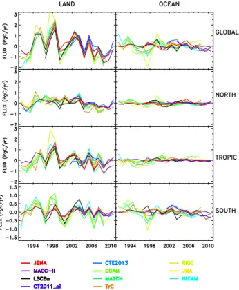
Figure 6 shows the interannual variability (IAV) for the northern, tropical and southern aggregated land and ocean regions. We refer to these as interannual carbon exchange anomalies (see Sect. 3.3).
All submissions tend to exhibit greater IAV on land ver-sus ocean, particularly in the tropical latitude band. For the 1996–2007 period, the mean across all inversions of the standard deviation of the annual means over land is around 1.06 Pg C yr−1versus 0.34 Pg C yr−1over the ocean. Over land, we obtain 0.67 Pg C yr−1for the tropics and only around 0.38 g C m−2yr−1 for both northern and southern land. This is consistent with i) numerous inversion stud-ies over the past two decades (e.g. Bousquet et al., 2000; Baker et al., 2006) and (ii) several analyses of land ecosystem model results (i.e., Sitch et al., 2008) and ocean model results (i.e., Le Quéré et al., 2000, 2010). Note also that it may re-flect in part the tighter prior constraint most inversions apply to ocean regions relative to the land. Within the land aggre-gates, the tropical land exhibits the greatest amount of inter-annual variability while for the oceans, greater interinter-annual variability is seen in the Southern Ocean (mainly associated with the 1997/1998 time period).
It is worth noting that only the two CT inversion submis-sions include interannual variability in their prior fluxes (see Fig. S3 in Supplement). The CT2011_oi/CTE2013 prior flux may be influencing their tropical land estimates in 2006 when this submission shows a carbon exchange anomaly in the tropical land that is more positive than the other submitted results.
The phasing of the carbon exchange anomalies shows con-sistency among the inversion submissions. For the global total, the peak positive anomaly associated with the large 1997/1998 El Niño event shows RIGC reaching their max-ima nearly one year sooner than the other submissions; in the tropics, NICAM also shows a broader peak for this event. This is likely due to the CO2emission signal from forest fires
in Indonesia in 1997 and northern Southeast Asia in 1998 as captured by the upper air measurements between Tokyo and Sydney (see Patra et al., 2005b for sensitivity results and detailed discussions). While some other inversions in-clude these upper air measurements, the choice of inverse set-up (particularly observation and prior errors) may limit the extent to which the data are fitted and consequently the
Fig. 5. Same as Fig. 4 but the breakdown of the Northern Hemisphere fluxes into (a) North America, (b) Europe, (c) North Asia, (d) N.
At-lantic, and (e) N. Pacific. Numbers in parenthesis represent the mean flux and the standard deviation across all inversions.
Fig. 6. Annual mean anomalies of the individual participating
in-version posterior flux estimates. Shown here are the fossil-fuel-corrected natural land (first column) and natural ocean (second col-umn) carbon exchange for the same regions as Fig. 4: global, north (> 25◦N), tropics (25◦S–25◦N) and south (< 25◦S).
magnitude of any emissions estimate from Indonesian fires. Most inversions place the primary driver of the 1997/1998 positive anomaly in the tropical land region though RIGC, CCAM and MATCH also place a positive anomaly in the southern land partly offset by a negative anomaly in the Southern Ocean region. Note that such a negative South-ern Ocean anomaly in 1997 is above 1 Pg C yr−1 in RIGC
and that it compensates for the large positive tropical land anomaly during the same year.
Overall, the RIGC inversion shows the greatest amount of IAV on land and ocean compared to the remaining inver-sions. For the 1996–2007 period, the standard deviation of the annual means over land is 1.60 Pg C yr−1for RIGC, only 0.93 Pg C yr−1for JMA, and between 1.0 and 1.25 Pg C yr−1 for JENA/MACC-II/CCAM/MATCH/TrC/NICAM inver-sions. For the shorter 2001–2008 period, both CT in-versions show the smallest IAV on land with a stan-dard deviation nearly half that of the remaining inversions (∼ 0.5–0.7 Pg C yr−1versus ∼ 1.0 Pg C yr−1). Differences in the amount of IAV arise primarily from differences in prior flux uncertainties as well as in observation errors. For in-stance, RIGC uses prior uncertainties over ocean regions that are similar to those over land regions (see Table 2), while most other systems have much larger uncertainties over land than over ocean regions. Such a difference probably explains the largest IAV in RIGC. Futher evaluation of the simulated atmospheric concentrations against independent data (i.e. not assimilated) may help to validate the estimated flux IAV from each inversion.
Positive global land anomalies across the submissions oc-cur for the following years: 1995, 1997/1998, 2002/2003, 2005/2006, and 2007/2008. All of these positive anomalies
appear to be driven by the tropical land region though the 2002/2003 anomaly shows potential contributions from the northern and southern land as well.
Ocean interannual variability shows less consistency among the inversions. In the Southern Ocean, all inver-sions except the LSCEa inversion show uptake during the 1997/1998 time period (JENA shows little anomalous flux over this time period). Inversions with larger ocean uptake often have larger southern land sources through this pe-riod, suggesting compensating errors. For instance, RIGC, CCAM and MATCH present a significant anti-correlation be-tween the annual southern-land- and Southern-Ocean-fluxes, around −0.6. Overall the spread across the ocean flux esti-mates tends to decrease through time. It would be valuable if future work could explore whether this reduction in spread is related to improved atmospheric CO2networks over time.
4.4 Long-term trends
Long-term trends are difficult to determine from this set of inversions for a number of reasons. First, the length of the inversions considered here is at most 21 yr, with some inver-sions less than half this length. Second, as noted above, in-terannual variations are large, making long-term trends unre-liable. In particular, ENSO events such as that of 1997–1998 cause variations with somewhat irregular frequency and magnitude, while the eruption of Mt Pinatubo in 1991 likely influences the early years of those inversions that covered longer time periods. Finally the choice and implementation of the fossil fuel CO2emission prior could lead to apparent
trends, particularly at regional scales.
With these caveats in mind, Fig. 7 displays the long-term annual anomalies obtained from smoothing the IAV signal in time (see Sect. 3.3). Most inversions show a tendency to-wards increasing land carbon uptake in the global and north-ern land domains from the late 1990s up to 2008 and then a tendency towards decreasing land uptake. Linear fits to the annual land totals for each inversion give on average an in-crease of 0.12 Pg C yr−1 over the 1995–2008 period (stan-dard deviation of 0.05 Pg C yr−1) explained mainly by the northern land. The tropical land response is less clear with the 1990s potentially dominated by Pinatubo-related nega-tive anomalies early in the decade and ENSO-related posi-tive anomalies later in the decade. In the 2000s, the tropi-cal land trend exhibits a large spread across the participating inversions, with four inversions showing an increased sink (JENA, MACC-II, RIGC, NICAM). The southern land flux estimates appear to be dominated by periodic behavior rather than a trend. The estimated ocean fluxes are approximately constant in time. However, a relatively small increase of the global ocean uptake in the 2000s is visible in a few inver-sions (both CT, and to a small extent JMA). Note that in the case of the two CT systems, such a trend was also present in their a priori flux estimates (see Supplement, Fig. S5). Un-like recent ocean flux synthesis combining ocean models and
Fig. 7. Smoothed annual mean anomalies (smoothing window of
3 yr) carbon exchange from the individual participating inversions. Shown here are the natural land “fossil-fuel-corrected” (first col-umn) and natural ocean (second colcol-umn) carbon exchange aggre-gated over the Globe, north (> 25◦N), tropics (25◦S–25◦N) and south (< 25◦S).
ocean interior data (i.e., Sarmiento et al., 2010; Wanninkhof et al., 2013) the atmospheric inversions still probably lack the atmospheric observational constraint to unambiguously identify large-scale ocean flux trends.
Figure 8 divides the northern land into regions, show-ing the three-year smoothed fluxes for North America, Eu-rope and North Asia (see region boundaries in Supplement, Fig. S7). The figure shows a tendency towards increasing land uptake for North Asia from the mid-1990s to 2008 (around 0.7 Pg C), while the European and North American uptake remain more constant. The trend over North Asia tends to reverse after 2008 with a decreasing carbon uptake in JENA, MACC-II and both CT inversions. However, these are all regions with significant fossil fuel CO2emissions and it is
important to understand how these trends could be influenced by how each inversion includes fossil fuel emissions and how the results may be influenced by the fossil fuel correction ap-plied to the results. For example, some inversions use global fossil fuel emissions that increase in time but with a spatial distribution that does not vary over time. Thus the emissions for each region are forced to increase at the same rate. If this did not occur in reality, then any deviation from that global rate would become an artificial trend in the “natural” flux
Fig. 8. Same as Fig. 7 but with a breakdown of the northern land
fluxes into (a) North America, (b) Europe, and (c) North Asia.
estimated for that region. Note that without the “fossil fuel correction” the smoothed fluxes for North Asia have a larger spread and do not exhibit an increasing carbon uptake from the mid 1990s to 2008 (not shown).
4.5 Mean seasonal cycle
Figures 9 and 10 show the mean seasonal cycle (defined in Sect. 3.3) on land and ocean for the latitudinal aggregate re-gions and for three continental rere-gions. Note that the land and ocean panels use different vertical scales. For this diagnostic, we consider the raw natural fluxes and not the “fossil-fuel-corrected” fluxes, to avoid any spurious monthly flux correc-tions, given that some inversions use monthly variations in fossil fuel emission. The global land seasonality is driven by the northern land with close agreement regarding both the magnitude and phasing of the growing season and dormant season fluxes. We next discuss, in more detail, the results for each region and for the continental breakdown of the north-ern land aggregate.
For northern land, the amplitude of the seasonal cycle is close to 3.2 Pg C month−1 (RIGC having the smallest
Fig. 9. Mean seasonal cycle of the posterior carbon exchange for the
individual participating inversion submissions. Shown here are the natural land (first column) and natural ocean (second column) car-bon exchange aggregated over the Northern Hemisphere (> 25◦N), the tropics (25◦S–25◦N) and the Southern Hemisphere (< 25◦S).
amplitude with 3.0 Pg C month−1 and TrC the largest with 3.5 Pg C month−1) and the peak of the growing season is lo-cated in July for all inversions. The growing season shows a larger spread across the inversions than the dormant sea-son with the LSCEa, MACC-II and JENA systems having a slightly earlier onset of the growing season carbon drawdown than the other systems. The peak carbon uptake is greatest for the TrC and NICAM inversions with the NICAM inver-sion compensating somewhat through slightly greater dor-mant season fluxes. Ocean flux seasonal cycles show less agreement in both phase and magnitude across the inver-sions. The prior ocean fluxes for this region tend to show carbon release in the July–September period (Supplement, Fig. S6); this seasonality is maintained by some of the in-versions, while others (e.g. JENA, TrC, RIGC) show a small uptake during summer. Since the amplitude of the northern ocean seasonality is much smaller than that of the land, a small error in the allocation of seasonality between land and ocean regions can more easily change the phase of the esti-mated ocean seasonality between inversions than that of the land seasonality.
Seasonality for the tropical land is smaller than the north-ern land, with most inversions giving maximum uptake around August to October. The LSCEa and MACC-II inver-sions give larger amplitude seasonality with maximum up-take earlier in the year, from June–August. The constraint from the prior ORCHIDEE land surface model used by the LSCEa/MACC-II inversions is the likely source of this difference (Supplement Fig. S6), given the similarities be-tween the prior and posterior fluxes that we obtain for most
Fig. 10. Same as Fig. 9 but the breakdown of the land
North-ern Hemisphere fluxes into (a) North America, (b) Europe, and
(c) North Asia.
inversions. The seasonality of the tropical oceans shows much smaller amplitude than the tropical land and with less agreement in phase and magnitude. NICAM and RIGC in-versions show larger emission peaks than other inin-versions, in May/June and October/November, respectively, a feature probably linked to larger prior ocean flux uncertainties for RIGC (0.8 Pg C yr−1, see Table 2).
Seasonality in the southern land shows reasonable consis-tency across the inversions in terms of phasing. Maximum carbon uptake across the inversions spans the February to April time period. The peak of the dormant season carbon emission varies from June to October depending upon the in-version. Both CT variants show the earliest peak in dormant season fluxes (roughly June) while MATCH, RIGC, CCAM, JENA and JMA show peak fluxes in October. LSCEa has two emission peaks in June and September. Southern Ocean fluxes show general agreement with uptake in the austral winter/spring, opposing the seasonality of the southern land. The amplitude of the estimated ocean seasonality is larger than in the prior flux, but with similar phasing. The RIGC
in-version gives large monthly variations from February to June, not seen in any other system.
Figure 10 shows the seasonality of estimated fluxes for North America, Europe and North Asia. There is broad agreement between the inversions for each region, all show-ing characteristically different patterns of seasonality be-tween regions. Uptake begins earlier for Europe than for the other regions, while North Asia shows the largest seasonal-ity, because this is the largest land area of the three regions. These differences are also seen in the prior fluxes (Supple-ment, Fig. S6) used by most inversions, which are mainly based on the CASA model (Randerson et al., 1997). It is worth noting that the inversions that do not use this prior (MACC-II, LSCEa, JENA) nevertheless largely agree with the other inversion estimates. Given the significant differ-ences between the MACC-II/LSCEa prior (both based on two versions of the same land model) and the other priors (Supplement, Fig. S6), the similarity of the posterior fluxes indicates that the seasonality is driven primarily by the atmo-spheric data rather than the prior flux. A weak influence from the prior may be the reason why both LSCEa and MACC-II inversions show earlier maximum uptake in the North Amer-ican and European regions.
For Europe there seems to be greater inversion spread for the early part of the growing season than for the onset of senescence. For North Asia, some inversions show increased sources in April–May and September–November. The peak uptake in July–August is more variable across inversions for this region than for the other northern land regions. This is most likely because this region is large (encompassing the Middle East, India, parts of China and Siberia) and is not as well sampled by atmospheric measurements as Europe and North America. Note also that the JENA inversion with no prior land flux seasonality tends to produce an earlier start of the growing season net flux, than the other inversions.
The integrals of the growing season net flux (GSNF, i.e., the period when the net flux is negative) and the dormant season net flux (DSNF, i.e., the period when the net flux is positive) vary significantly between the inversions. For the GSNF/DSNF, the mean and stan-dard deviation across the inversions, calculated for the 2001–2004 period, are: −2.12 × 0.21/1.45 × 0.36 Pg C for North America, −1.47 × 0.21/1.08 × 0.27 Pg C for Europe, and −2.68 × 0.31/1.66 × 0.29 Pg C for North Asia. The DSNF appears to be slightly more variable across the inver-sions than the GSNF.
5 Interpretation of regional fluxes and uncertainty estimates
Analysis of the estimated inversion natural fluxes has shown that differences occur at the global scale through different representations of fossil fuel emissions, and that differences between inversions generally increase as the region being




![[PDF] Cours Pascal les structures itératives pdf | formation informatique](data:image/gif;base64,R0lGODlhAQABAIAAAP///wAAACH5BAEAAAAALAAAAAABAAEAAAICRAEAOw==)