HAL Id: hal-01092615
https://hal.archives-ouvertes.fr/hal-01092615v3
Submitted on 26 May 2015
HAL is a multi-disciplinary open access
archive for the deposit and dissemination of
sci-entific research documents, whether they are
pub-lished or not. The documents may come from
teaching and research institutions in France or
abroad, or from public or private research centers.
L’archive ouverte pluridisciplinaire HAL, est
destinée au dépôt et à la diffusion de documents
scientifiques de niveau recherche, publiés ou non,
émanant des établissements d’enseignement et de
recherche français ou étrangers, des laboratoires
publics ou privés.
mobility
Maxime Lenormand, Thomas Louail, Oliva García Cantú, Miguel Picornell,
Ricardo Herranz, Juan Murillo Arias, Marc Barthelemy, Maxi San Miguel,
José Javier Ramasco
To cite this version:
Maxime Lenormand, Thomas Louail, Oliva García Cantú, Miguel Picornell, Ricardo Herranz, et
al.. Influence of sociodemographic characteristics on human mobility. Scientific Reports, Nature
Publishing Group, 2015, 5 (10075), pp.10075. �10.1038/srep10075�. �hal-01092615v3�
Maxime Lenormand,1 Thomas Louail,2, 3 Oliva G. Cant´u-Ros,4 Miguel Picornell,4 Ricardo
Herranz,4 Juan Murillo Arias,5 Marc Barthelemy,2, 6 Maxi San Miguel,1 and Jos´e J. Ramasco1
1Instituto de F´ısica Interdisciplinar y Sistemas Complejos IFISC (CSIC-UIB),
Campus UIB, 07122 Palma de Mallorca, Spain
2
Institut de Physique Th´eorique, CEA-CNRS (URA 2306), F-91191, Gif-sur-Yvette, France
3G´eographie-Cit´es, CNRS-Paris 1-Paris 7 (UMR 8504), 13 rue du four, FR-75006 Paris, France
4Nommon Solutions and Technologies, calle Ca˜nas 8, 28043 Madrid, Spain
5
BBVA Data & Analytics, Avenida de Burgos 16D, 28036 Madrid, Spain
6
Centre d’Analyse et de Math´ematique Sociales, EHESS-CNRS (UMR 8557),
190-198 avenue de France, FR-75013 Paris, France
Human mobility has been traditionally studied using surveys that deliver snapshots of population displacement patterns. The growing accessibility to ICT information from portable digital media has recently opened the possibility of exploring human behavior at high spatio-temporal resolutions. Mobile phone records, geolocated tweets, check-ins from Foursquare or geotagged photos, have contributed to this purpose at different scales, from cities to countries, in different world areas. Many previous works lacked, however, details on the individuals’ attributes such as age or gender. In this work, we analyze credit-card records from Barcelona and Madrid and by examining the geolocated credit-card transactions of individuals living in the two provinces, we find that the mobility patterns vary according to gender, age and occupation. Differences in distance traveled and travel purpose are observed between younger and older people, but, curiously, either between males and females of similar age. While mobility displays some generic features, here we show that sociodemographic characteristics play a relevant role and must be taken into account for mobility and epidemiological modelization.
I. INTRODUCTION
Everyday, billions of individuals generate a large volume of geolocated data by using their mobile phone, GPS, public transport cards or credit cards. Such a vast amount of data is bringing new
opportu-nities for the research in socio-technical systems [1–
3]. Indeed, geolocated data allow the identification of
when and where people interact with or through ICT tools. Each time someone makes a phone call or pays with a credit card the event gets registered contribut-ing to massive databases with potential to provide
use-ful insights on human behavior and mobility [4–9]. For
example, the authors of Refs. [6, 7] used credit card
and mobile phone datasets to study statistical char-acteristics of mobility patterns and showed that the distribution of displacement of all users can be ap-proximated by a Levy law. Recently, geolocated data has been also employed to study the spatial structure
of cities by detecting hotspots [10] or to characterize
land use patterns in urban areas [11–15] with mobile
phone records, Twitter data [16] or both together [17].
On a larger scale, comparisons and relations between
different cities [18] or even between countries [19,20]
have also been also investigated.
Beyond mere location, some datasets offer the op-portunity to gather extra information about the type and duration of the interaction or the operation
through ICT tools. For instance, it is possible to
know from mobile phone records where and when an individual makes a call, but sometimes information such as the ID of the callee and the call duration are also available. This information enables researchers to move further on the study of human behavior by analyzing the structure, intensity and spatial
proper-ties of social interactions. Some examples include the
analysis of the structure of social networks [21–27],
the correlation between mobility and social network
[28–30], information diffusion [31] and the role played
by social groups [26,32].
However, many previous studies lack sociodemo-graphic resolution on the characteristics of the indi-viduals. Except for some features such as language or
place of work and/or residence identified in [19, 33],
information about gender, age or occupation are typ-ically missing from studies based on ICT data. This information is of great relevance to characerize the city structure, to estimate population needs in ur-ban planning, transport demand and also for public health. For example, regarding age, knowing the ar-eas of concentration of younger and older population helps to optimize infrastructure such as location of schools, care facilities, etc. Another aspect for which this information is relevant is the modeling of infec-tious diseases spreading. The models rely on the in-terplay among hosts, which is related to their location and mobility. Recent epidemic modeling has incorpo-rated mobility information as a way to get closer to
real disease spreading [4,34–47]. Additionally,
demo-graphic factors such as age or gender can also play an important role in disease transmission and, therefore, must be taken into account when modeling certain
infections [48,50–54]. Furthermore, in a sort of
feed-back loop, these sociodemographic factors influence mobility as well.
Some works based on smaller-scale surveys point out towards a number of significant differences be-tween men and women in terms of their travel
pur-poses and the activities they pursue [55–57]. More
recently, quantitative studies of social networks
Figure 1: Maps of the transactions. The red dots represent the locations of the transactions on a map of the province of Madrid (a) and Barcelona (b). The small areas correspond to postcodes.
namics have also shown that people behave differently
according to the gender and age [58,59]. In this paper,
we go beyond by analyzing a credit card use database containing over 40 million card transactions in or-der to explore consumption and mobility patterns of bank customers in the two most populated provinces of Spain according to three sociodemographic charac-teristics: gender, age and occupation.
II. MATERIALS AND METHODS
A. Dataset description
Our dataset comes from an extraction of the Banco Bilbao Vizcaya Argentaria (BBVA) database on credit card transactions. Different extractions of this data
have been used in open data challenges [60] and other
scientific works [61]. The data contains
informa-tion about 40 million bank card transacinforma-tions made in the provinces of Madrid and Barcelona in 2011. Each transaction is characterized by its amount (in euro currency) and the time when the transaction
has occurred. Each transaction is also linked to a
customer and a business using anonymized customer and business IDs. Customers are identified with an anonymized customer ID connected with sociodemo-graphic characteristics (gender, age and occupation) and the postcode of his/her place of residence. For convenience sake, we consider five age groups (]15, 30], ]30, 45], ]45, 60], ]60, 75], > 75) and five types of occu-pations (student, unemployed, employed, homemaker, and retired). In the same way, businesses are identi-fied with an anonymized business ID, a business cate-gory (accommodation, automotive industry, bars and restaurants, etc.) and the geographical coordinates of the credit card terminal.
The geographical extent of our data is restricted to the provinces of Barcelona and Madrid. For both
case studies, we only consider the credit card pay-ments made in the province by individuals living in
the province (Figure1). TableI presents some basic
statistics on the data collected. Both provinces have similar features in terms of population size, area and number of businesses, but the number of users and transactions are higher in Madrid than in Barcelona. The number of users represents about 8% of the to-tal census population in Madrid and 5% of that of Barcelona.
TABLE I: Summary statistics of the two provinces
Statistics Barcelona Madrid
Number of postcodes 368 271 Number of inhabitants 5,540,925 6,489,680 Area (km2) 7,733 8,022 Number of customers 270,205 531,818 Number of transactions 13,077,178 24,920,896 Number of businesses 111,956 109,707 III. RESULTS
The statistical features of the data for Barcelona
and Madrid are very similar. Therefore, the data
is aggregated for analyzing general properties in the next two sections and segregated later in the third one to study mobility patterns. The aggregation pro-vides higher statistical power, while the disaggrega-tion is needed due to the different geographical shapes of both provinces. Due to the optimization of space, only figures obtained for Madrid are displayed in the third section on mobility. Still equivalent results for Barcelona are found and can be seen in appendix
(Fig-0.0 0.2 0.4 0.6 0.8 BBVA Census Gender Propor tion of customers BBVA Census Age Occupation n 0 10 20 30 40 Number of T ransactions 0 500 1000 1500 2000 Amount of Mone y Man W oman 0 20 40 60 80 Amount per T ransaction ]15,30] ]30,45] ]45,60] ]60,75] >75 Student Unemplo y ed Emplo y ed Homemak er Retired
Figure 2: Descriptive statistics according to the individual sociodemographic characteristics. From top to bottom, proportion of individuals, median number of transactions per user and per year, median amount of money spent per user and per year (in euro) and median of the average amount of money spent per transaction (in euro) according to, from left to right, the gender, the age and the occupation.
ures S9 - S15).
A. General features
In order to have a first look at the data, we plot in
Figure2 some descriptive statistics about individuals
according to their sociodemographic characteristics.
Figure 2 shows the proportion of individuals
accord-ing to gender, age and occupation in the dataset and the corresponding fractions as observed in the
cen-sus [62]. We note an over-representation of men and
middle-aged individuals (30-60) in the dataset
com-pared to census data. Moreover, employed people
represent about 80% of the individuals, which is two times higher than the proportion of employed people in Spain. Therefore, since the data are not represen-tative of the population, in the rest of the manuscript only indicators and measures normalized by the total number of individuals in each groups will be consid-ered. It is also important to note that the three
distri-butions are not independent, for example, the propor-tion of individuals according to the age is not the same for student and retired individuals. In the same way, the proportion of individuals according to the occu-pation is different for men and women. For example, there are more female homemakers than male home-makers. For more details, histograms of the three joint distributions are available in appendix (Figure S1, S2, and S3).
To highlight differences between individuals hav-ing different sociodemographic characteristics, we also
plot on Figure 2 the median number of transactions
per user, the median amount of money spent per user and the median average amount of money spent per transaction per user. We used the median instead of the average because the distributions exhibits a large number of outliers (see Figure S4, S5 and S6 in ap-pendix for more details). It can be observed that in-dividuals do not spend their money in the same way according to whether they are men or women, young or old and active or inactive. For instance, the
num-0.00 0.05 0.10 0.15 0.20 0.25 0.30 0.35 Man Woman 0.00 0.05 0.10 0.15 0.20 0.25 0.30
Propor
tion of mone
y spent
]15,30] ]30,45] ]45,60] ]60,75] >75 Accomodation A utomotiv e industr y Bar / Restaur ant Book / CD / Stationer y F ashion F ood / Hyper mar k ets Health Home Leisure Spor ts / T o ys T echnology Transpor t T ra v el Agencies W ellness / Beauty Other 0.0 0.1 0.2 0.3 0.4 Student Unemployed Employed Homemaker RetiredFigure 3: Average fraction of money spent by an individual according to the business category and his/her sociodemographic characteristics. From the top to the bottom: gender, age and occupation.
ber of transactions and the amount of money spent is higher for women than for men and decreases with age. Furthermore, they are also higher for employed persons and homemakers than for unemployed indi-viduals, students and retired people (which is proba-bly related to the age). Inversely, the average amount of money spent per transaction is higher for men than women and increases with age.
To investigate the influence of sociodemographics on the way people spend their money, we plot on
Figure 3 the average fraction of money spent by an
individual according to the business category and his/her sociodemographic characteristics. Since the total amount of money spent in 2011 is different from one individual to another, the distribution has been normalized for each user by the total amount of money
he/she spent during the year. Note that the
dis-tribution is very different for men and women. In-deed, women spend more money than men in Fashion, Food/Hypermarkets, Health and Wellness/Beauty whereas men spend more money than women in Au-tomotive Industry, Bar/Restaurants, Technology and
Transport. We also find that the proportion of money spent in Fashion, Food/Hypermarkets, Sports/Toys, Technology and Transport globally decreases with
age. Inversely, the amount of money spent in
Au-tomotive Industry, Health, Travel Agencies and Well-ness/Beauty increases with age. Finally, the differ-ences between people having different occupation are explored. For instance, students spend more money in Bar/Restaurant, Fashion, Sports/Toys and Tech-nology than others types of occupation.
Since the proportion of individuals according to the occupation is different for men and women, and in or-der to take away potential bias, we have studied the average fraction of money spent by an individual ac-cording to the business category and his/her sociode-mographic characteristics but only for employed in-dividuals. We reach the same conclusions as for the overall sample, see Figure S7 in appendix.
0.00 0.02 0.04 0.06 0.08 0.10
(a)
Time of day (h)
Propor tion of mone y spent 6 12 18 0 6 12 18 0 6 12 18 0 6 12 18 Total Cluster 1 Cluster 2 Man W oman ]15,30] ]30,45] ]45,60] ]60,75] >75 Student Unemplo y ed Emplo y ed Homemak er Retired(b)
0.0 0.1 0.2 0.3 0.4 0.5 0.6 0.7 Propor tion of customersFigure 4: Time evolution of the amount of money spent. (a) Average amount spent per day as a function of the hour of the day in total and according to the cluster. From left to right: weekdays (aggregation from Monday to Thursday), Friday, Saturday and Sunday. (b) Proportion of individuals in total and in each cluster according to, from left to right, the gender, the age and the occupation.
B. Time evolution of the amount of money spent
To study how the amount of money spent by BBVA customers changes over time during an average week, the days of the week have been divided into four groups: one, from Monday to Thursday represent-ing a normal workrepresent-ing day (hereafter called W D) and three more for Friday, Saturday and Sunday (here-after called F ri, Sat and Sun). The average amount of money spent per day as a function of the hour of
the day is displayed in Figure4a (gray curve).
Glob-ally, the amount of money spent is significantly higher during the week days, Friday and Saturday than on Sunday. This can be explained by the fact that most of the business were closed on Sunday in Spain in the time that the data was collected. The activity on Sun-day takes place between 10am and 7pm with a small peak around 4pm. During the week days, Friday and Saturday money is spent between 8am and 10pm. For these days the curves show two peaks, one around noon and another one around 7pm. It is interesting to note that for the week days and Friday the second peak is higher than the first one whereas the oppo-site behavior is observed on Saturday. A small peak around 11pm corresponding to the nightlife activity is
also observed for the three first days.
To go further in the analysis, a k-means
cluster-ing algorithm with Euclidean distance [63] is applied
in order to identify clusters naturally present in the data. The purpose is to cluster together individuals exhibiting temporal distribution of money spent. The total amount of money spent in 2011 is different from one individual to another so we have normalized the temporal distribution of money spent for each user by the total amount of money he/she spent in 2011. To choose the number of clusters, we use the pseudo-F statistics which describes the ratio of between-cluster
variance to within cluster variance [64]. The optimal
number of clusters is the one for which the highest pseudo-F value is obtained, in our case we found two opposite clusters (see Figure S8 in appendix for more
details). Figure4a displays the results of the
cluster-ing analysis, we observe an opposition between active and inactive individuals. The first cluster represents one third of the individuals and is characterized by a higher activity during the morning and during week-days in opposition with the second cluster in which individuals tend to spend more money after 6pm and during week end days. It is interesting to note that the first cluster is over-represented by women, old people
Total ∆tRhouri P
(
∆t)
100 101 102 103 104 10- 9 10- 8 10- 7 10- 6 10- 5 10- 4 10- 3 10- 2 10- 1 100(a)
Man Woman ∆tRhouri P(
∆t)
100 101 102 103 104 10- 9 10- 8 10- 7 10- 6 10- 5 10- 4 10- 3 10- 2 10- 1 100(b)
]15,30] ]30,45] ]45,60] ]60,75] >75 ∆tRhouri P(
∆t)
100 101 102 103 104 10- 9 10- 8 10- 7 10- 6 10- 5 10- 4 10- 3 10- 2 10- 1 100(c)
Student Unemployed Employed Homemaker Retired ∆tRhouri P(
∆t)
100 101 102 103 104 10- 9 10- 8 10- 7 10- 6 10- 5 10- 4 10- 3 10- 2 10- 1 100(d)
0 50 100 150 200 250 300 350 ∆t Rho ursi 0 100 200 300 400 500 600 ∆t Rho ursi 0 100 200 300 400 500 ∆t Rho ursiFigure 5: Inter-event time distribution P (∆t). (a) Probability density function of ∆t. (b) - (d) Probability density
function of ∆t according to the gender (b), the age (c) and the occupation (d). The insets show the Tukey boxplot of
the distributions, the black points represent the average.
and homemaker and retired individuals compared to
the whole population (Figure4b).
C. Mobility patterns
In order to characterize mobility patterns of each
user, we have considered three variables: ∆t, the time
elapsed between two consecutive transactions, ∆r, the
distance traveled between two consecutive
transac-tions, and rg, the radius of gyration [7]. The radius
of gyration is defined as rg= v u u t 1 n n X k=1 ( ~pk− ~pc)2, (1)
where ~pk represents the kth position of the user
dis-placements in 2011 and ~pc= n1Pnk=1p~k is the center
of mass of his/her motions. It is important to note
that rg is defined per user whereas ∆t and ∆r are
computed for each displacement. Although ∆rand rg
are related, ∆rinforms us on the distance traveled by
users, which might depend on the frequency at which
each person uses its credit card, whereas rg gives us a
more holistic view of how people moves around their
centers of mass. To avoid the introduction of bias
in the mobility patterns analysis, all the consecutive user’s positions geo-located in the province and the distances between them are considered whatever the elapsed time between consecutive transactions.
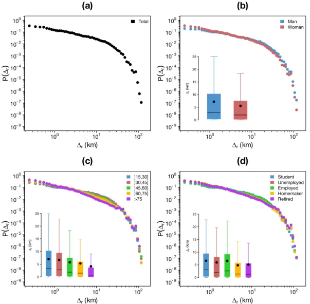
Figures 5a, 6a and 7a display the probability
den-sity function of the three variables. The distribution
of ∆t is a decreasing density function exhibiting
cir-cadian rhythms. The average and median time be-tween two transaction are, respectively, around 5 days
and 2 days. The distribution of ∆r show two
dif-ferent regimes. First the distribution exhibits a slow decay, and then, beyond 40 kilometers the distribu-tion is characterized by a rapid decay. This cutoff
Total ∆r(km) P
(
∆r)
100 101 102 10- 9 10- 8 10- 7 10- 6 10- 5 10- 4 10- 3 10- 2 10- 1 100(a)
Man Woman ∆r(km) P(
∆r)
100 101 102 10- 9 10- 8 10- 7 10- 6 10- 5 10- 4 10- 3 10- 2 10- 1 100(b)
]15,30] ]30,45] ]45,60] ]60,75] >75 ∆r(km) P(
∆r)
100 101 102 10- 9 10- 8 10- 7 10- 6 10- 5 10- 4 10- 3 10- 2 10- 1 100(c)
Student Unemployed Employed Homemaker Retired ∆r(km) P(
∆r)
100 101 102 10- 9 10- 8 10- 7 10- 6 10- 5 10- 4 10- 3 10- 2 10- 1 100(d)
0 5 10 15 20 25 ∆r (k m ) 0 5 10 15 20 25 ∆r (k m ) 0 5 10 15 20 25 ∆r (k m )Figure 6: Distribution of the distance traveled by an individual between two consecutive transactions
P (∆r). (a) Probability density function of ∆r. (b) - (d) Probability density function of ∆r according to the gender (b),
the age (c) and the occupation (d). The insets show the Tukey boxplot of the distributions, the black points represent the average.
is introduced by the limited geographical scale of the
provinces. The probability density function P (rg)
in-creases very slowly until reaching a maximum around 6 kilometers and then the distribution is characterized by a rapid decay.
In this work we have also assessed the influence of sociodemographic characteristics on the individual mobility patterns. The results obtained are plotted
on the Figure5,6 and7. For each sociodemographic
characteristic and each variable, we performed two non-parametric tests to assess the statistical signifi-cance of the differences between the different type of
users’ mobility using the MannWhitney U test [65] to
compare the distributions and the Mood’s median test
[66] to compare the medians. For both case studies the
differences between distributions and medians are
al-ways significant (p-values lower than 10−4) except for
the difference between radius of gyration of individ-uals of age between 15 and 30 and those between 30
and 45 in Barcelona.
Figure 5 displays the inter-event time distribution
according to the gender (Figure 5b), the age
(Fig-ure 5c) and the occupation (Figure 5d). The
aver-age and median inter-event time are higher for men than women and increases with age. They are also higher for unemployed individuals, students and re-tired people than for employed persons and home-makers. We observe an negative correlation between the time elapsed between two consecutive transac-tions and the number of transactransac-tions per individual described in the first section.
The results obtained for ∆r and rg are plotted
in Figure 6 and 7, respectively. Based on these
re-sults, one can understand that, depending on his/her sociodemographic characteristics, an individual can travel short or long distances and stays more or less close to his/her center of mass. Three main differences are observed. First, women travel shorter distances
rg(km) P
(
rg)
100 101 102 10- 6 10- 5 10- 4 10- 3 10- 2 10- 1 100(a)
Man Woman rg(km) P(
rg)
100 101 102 10- 6 10- 5 10- 4 10- 3 10- 2 10- 1 100(b)
]15,30] ]30,45] ]45,60] ]60,75] >75 rg(km) P(
rg)
100 101 102 10- 6 10- 5 10- 4 10- 3 10- 2 10- 1 100(c)
Student Unemployed Employed Homemaker Retired rg(km) P(
rg)
100 101 102 10- 6 10- 5 10- 4 10- 3 10- 2 10- 1 100(d)
0 5 10 15 20 Rg (k m ) 0 5 10 15 20 Rg (k m ) 0 5 10 15 20 Rg (k m )Figure 7: Distribution of the radius of gyration P (rg). (a) Probability density function of rg. (b) - (d) Probability
density function of rgaccording to the gender (b), the age (c) and the occupation (d). The insets show the Tukey boxplot
of the distributions, the black points represent the average.
2 4 6 8 (a) Man Woman 1 > ]1,3] ]3,6] ]6,12] ]12,18] ]18,24] ]24,30] ]30,36] ]36,42] ]42,48] ]48,60] ]60,72] ]72,96] ]96,120] > 120 ∆t (hour) < ∆r > (km) 2 4 6 8 (b) ]15,30] ]30,45] ]45,60] ]60,75] >75 1 > ]1,3] ]3,6] ]6,12] ]12,18] ]18,24] ]24,30] ]30,36] ]36,42] ]42,48] ]48,60] ]60,72] ]72,96] ]96,120] > 120 ∆t (hour) < ∆r > (km) 2 3 4 5 6 7 8 (c) Student Unemployed Employed Homemaker Retired 1 > ]1,3] ]3,6] ]6,12] ]12,18] ]18,24] ]24,30] ]30,36] ]36,42] ]42,48] ]48,60] ]60,72] ]72,96] ]96,120] > 120 ∆t (hour) < ∆r > (km)
Figure 8: Average < ∆r > value as a function of ∆t according to the gender (a), the age (b) and the
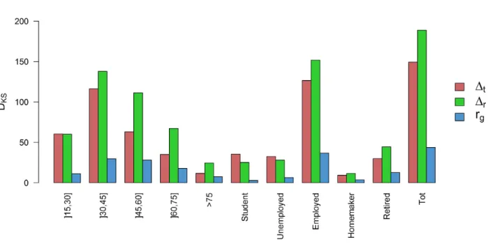
Figure 9: Kolmogorov-Smirnov distance between men and women’s ∆t distributions (in red), ∆r
dis-tributions (in green) and rg distributions (in blue) according to their sociodemographic characteristics.
than men and their trajectory stays closer to their center of mass. Second, the average distance trav-eled between two consecutive positions and the radius of gyration decrease with age. Finally, an opposition between active and inactive individual is highlighted. Indeed, retired, homemaker and, to a lesser extent, unemployed individuals travel shorter distances and stay closer to the center of mass than other people.
As previously mentioned, the distance traveled by an individual between two consecutive transactions might depend on the frequency at which an individ-ual uses his/her credit card, and therefore, the
differ-ences between people observed for ∆rcould be a
con-sequence of the differences observed for ∆t. Although
the same conclusion are reached for the radius of gyra-tion, which does not depend on the frequency at which someone uses his/her credit card, it could be
interest-ing to study how the average value of ∆revolves as a
function of ∆t according to the individual’s
sociode-mographic characteristics. We can observe in Figure
8 that the differences between the different types of
individuals in terms of distances traveled always ex-ist whatever the time elapsed between two
consecu-tive transactions. It is also worth noting that the
value of < ∆r > is not completely independent of
∆t. Obviously, for small values of ∆t (∆t < 6) the
value of < ∆r> increases with the value of ∆tdue to
physical constraints but we can also note a valley for
∆t∈ ]18, 30] followed by a peak for ∆t∈ ]30, 42]. This
phenomenon seems to be more pronounced for active people than for inactive people, possibly reflecting the home-to-work/school commuting.
Among all these comparisons, discrepancy in mobil-ity between men and women is the most challenging. In order to verify that this difference is significant and
it is not related to other sociodemographic variables, the Kolmogorov-Smirnov (KS) distance between men
and women’s ∆t, ∆r and rg distributions are
com-puted (Figure9). The Kolmogorov-Smirnov (KS)
dis-tance between two empirical probability distributions X and Y is defined as
DKS = sup
x
|FX(x) − FY(x)|, (2)
where FX and FY are the empirical cumulative
dis-tribution function of X and Y respectively. Since,
the sample size of both distributions may vary from one sociodemographic variable to another we need to
normalize DKS according to the sample sizes,
˜ DKS = r n XnY nX+ nY sup x |FX(x) − FY(x)|, (3)
where nX and nY represent the sample sizes of X
and Y , respectively. This allows for a direct
compar-isons of the Kolmogorov-Smirnov distances.
More-over, using this normalization, the null hypothesis that the two data samples come from the same
dis-tribution is rejected at level 0.001 if ˜DKS> 1.95.
First, we observe that a significant difference be-tween men and women appears whatever the sociode-mographic characteristic of the population is filtered
out (i.e. D˜KS is always higher than 1.95), which
means that on average, women have an inter-event time lower than men and men do longer journeys than women. Second, one can observe that this gendered difference is more important for middle age individual than for young and old people, but also that is more pronounced for employed people.
A
utomotiv
e industr
y
Bar / Restaur
ant
Book / CD / Stationer
y
F
ashion
F
ood / Hyper
mar
k
ets
Health
Home
Leisure
Spor
ts / T
o
ys
T
echnology
T
ranspor
t
T
ra
v
el Agencies
W
ellness / Beauty
T
otal
Total
Homemaker
Student
Retired
Unemployed
Employed
>75
]60,75]
]45,60]
]30,45]
]15,30]
Woman
Man
4 6 8 10 12 Distance (km)Figure 10: Average distance between individuals residence and business according to sociodemographics and business category. Distances are expressed in kilometer and are computed using the Haversine distance between the latitude and longitude coordinate of the centroid of the postcode of residence and the business’ latitude and longitude coordinates for each transaction.
To go further, we have studied too the influence of the individuals sociodemographic characteristics and the business category on the distance traveled be-tween home and business. To do so, we computed for each transaction the distance between the individual’s place of residence and the business. As residence loca-tion, we use the centroid of the individual’s postcode of residence. Finally, these distances were averaged according to individual and business type. These
av-erage distances can be observed in Figure10. First, we
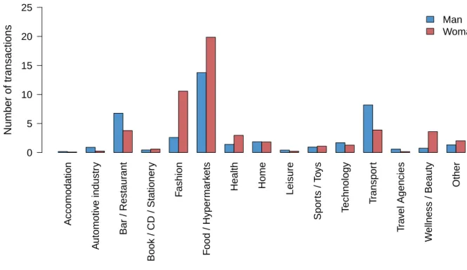
observe that the same differences between type of indi-viduals as the ones highlighted previously are obtained whatever the business category. For each business cat-egory, the distance between home and business is glob-ally higher for men than women, it decreases with age and it is higher for employed and student than for the other occupation categories. Although, the aver-age distance between home and business changes ac-cording to the category of business. Indeed, distances between home and businesses belonging to the cate-gories Food/Hypermarkets, Health, Wellness/Beauty and Book/CD/Stationery are lower than for the other categories. It is interesting to note that these business category are also the type of business in which the number of transactions is higher for women than for
men (Figure11). This partially explains why women
travel shorter distance than men to go shopping.
IV. DISCUSSION
In summary, we have shown in this study that it is possible to use information provided by credit card data to assess the influence of sociodemographic char-acteristics on the way people move and spend their
money. We highlighted differences in consumption
habits and mobility patterns of bank customers ac-cording to their gender, age and occupation. First, we shown that according to the business type the frac-tion of money spent can be very different from one individual to another. In particular, women tend to spend more money in Fashion, Food/Hypermarkets, Health and Wellness/Beauty than men whereas men spend more money than women in Automotive Indus-try, Bar/Restaurants, Technology and Transport. We have also studied the time evolution of the amount of money spent along the week according to the individ-ual’s sociodemographic characteristics. An opposition between two types of individuals has been identified. The temporal distribution of money spent by the first type of individuals which is over-represented by inac-tive people is characterized by a higher activity dur-ing the morndur-ing and durdur-ing weekdays in opposition with the second type of individuals more active after working hours and during week end days. Then, we investigated the properties of people mobility patterns using three variables: the time elapsed between two consecutive transactions, the distance traveled by an
Accomodation A utomotiv e industr y Bar / Restaur ant Book / CD / Stationer y F ashion F ood / Hyper mar k ets
Health Home Leisure
Spor ts / T o ys T echnology Transpor t T ra v el Agencies W ellness / Beauty Other 0 5 10 15 20 25 Man Woman Number of tr ansactions
Figure 11: Average number of transactions according to the gender and the business category.
individual between two consecutive transactions and
the radius of gyration. Three main differences
tween groups of people were identified: differences be-tween men and women, young and old people and ac-tive and inacac-tive individuals. In the three cases, peo-ple of the first group (men, young peopeo-ple and active people) travel shorter distances and their trajectory stays closer to their center of mass than individuals of the second groups (women, old individual and inactive people).
Among all the differences emphasized in this paper the one between men and women is the most difficult to explain. In all the comparisons we have carefully checked that this difference was not related to other sociodemographic variables and it was not the case. It could be interesting to verify whether this difference is related to other social characteristics such as the num-ber of children for example. Indeed, the fact that the difference in terms of mobility patterns between men and women is less pronounced for old people and stu-dents may reflect that women with children move dif-ferently than women without children. While further data is required to assess whether these differences
be-tween individuals are universal, i.e., to which extend they are specific or not to urban areas or the cities of the country analyzed, our results point toward the possibility that mobility may display significant dif-ferences for different types of individuals.
V. ACKNOWLEDGEMENTS
Partial financial support has been received from the Spanish Ministry of Economy (MINECO) and FEDER (EU) under projects MODASS (FIS2011-24785) and INTENSE@COSYP (FIS2012-30634), and from the EU Commission through projects EUNOIA, LASAGNE and INSIGHT. The work of ML has been funded under the PD/004/2013 project, from the Con-selleria de Educacin, Cultura y Universidades of the Government of the Balearic Islands and from the Eu-ropean Social Fund through the Balearic Islands ESF
operational program for 2013-2017. JJR
acknowl-edges funding from the Ram´on y Cajal program of
MINECO.
[1] Watts, D. J. A twenty-first century science. Nature 445, 489 (2007).
[2] Lazer, D. et al. Computational Social Science. Science 323, 721–723 (2009).
[3] Vespignani, A. Predicting the Behavior of Techno-Social Systems. Science 325, 425–428 (2009). [4] Chowell, G., Hyman, J., Eubank, S., Castillo-Chavez,
C. Scaling laws for the movement of people between
locations in a large city. Phys Rev E 68, 066102
(2003).
[5] Barrat, A., Barth´elemy, M., Pastor-Satorras, R.,
Vespignani, A. The architecture of complex weighted networks. Proc. Nat. Acad. Sci. USA 101, 3747–3752 (2004).
[6] Brockmann, D., Hufnagel, L. & Geisel, T. The scaling laws of human travel. Nature 439, 462–465 (2006). [7] Gonzalez, M. C., Hidalgo, C. A. & Barabasi, A.-L.
Understanding individual human mobility patterns. Nature 453, 779–782 (2008).
[8] Song, C., Qu, Z., Blumm, N. & Barab´asi, A.-L. Limits
of Predictability in Human Mobility. Science 327, 1018–1021 (2010).
[9] Bagrow, J. P. & Lin, Y.-R. Mesoscopic Structure and
Social Aspects of Human Mobility. PLoS ONE 7,
e37676 (2012).
[10] Louail, T. et al. From mobile phone data to the spatial structure of cities. Sci. Rep. 4, 5276 (2014).
[11] Ratti, C., Pulselli, R. M., Williams, S. & Frenchman, D. Mobile Landscapes: using location data from cell phones for urban analysis. Environment and Planning B: Planning and Design 33, 727–748 (2006). [12] Reades, J., Calabrese, F., Sevtsuk, A. & Ratti, C.
Cel-lular Census: Explorations in Urban Data Collection. Pervasive Computing, IEEE 6, 30–38 (2007). [13] Soto, V. & Fr´ıas-Mart´ınez, E. Automated land use
identification using cell-phone records. In Proceedings of the 3rd ACM international workshop on MobiArch, HotPlanet ’11, 17–22 (ACM, New York, NY, USA, 2011).
[14] Pei, T., Sobolevsky, S., Ratti, C., Shaw, S. L. & Zhou, C. A new insight into land use classification
based on aggregated mobile phone data. ArXiv
e-print arxiv:1310.6129 (2013).
[15] Toole, J., Ulm, M., Gonz´alez, M. & Bauer,
D. Inferring land use from mobile phone
activ-ity. Paper presented at: The ACM SIGKDD
In-ternational Workshop on Urban Computing, Bei-jing. Place of publication: Proceedings of the ACM SIGKDD International Workshop on Urban Comput-ing, doi:10.1145/2346496.2346498 (2012).
[16] Fr´ıas-Mart´ınez, V., Soto, V., Hohwald, H. &
Fr´ıas-Mart´ınez, E. Characterizing urban
land-scapes using geolocated tweets. Paper presented
at: SOCIALCOM-PASSAT ’12, Privacy,
Secu-rity, 2012 International Conference on Risk and Trust (PASSAT) and 2012 International Confer-nece on Social Computing (SocialCom),
Amster-dam. Place of publication: Proceedings of the
Privacy, Security, 2012 International Conference on Risk and Trust (PASSAT) and 2012 Interna-tional Confernece on Social Computing (SocialCom), doi:10.1109/SocialCom-PASSAT.2012.19 (2012). [17] Lenormand, M. et al. Cross-checking different source
of mobility information. PLoS ONE 9, e105184
(2014).
[18] Noulas, A., Scellato, S., Lambiotte, R., Pontil, M. & Mascolo, C. A tale of many cities: Universal pat-terns in human urban mobility. PLoS ONE 7, e37027 (2012).
[19] Hawelka, B. et al. Geo-located Twitter as a proxy for global mobility patterns. Cartography and Geographic Information Science 41, 260–271 (2013).
[20] Lenormand, M., Tugores, A., Colet, P. & Ramasco, J. J. Tweets on the road. PLoS ONE 9, e105407 (2014).
[21] Liben-Nowell, D., Novak, J., Kumar, R., Raghavan, P. & Tomkins, A. Geographic routing in social net-works. Proc. Natl. Acad. Sci. USA 102, 11623–11628 (2005).
[22] Onnela, J. et al. Structure and tie strengths in mobile
communication networks. Proc. Natl. Acad. Sci. USA 104, 7332–7336 (2007).
[23] Java, A., Song, X., Finin, T. & Tseng, B. Why
We Twitter: Understanding Microblogging Usage and Communities. In Proceedings of the 9th WebKDD and 1st SNA-KDD 2007 Workshop on Web Mining and Social Network Analysis, 56–65 (ACM, 2007). [24] Huberman, B. A., Romero, D. M. & Wu, F. Social
networks that matter: Twitter under the microscope. First Monday 14, 1–2 (2008).
[25] Eagle, N., Pentland, A. S. & Lazer, D. From the
Cover: Inferring friendship network structure by using mobile phone data. Proc. Natl. Acad. Sci. USA 106, 15274–15278 (2009).
[26] Ferrara, E. A large-scale community structure analy-sis in Facebook. EPJ Data Science 1, 9 (2012). [27] Grabowicz, P. A., Ramasco, J. J., Goncalves, B. &
Eguiluz, V. M. Entangling mobility and interactions in social media. PLoS ONE 9, e92196 (2014).
[28] Backstrom, L., Sun, E. & Marlow, C. Find Me if
You Can: Improving Geographical Prediction with Social and Spatial Proximity. In Proceedings of the 19th International Conference on World Wide Web, 61–70 (ACM, 2010).
[29] Calabrese, F., Smoreda, Z., Blondel, V. D. & Ratti, C. Interplay between Telecommunications and Face-to-Face Interactions: A Study Using Mobile Phone Data. PLoS ONE 6, e20814 (2011).
[30] Phithakkitnukoon, S., Smoreda, Z. & Olivier, P. Socio-Geography of Human Mobility: A Study Us-ing Longitudinal Mobile Phone Data. PLoS ONE 7, e39253 (2012).
[31] Ferrara, E., Varol, O., Menczer, F. & Flammini, A. Traveling Trends: Social Butterflies or Frequent
Fliers? In Proc. 1st ACM Conf. on Online Social
Networks (COSN), 213–222 (2013).
[32] Grabowicz, P. A., Ramasco, J. J., Moro, E., Pujol, J. M. & Eguiluz, V. M. Social Features of Online Networks: The Strength of Intermediary Ties in On-line Social Media. PLoS ONE 7, e29358 (2012).
[33] Mocanu, D. et al. The Twitter of Babel:
Map-ping world languages through microblogging plat-forms. PLoS ONE 8, e61981 (2013).
[34] Rvachev, L.A.& Longini, I.M. A mathematical model for the global spread of influenza. Mathematical Bio-sciences 75, 3–22 (1985).
[35] Grais, R.F., Hugh Ellis, J.,& Glass, G.E. Assessing the impact of airline travel on the geographic spread of pandemic influenza. Eur. J. Empidemiol. 18, 1065– 1072 (2003).
[36] Eubank, S. et al. Modelling disease outbreaks in re-alistic urban social networks. Nature 429, 180–184 (2004).
[37] Hufnagel, L., Brockmann, D. & Geisel, T. Forecast and control of epidemics in a globalized world. Proc. Natl. Acad. Sci. (USA) 101, 15124–15129 (2004). [38] Longini, I.M. et al. Containing pandemic influenza at
the source, Science 309, 1083–1087 (2005).
[39] Ferguson, N.M. et al. Strategies for containing an
emerging influenza pandemic in Southeast Asia. Na-ture 437, 209–214 (2005).
[40] Riley, S. Large-Scale Spatial-Transmission Models of Infectious Disease, Science 316, 1298–1301 (2007).
[41] Colizza, V., Barrat, A., Barth´elemy. M., Valleron,
A.J. & Vespignani, A. Modeling the Worldwide
con-tainment interventions. PloS Medicine 4, e13 (2007).
[42] Ciofi degli Atti, M.L. et al. Mitigation measures
for pandemic influenza in Italy: An individual based model considering different scenarios, PLoS ONE 3, e1790 (2008).
[43] Balcan, D. et al. Multiscale mobility networks and the spatial spreading of infectious diseases. Proc. Natl. Acad. Sci. USA 106, 21484–21489 (2009).
[44] Bajardi, P. et al. Human mobility networks, travel restrictions, and the global spread of 2009 H1N1 pan-demic. PLoS ONE 6, e16591 (2011).
[45] Meloni, S.et al. Modeling human mobility responses to the large-scale spreading of infectious diseases. Sci. Rep. 1, 62 (2011).
[46] Tizzoni, M. et al. Real-time numerical forecast
of global epidemic spreading: Case study of 2009
A/H1N1pdm. BMC Medicine 10, 165 (2012). [47] Poletto, C., Tizzoni, M. & Colizza, V. Heterogeneous
length of stay of hosts’ movements and spatial epi-demic spread. Sci. Rep. 2, 476 (2012).
[48] Wallinga, J., Teunis, P. & Kretzschmar, M. Using data on social contacts to estimate age-specific trans-mission parameters for respiratory-spread infectious agents. Am. J. Epidemiol. 164, 936–944 (2006). [49] Brauer, F. Epidemic models with heterogeneous
mix-ing and treatment. Bull. Math. Biol. 70, 1869–1885 (2008).
[50] Nishiura, H. Travel and age of influenza a (h1n1) 2009 virus infection. J. Trav. Med. 17, 269–270 (2010). [51] Nishiura, H., Cook, A.R. & Cowling, B.J.
Assortativ-ity and the probabilAssortativ-ity of epidemic extinction: A case study of pandemic influenza a (H1N1-2009). Interdis-ciplinary Perspectives on Infectious Diseases 2011, 194507 (2011).
[52] Rocha, L., Liljeros, F. & Holme, P. Simulated
epidemics in an empirical spatiotemporal network
of 50,185 sexual contacts. PLoS Comput. Biol. 7,
1001109 (2011).
[53] Apolloni, A., Poletto, C. & Colizza, V. Age-specific contacts and travel patterns in the spatial spread of 2009 H1N1 influenza pandemic. BMC Infectious Dis-eases 13, 1–18 (2013)
[54] Apolloni, A., Poletto, C., Ramasco, J.J., Jensen, P. & Colizza, V. Metapopulation epidemic models with heterogeneous mixing and travel behaviour. Theoret-ical Biology and MedTheoret-ical Modelling 11, 3 (2014). [55] Golob, T. F. & McNally, M. G. A model of activity
participation and travel interactions between house-hold heads. Transportation Research Part B: Method-ological 31, 177 – 194 (1997).
[56] Hamed, M. M. & Mannering, F. L. Modeling Travel-ers’ Postwork Activity Involvement: Toward a New
Methodology. Transportation Science 27, 381–394
(1993).
[57] Bianco, M. & Lawson, C. Trip chaining, childcare and personal safety: critical issues in women’s travel be-havior. In Proceedings from the second national con-ference on women’s travel issues. Washington DC: US Department of Transportation, Federal Highway Ad-ministration (1996).
[58] McPherson, M., Lovin, L. S. & Cook, J. M. Birds of a Feather: Homophily in Social Networks. Annual Review of Sociology 27, 415–444 (2001).
[59] Stehle, J., Charbonnier, F., Picard, T., Cattuto, C. & Barrat, A. Gender homophily from spatial behav-ior in a primary school: A sociometric study. Social
Networks 35, 604 – 613 (2013).
[60] Innova Challenge http://www.
centrodeinnovacionbbva.com/en/
innovachallenge/what-innova-challenge. Date of
access 03/12/2014.
[61] Sobolevsky, S. et al. Mining Urban Performance:
Scale-Independent Classification of Cities Based on Individual Economic Transactions. In Proceedings of ASE BigDataScience 2014 conference (2014). [62] Spanish Census 2011 (Instituto Nacional de
Es-tad´ıstica): http://www.ine.es/censos2011/tablas/
Inicio.do. Date of access 12/03/2015.
[63] Hartigan, J. A. & Wong, M. A. A K-Means Clustering Algorithm. Applied Statistics 28, 100–108 (1979).
[64] Cali´nski, T. & Harabasz, J. A dendrite method
for cluster analysis. Communications in
Statistics-Simulation and Computation 3, 1–27 (1974). [65] Mann, H. B. & Whitney, D. R. On a Test of Whether
one of Two Random Variables is Stochastically Larger than the Other. The Annals of Mathematical Statis-tics 18, 50–60 (1947).
[66] Brown, G. W. & Mood, A. M. On Median Tests
for Linear Hypotheses. In Proceedings of the Second Berkeley Symposium on Mathematical Statistics and Probability, 159–166 (University of California Press, Berkeley, Calif., 1951).
APPENDIX ]15,30] ]30,45] ]45,60] ]60,75] >75 0 2 4 6 8 10 12 14 16 Man Woman Number of customers (x 10 4 ) Age Gender
Figure S1: Histogram of the joint distribution of individuals according to the gender and the age.
Student Unemployed Employed Homemaker Retired 0 5 10 15 20 25 30 Man Woman Number of customers (x 10 4) Occupation Gender
Student Unemployed Employed Homemaker Retired 0 5 10 15 20 25 ]15,30] ]30,45] ]45,60] ]60,75] >75 Number of customers (x 10 4 ) Occupation Gender
● ●●●●●●●●●●●●● ●●●●●●●● ●● ● ● ● ● ● ●● ●●● ● ●●● ●●● ●
NbT
P
(
N
b
T
)
10
010
110
210
310
410
510
−1010
−910
−810
−710
−610
−510
−410
−310
−210
−1(a)
● ●●●●●●●●●●●● ●●●●●●● ●● ●● ● ● ● ● ● ●● ●●●● ●●● ● ● ● ● ●●●●●●● ●●●●●●●●●●●●●● ●● ● ● ● ● ● ●● ● ●●●● ●● ●NT
P
(
N
T
)
10
010
110
210
310
410
510
−1010
−910
−810
−710
−610
−510
−410
−310
−210
−1 ● ●Man
Woman
(b)
● ●●●●●●●●●●●●● ●●●●●●● ●● ● ● ● ● ● ● ● ● ● ●●●●●●●●●●●●● ●●●●●●●● ●● ● ● ● ● ● ●● ●●● ●● ●● ● ● ●●●●●●● ●●●●●●●●●●●●●● ●● ●● ● ● ● ●● ●● ●●●●● ●● ● ● ●●●●●●●●●●● ●●●●● ●●● ●● ●● ● ● ● ● ●● ● ●● ●● ● ●●●●●●● ●●●●●● ●●●● ●● ●● ●● ●● ● ● ● ●NT
P
(
N
T
)
10
010
110
210
310
410
510
−1010
−910
−810
−710
−610
−510
−410
−310
−210
−1 ● ● ● ● ●]15,30]
]30,45]
]45,60]
]60,75]
>75
(c)
● ●●●●●●● ●●●●●●●●●●●●● ●● ● ● ● ● ● ● ● ● ●●●●●●● ●●●●●●●●●●●●●● ●● ● ●● ● ● ● ●● ● ●●●●●●● ●●●●●●●●●●●●●● ●● ● ● ● ● ● ●● ●●● ● ●●● ●●● ● ● ●●●●●●●●●●●● ●●●●●● ●● ●● ● ●● ●● ● ● ● ●● ● ●●●●●●●●●●●● ●●●●●●●● ●● ●● ● ● ● ●● ●NT
P
(
N
T
)
10
010
110
210
310
410
510
−1010
−910
−810
−710
−610
−510
−410
−310
−210
−1 ● ● ● ● ●Student
Unemployed
Employed
Homemaker
Retired
(d)
Figure S4: Probability density function of the number of transactions per individual (a), according to the gender (b), the age (c) and the occupation (d).
● ●●●●●●●●●●●●●●●●●●●●●●●●●●●●●●●●●●●●●●●●●● ●● ●● ●● ●● ●● ●● ●●● ●●●●● ●●●● ●● ● ● ●
AM
P
(
A
M
)
10
010
110
210
310
410
510
610
710
−1110
−1010
−910
−810
−710
−610
−510
−410
−3(a)
● ●●●●●●●●●●●●●●●●●●●●●●●●●●●●●●●●●●●●●●●●●● ●● ●● ●● ●● ●● ●● ●●● ●●●● ●● ●●●●● ●● ● ● ●●●●●●●●●●●●●●●●●●●●●●●●●●●●●●●●●●●●●●●●●●● ●● ●● ●● ●● ●● ● ●● ●●●●● ●●●● ● ●● ●AM
P
(
A
M
)
10
010
110
210
310
410
510
610
710
−1110
−1010
−910
−810
−710
−610
−510
−410
−3 ● ●Man
Woman
(b)
● ●●●●●●●●●● ●●●●●●●●●●●● ●●●●●●●●●●●●●●●●●●● ●● ● ● ● ● ●● ●● ●●● ●●●●●● ●●●●●● ● ● ●●●●●●●●●●●●●●●●●●●●●●●●●●●●●●●●●●●●●●●●●● ●● ●● ● ●● ●● ●● ●● ●●● ●●●● ●●●● ●●● ● ● ●● ●●●● ●●●●●●●●●●●●●●●●●●●●●●●●●●●●●●●●●●●● ●● ●● ●● ● ●● ●● ●● ●● ●●●●● ●●● ●● ● ● ● ●● ●●●●●●●● ●●●●●●●●●●●●●●●●●●●●●●●●●●●●●●●● ●● ●● ●● ●● ●● ●● ●●●●● ●●●● ●●● ●● ● ●●●●●●●●●● ●●●●●●●●●●●●●●●●●●●●●●●●●●●●● ●● ●● ●● ●● ●● ●● ● ●●● ●● ●●●●●●●●●AM
P
(
A
M
)
10
010
110
210
310
410
510
610
710
−1110
−1010
−910
−810
−710
−610
−510
−410
−3 ● ● ● ● ●]15,30]
]30,45]
]45,60]
]60,75]
>75
(c)
● ●●●●●●●●●●●●●●●●●●●●●●●●●●●●●●●●●●●●●● ●●● ●● ●● ●● ●● ● ●●●● ●●●●●● ●●● ● ●●●●●● ●●●●●●●●●●●●●●●●●●●●●●●●●●●●●●●●●● ●● ●● ●● ● ●● ●● ● ● ●●●●●● ●●●●● ●● ● ●●●●●●●●●●●●●●●●●●●●●●●●●●●●●●●●●●●●●●●●●● ●● ●● ●● ●● ●● ●● ●●● ●●●● ●●● ●● ●● ● ● ● ● ●●●●●●●●●●●●●●●●●●●●●●●●●●●●●●●●●●●●●●●● ●● ●● ●● ●● ●● ●● ●● ●●●●● ●●●●●●● ●● ● ●●●●●●●● ●●●●●●●●●●●●●●●●●●●●●●●●●●●●●●●●●● ●● ●● ●● ●● ●● ●●● ● ●●●●● ●●●●AM
P
(
A
M
)
10
010
110
210
310
410
510
610
710
−1110
−1010
−910
−810
−710
−610
−510
−410
−3 ● ● ● ● ●Student
Unemployed
Employed
Homemaker
Retired
(d)
Figure S5: Probability density function of the amount of money spent in 2011 per individual (a), according to the gender (b), the age (c) and the occupation (d).
● ●●●●●●●●●● ●●●●●●●●●●●● ●● ●● ●● ●● ●● ●● ●● ● ●● ●● ●●● ●●● ●● ●● ●● ●● ●●●
AT
P
(
A
T
)
10
010
110
210
310
410
510
−1010
−910
−810
−710
−610
−510
−410
−310
−2(a)
● ●●●●●●●●●● ●●●●●●●●●●●● ●● ●● ●● ●● ●● ●● ●● ● ●● ●● ● ●●●● ●●●● ●● ●●● ●●● ● ●●●●●●●●●● ●●●●● ●●●● ●● ●● ●● ●● ●● ●● ●●● ●● ●● ●● ●●● ● ●●●● ● ●●●●AT
P
(
A
T
)
10
010
110
210
310
410
510
−1010
−910
−810
−710
−610
−510
−410
−310
−2 ● ●Man
Woman
(b)
● ●●●●●● ●●●●●●●● ●●●● ●● ●● ●● ●● ●● ●● ●● ●●● ●● ●● ●● ● ●●●●●● ●● ● ●●●●●●●●●● ●●●●●● ●●● ●● ●● ●● ●● ●● ●● ●●● ●● ● ●●● ●●●● ●●● ●●● ●● ●● ● ●●●●●●●●● ●●●●● ●●●●●●● ●● ●● ●● ●● ●● ●● ●● ● ●● ●● ●● ●●●● ● ●● ●●● ● ● ●●●●●● ●●●●● ●●●●●●●●●●● ●● ●● ●● ●● ●● ●● ●● ●● ● ●●● ●●● ●●●●●●● ● ● ●●●●●●●●●● ●●●●●●●●●●●●●●● ●● ●● ●● ●● ● ●● ●● ●●● ●● ●●●●AT
P
(
A
T
)
10
010
110
210
310
410
510
−1010
−910
−810
−710
−610
−510
−410
−310
−2 ● ● ● ● ●]15,30]
]30,45]
]45,60]
]60,75]
>75
(c)
● ●●●●●● ●●●●●●●● ●●●● ●● ●● ●● ●● ●● ●● ●● ●● ●●● ●●● ● ● ● ● ●●●● ●●●●●●●● ●●●●●●●● ●● ●● ●● ●● ●● ●● ●● ●● ● ●●● ●● ● ● ● ●●●●●●●●●● ●●●●●●●●●●●● ●● ●● ●● ●● ●● ●●● ●● ●●● ●●● ● ●●● ● ●● ●●●● ● ● ●●●●●●●●● ●●●●● ●●●●●●● ●● ●● ●● ●● ●● ●● ● ●● ● ●● ●●● ●●● ●●●● ●● ●●● ● ●●●●●● ●●●●● ●●●● ●●●●● ●● ●● ●● ●● ●● ● ●●● ●● ●● ●●●●●AT
P
(
A
T
)
10
010
110
210
310
410
510
−1010
−910
−810
−710
−610
−510
−410
−310
−2 ● ● ● ● ●Student
Unemployed
Employed
Homemaker
Retired
(d)
Figure S6: Probability density function of the average amount of money spent per transaction and per individual (a), according to the gender (b), the age (c) and the occupation (d).
0.00
0.05
0.10
0.15
0.20
0.25
0.30
0.35
Man Woman Accomodation A utomotiv e industr y Bar / Restaur ant Book / CD / Stationer y F ashion F ood / Hyper mar k etsHealth Home Leisure
Spor ts / T o ys T echnology Transpor t T ra v el Agencies W ellness / Beauty Other
0.00
0.05
0.10
0.15
0.20
0.25
0.30
Propor
tion of mone
y spent
]15,30] ]30,45] ]45,60] ]60,75] >75Figure S7: Average fraction of money spent by an employed individual according to the business category and to his/her gender and age.
● ● ● ● ● ● ● ● ● 2 4 6 8 10 20000 20500 21000 21500 22000 22500 Number of Clusters Pseudo−F
Figure S8: Pseudo-F as a function of the number of clusters. K-means clustering algorithm with Euclidean distance applied on the normalized distributions of money spent according to the hour of the day.
Total ∆tRhouri P
(
∆t)
100 101 102 103 104 10- 9 10- 8 10- 7 10- 6 10- 5 10- 4 10- 3 10- 2 10- 1 100(a)
Man Woman ∆tRhouri P(
∆t)
100 101 102 103 104 10- 9 10- 8 10- 7 10- 6 10- 5 10- 4 10- 3 10- 2 10- 1 100(b)
]15,30] ]30,45] ]45,60] ]60,75] >75 ∆tRhouri P(
∆t)
100 101 102 103 104 10- 9 10- 8 10- 7 10- 6 10- 5 10- 4 10- 3 10- 2 10- 1 100(c)
Student Unemployed Employed Homemaker Retired ∆tRhouri P(
∆t)
100 101 102 103 104 10- 9 10- 8 10- 7 10- 6 10- 5 10- 4 10- 3 10- 2 10- 1 100(d)
0 100 200 300 400 500 ∆t Rho ursi 0 100 200 300 400 ∆t Rho ursi 0 50 100 150 200 250 300 350 ∆t Rho ursiFigure S9: Inter-event time distribution P (∆t). (a) Probability density function of ∆t. (b) - (d) Probability
density function of ∆t according to the gender (b), the age (c) and the occupation (d). The insets show the Tukey
Total ∆r(km) P
(
∆r)
100 101 102 10- 9 10- 8 10- 7 10- 6 10- 5 10- 4 10- 3 10- 2 10- 1 100(a)
Man Woman ∆r(km) P(
∆r)
100 101 102 10- 9 10- 8 10- 7 10- 6 10- 5 10- 4 10- 3 10- 2 10- 1 100(b)
]15,30] ]30,45] ]45,60] ]60,75] >75 ∆r(km) P(
∆r)
100 101 102 10- 9 10- 8 10- 7 10- 6 10- 5 10- 4 10- 3 10- 2 10- 1 100(c)
Student Unemployed Employed Homemaker Retired ∆r(km) P(
∆r)
100 101 102 10- 9 10- 8 10- 7 10- 6 10- 5 10- 4 10- 3 10- 2 10- 1 100(d)
0 5 10 15 20 25 ∆r (k m ) 0 5 10 15 20 ∆r (k m ) 0 5 10 15 20 ∆r (k m )Figure S10: Distribution of the distance traveled by a customer between two consecutive transactions
P (∆r). (a) Probability density function of ∆r. (b) - (d) Probability density function of ∆r according to the gender (b),
the age (c) and the occupation (d). The insets show the Tukey boxplot of the distributions, the black points represent the average.
rg(km) P
(
rg)
100 101 102 10- 6 10- 5 10- 4 10- 3 10- 2 10- 1 100(a)
Man Woman rg(km) P(
rg)
100 101 102 10- 6 10- 5 10- 4 10- 3 10- 2 10- 1 100(b)
]15,30] ]30,45] ]45,60] ]60,75] >75 rg(km) P(
rg)
100 101 102 10- 6 10- 5 10- 4 10- 3 10- 2 10- 1 100(c)
Student Unemployed Employed Homemaker Retired rg(km) P(
rg)
100 101 102 10- 6 10- 5 10- 4 10- 3 10- 2 10- 1 100(d)
0 5 10 15 20 25 Rg (k m ) 0 5 10 15 20 25 Rg (k m ) 0 5 10 15 20 25 Rg (k m )Figure S11: Distribution of the radius of gyration P (rg). (a) Probability density function of rg. (b) - (d)
Probability density function of rg according to the gender (b), the age (c) and the occupation (d). The insets show the
2 4 6 8 (a) Man Woman 1 > ]1,3] ]3,6] ]6,12] ]12,18] ]18,24] ]24,30] ]30,36] ]36,42] ]42,48] ]48,60] ]60,72] ]72,96] ]96,120] > 120 ∆t (hour) < ∆r > (km) 1 2 3 4 5 6 7 8 (b) ]15,30] ]30,45] ]45,60] ]60,75] >75 1 > ]1,3] ]3,6] ]6,12] ]12,18] ]18,24] ]24,30] ]30,36] ]36,42] ]42,48] ]48,60] ]60,72] ]72,96] ]96,120] > 120 ∆t (hour) < ∆r > (km) 1 2 3 4 5 6 7 8 (c) Student Unemployed Employed Homemaker Retired 1 > ]1,3] ]3,6] ]6,12] ]12,18] ]18,24] ]24,30] ]30,36] ]36,42] ]42,48] ]48,60] ]60,72] ]72,96] ]96,120] > 120 ∆t (hour) < ∆r > (km)
Figure S12: Average < rg > value as a function of ∆t according to the gender (a), the age (b) and the
occupation (c). ]15,30] ]30,45] ]45,60] ]60,75] >75 Student Unemplo y ed Emplo y ed Homemak er Retired T ot 0 50 100 150 200
∆
t∆
rr
g D ~ K SFigure S13: Kolmogorov-Smirnov distance between men and women’s ∆t distributions (in red), ∆r
A
utomotiv
e industr
y
Bar / Restaur
ant
Book / CD / Stationer
y
F
ashion
F
ood / Hyper
mar
k
ets
Health
Home
Leisure
Spor
ts / T
o
ys
T
echnology
T
ranspor
t
T
ra
v
el Agencies
W
ellness / Beauty
T
otal
Total
Homemaker
Student
Retired
Unemployed
Employed
>75
]60,75]
]45,60]
]30,45]
]15,30]
Woman
Man
2 4 6 8 10 12 Distance (km)Figure S14: Average distance between individuals’ place of residence and business according to indi-vidual’s demographics and business’ category. Distances are expressed in kilometer and are computed using the Haversine distance between the latitude and longitude coordinate of the centroid of the customer’s postcode of residence and the business’ latitude and longitude coordinates.
Accomodation A utomotiv e industr y Bar / Restaur ant Book / CD / Stationer y F ashion F ood / Hyper mar k ets
Health Home Leisure
Spor ts / T o ys T echnology Transpor t T ra v el Agencies W ellness / Beauty Other 0 5 10 15 20 25 Man Woman Number of tr ansactions