HAL Id: hal-00368478
https://hal.archives-ouvertes.fr/hal-00368478
Submitted on 5 May 2010HAL is a multi-disciplinary open access archive for the deposit and dissemination of sci-entific research documents, whether they are pub-lished or not. The documents may come from teaching and research institutions in France or abroad, or from public or private research centers.
L’archive ouverte pluridisciplinaire HAL, est destinée au dépôt et à la diffusion de documents scientifiques de niveau recherche, publiés ou non, émanant des établissements d’enseignement et de recherche français ou étrangers, des laboratoires publics ou privés.
An Optimization Method for Magnetic Field Generator
Jean-Paul Bongiraud, Gilles Cauffet, C. Jeandey, Philippe Le Thiec
To cite this version:
Jean-Paul Bongiraud, Gilles Cauffet, C. Jeandey, Philippe Le Thiec. An Optimization Method for Magnetic Field Generator. 2nd International Conference on Marine Electromagnetic (Marelec’99), Jul 1999, Brest, France. pp.161-168. �hal-00368478�
An Optimization Method for Magnetic Field Generator
J-P. BONGIRAUD, G. CAUFFET, C. JEANDEY*, Ph. LE THIECLaboratoire de Magnétisme du Navire
LMN/ENSIEG/INPG - BP 46 - 38402 Saint Martin d’Hères Cedex, France * Laboratoire d’Electronique, de Technologie et d’Instrumentation
CEA/LETI/DSYS
Tel: 33 (0) 4 76 82 63 65, Email: [email protected] Abstract:
We propose an optimization method to design an elongated three-axes magnetic field generator with given criteria specified over a large volume. The approach is based on the field expansion in Spherical Harmonics and Tchebychev polynomials, for noncircular symmetrical coils arrangement.
We developed a specific tool, to get a “flat” or a given "equal-ripple" solution, over a chosen length. The parameters to be defined are: dimensions, coil positions and Amp-turns, associated with the different axes. Once these parameters have been computed, a program predicts the field for the whole structure.
A major interest of using such a method lies on the fact that, once the true optimal solution is found, any deviation from theoretical results (for instance building inaccuracy) can be compensated by adjustment of any other design parameters (i.e. current), restoring the initial homogeneity.
This method has been successfully applied to the simulator of the Magnetic Metrology Laboratory for Low Field (Laboratoire de Métrologie Magnétique en Champ Faible in French). The experimental results correspond to the theoretical computation.
Key Word: Magnetic Environment Simulator, Air coils Optimization Noncircular coils field Expansion, Tchebychev polynomials. 1. Introduction
The Magnetic Metrology Laboratory for Low Field – MMLLF - ( LMMCF in French) is an experimental facility conducting research and measurements in the area of very low magnetic fields (typically under 1nT of noise). For this purpose, we need a magnetic environment simulator able to compensate local earth field and create any field between ± 50 000 nT. The homogeneity and accuracy must be better than 10-3 on the largest usable volume within the dimensions of the building (27m*9m*9m). To reach this goal, we decided to design a tri-axial set of coils, respectively:
• longitudinal simulator or L coils(Y axis, N-S)
• vertical simulator or V coils (Z axis)
• transversal simulator or T coils (X axis, W-E).
The theoretical homogeneity must be close to 10-4 over the largest volume.
To define and optimize the field uniformity of such set of coils, two basic approaches can be considered:
• The first one uses interactive computer programs to improve an initial coil configuration by trials and minimization of errors. Here, the objective function must take in account the desired homogeneity on the volume and geometrical constraints due to the building. For example it can be the sum of the squares of the field deviations on particular points selected by the designer [1]. This method’s success bases strongly on the experience and the intuition of the designer, and the choice of the starting point (“the seed”) is very important. A bad choice can drive the optimization function toward a local minimum which presents no interest.
• The second approach uses analytical methods. One usual way consists in a field expansion of spherical harmonics. This design method developed in the
1950’s was widely used in NMR experiments and became standard in the shimming of MRI scanner [2]; it gives a “flat” response by cancellation of successive derivatives at the center of symmetry [3][4]. However, for a prolate volume where a small “ripple” is allowed, this method is less efficient and Tchebychev polynomials expansion is preferentially used because they approximate a function over the greatest length with a minimum pk to pk error or “equal-ripple”. This technique was first introduced by CARTER [5] for the design of coils and recently shown again by M. LEIFER [6]. CARTER mentioned also that spherical harmonics solution could be obtained from Tchebychev expansion, by letting the specified range converge toward zero.
2. The longitudinal field simulator
When starting the project, we decided to use hexagonal coils for the L simulator. This geometry is closed to the circular one that gives the lower ripple for equivalent surface and space between coils [7]. Besides it is also well integrated within the roof and the bottom of the building especially designed. In order to keep clear the median vertical plane, interesting for sensors location, we also chose an even number of coils, arranged symmetrically with respect to the origin. Thus, we have a set of equal coaxial coils to provide a field with a given uniformity on the maximum length. The parameters of this system are adjusted according to the method.
The number of coils is determined with respect to the minimal specified pk to pk error. If the expected homogeneity is not reached after optimization, coils number is increased.
2-1 Tchebychev polynomials expansion The field generated on its axis by a regular polygonal coil of n sides, inscribed in a circle of radius a, at a distance d and supplied by a current I, is:
(
)
2 2(
)
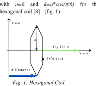
2 2 y d y a ) n / sin( * d y k nak * 2 I H − + − + = π π (1)with n=6 and k=a*cos(π/6) for the
hexagonal coil [8] - (fig. 1).
Y a x is I C u r r e n t d D is ta n c e Z a x is H y F ie ld a
Fig. 1: Hexagonal Coil.
The addition of several coils gives rise to a ripple on the axis. The expression (1) may be expanded in series of equal-ripple functions as Tchebychev polynomials. The position and current may be adjusted to cancel the successive coefficients. So, the axial field will be homogeneous within the high-order terms, which are negligible, provided they decrease in magnitude. Tchebychev polynomials are given by:
Tn(x)=cos(n*arc cos(x)) for -1 ≤ x ≤ 1 (2)
They are orthogonal when integrated over [-1;1] with a weight function (1-x2)–1/2:
( )
(
)
= = ≠ = ≠ = − ∫ − m n 0 0 n m n m 2 / 0 dx x 1 ) x ( T * x T 1 1 2 m n π π (3)As a consequence of this property, it is possible to expand a function f(x) within the range [-1;1] as a serie of Tchebychev polynomials: f(x)= t0+t1*T1(x)+t2*T2(x)+…. (4) Where: ∫ − − 1 1 2 0 dx ) x 1 ( ) x ( f 1 π = t (5) dx ) x 1 ( ) x ( f * ) x ( Tn 2 t 1 1 2 n ∫ − − = π for n≠0 (6)
For an hexagonal coil pair at y = ± d and for a= 1, the field is:
( ) ( )
(
)
( )(
( ))
( )( ) + + + + + − + − + = 2 2 2 2 2 2 d y 1 * d y k 6 / sin * k * I * 12 d y 1 * d y k 6 / si * k * I * 12 Hy n π π (7)If L is the half-length where the ripple has to be minimized, we make the substitution
y=L*x and cosθ=y/L to expand Hy(y,d) over
[-L;L]; expressions (5) and (6) become:
( )
d π1 π H (Lcosθ,d )dθ t 0 y 0 =∫
(8)( )
θ θ θ π π d ) n cos( * ) d , cos L ( H 2 d t 0 y n =∫
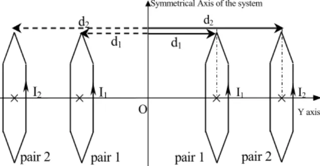
(9)Let’s take a double pair of hexagonal coils as an example (figure 2). By symmetry of the system with respect to the origin, the odd coefficients are cancelled.
d2 d1
I1 I2
pair 1 pair 2 pair 2 pair 1
Symmetrical Axis of the system
O Y axis
d2
d1
I1
I2
Fig. 2: System with two pairs of coils.
By choosing a unity current (I1=1) in
the middle pair of coils, only three parameters must be adjusted: I2, d1 and d2. It
means that we will be able to minimize three even coefficients of the expansion (terms of 2nd, 4th and 6th degree).
B2=1*t2(d1)+I2*t2(d2)
B4=1*t4(d1)+I2*t4(d2)
B6=1*t6(d1)+I2*t6(d2)
B2, B4 and B6 represent the residual error on
the field. We chose to minimize the function
f, sum of the quadratic deviations associated
with the Tchebychev polynomials of order
2,4, and 6.
f(I2,d1,d2)=B22+B42+B62 (10)
2-2 Application to the L coils
To obtain the equal-ripple allowed on the length expected, the above mentioned method leads to install 7 pairs of coils (see further down). It means that 13 parameters have to be adjusted: 6 currents (I2,…I7) and
7 distances (d1,d2,…d7). We must obtain the
simultaneous cancellation of the 13 coefficients, B2 to B26:
B2=1*t2(d1)+I2*t2(d2)+I3*t2(d3)+I4*t2(d4)+I5*t2(d5)
+I6*t2(d6)+I7*t2(d7)
M
B26=1*t26(d1)+I2*t26(d2)+I3*t26(d3)+I4*t26(d4)
+I5*t26(d5)+I6*t26(d6)+I7*t26(d7)
To find the optimum, we have to minimize the "target” function f:
f(I2,..,I7,d1,...,d7)=B22+B42+...+B262 (11)
A direct use of traditional optimization algorithms for a system of nonlinear equations with 13 unknown is not obvious and it takes too much computation time. Moreover the convergence zone is very restricted for such a set of parameters.
To improve the solution, we will proceed in two steps. In a first step, starting from an initial set of parameters (d1,……d7)
we can notice that half of the coefficients can be determined by solving in a linear way the system: B2=B4=B6=B8=B10=B12=0 (12) i. e. − = + + + + + − = + + + + + − = + + + + + − = + + + + + − = + + + + + − = + + + + + ) d ( t ) d ( t * I ) d ( t * I ) d ( t * I ) d ( t * I ) d ( t * I ) d ( t * I ) d ( t ) d ( t * I ) d ( t * I ) d ( t * I ) d ( t * I ) d ( t * I ) d ( t * I ) d ( t ) d ( t * I ) d ( t * I ) d ( t * I ) d ( t * I ) d ( t * I ) d ( t * I ) d ( t ) d ( t * I ) d ( t * I ) d ( t * I ) d ( t * I ) d ( t * I ) d ( t * I ) d ( t ) d ( t * I ) d ( t * I ) d ( t * I ) d ( t * I ) d ( t * I ) d ( t * I ) d ( t ) d ( t * I ) d ( t * I ) d ( t * I ) d ( t * I ) d ( t * I ) d ( t * I 1 12 7 12 7 6 12 6 5 12 5 4 12 4 3 12 3 2 12 2 1 10 7 10 7 6 10 6 5 10 5 4 10 4 3 10 3 2 10 2 1 8 7 8 7 6 8 6 5 8 5 4 8 4 3 8 3 2 8 2 1 6 7 6 7 6 6 6 5 6 5 4 6 4 3 6 3 2 6 2 1 4 7 4 7 6 4 6 5 4 5 4 4 4 3 4 3 2 4 2 1 2 7 2 7 6 2 6 5 2 5 4 2 4 3 2 3 2 2 2
This 6 equations and 6 unknowns (I2,...,I7)
system is solved in a traditional way, by matrix inversion. We get the current values for which 6 coefficients (B2 to B12) are
cancelled. Half of the problem is already solved very easily and the “target” function remaining to be optimized is now:
f(d1,...,d7) = B142+....+B262 (13)
We obtain the optimal values for (d1,...d7) by minimizing expression (13) with
available standard algorithm (optimization toolbox MatLab). Furthermore, the t2n(d)
coefficients are more efficiently calculated by using a Gauss-Legendre quadrature approximation instead of integrating expression (9) [9].
There is only one optimal solution; we call “the canonical solution”. This solution is the best one because any deviation from
the theoretical results does not change in a significant way the field homogeneity.
As mentioned above, in the first step, we have to start with an initial set for (d1…dn). With a low number of coils, the
choice for this initial set is not critical and we have a large length range available that gives us the canonical solution. When the coil number is increasing, some local minimum due to a bad set could give unstable solutions and it is not realistic to directly optimize a system with 7 pairs of coils. We first apply this method to a double pair of coils whose the results are used as “initial set” for 3 pairs of coils, and so on, until the imposed ripple is reached.
The progression toward the result is summarized in table 1.
Number of pair of coils - L=2.65
2 3 4 5 6 7 D1 0.8678 0.58 0.4352 0.3482 0.2782 0.2371 D2 2.4133 1.665 1.2731 1.0277 0.8273 0.7061 D3 2.6965 2.0408 1.6643 1.3572 1.1637 D4 2.8754 2.2667 1.8657 1.61 D5 3.0075 2.3793 2.0495 D6 3.0763 2.511 D7 3.176
Table 1: Results from 2 to 7 pair of coils.
With 7 pair of coils, we got the expected uniformity (<2 10-4) on the maximum length (L=2.65). The distances d1
to d7 are in normalized units, compared to
the radius of the circle inscribed within the hexagon (a=1). Fig.3 represents these results and shows how it is possible, step by step to found the canonical solutions when increasing the number of coils.
Number of pair of coils
Coil’s Position (d) 1 2 3 4 2 4 5 6 7 3
Fig. 3: Coils position (normalized unit).
The parameters (7 distances and 6 currents) of the LMMCF simulator corresponding to the optimal (canonical) solution are given in table 2 (normalized units).
Pair N° 1 2 3 4 5 6 7
Distance 0.237 0.706 1.164 1.61 2.05 2.511 3.176
Current 1.000 0.981 0.959 0.942 0.950 1.098 2.378
Table 2: Canonical Solution for LMMCF
(7 currents and 7 distances, L=2.65).
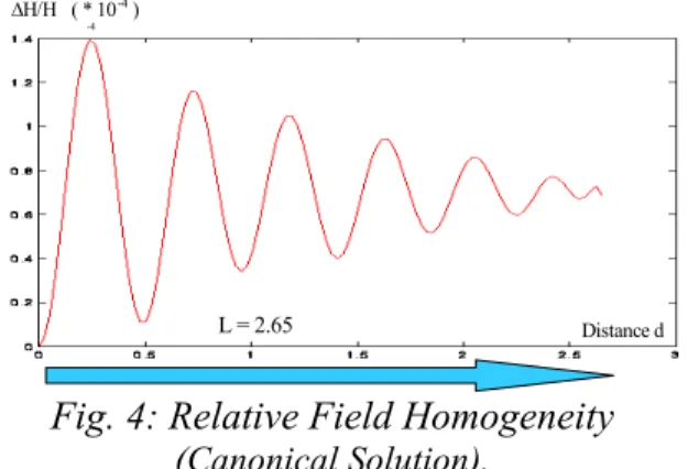
Fig.4 gives the relative homogeneity of the field along the Y axis.
-4
∆H/H ( * 10-4
)
Distance d
L = 2.65
Fig. 4: Relative Field Homogeneity
(Canonical Solution).
L is the half-optimization length from the origin. Vertical axis represents the relative homogeneity variation from the origin.
N.B For a set of n coils, the canonical solution leads to n field oscillations, regularly decreasing over the optimization length. This characteristic belongs only to the canonical solution making it a good way to discriminate from sub-optimal solutions.
2-3 Final design
For simplicity and stability, all the coils are connected in series and supplied by a bipolar generator such as only one current has to be controlled. The six inside pairs of coils carry the same number of Amp-turns ; the two end coils are identical but with a different number of Amp-turns. Considering this configuration, only 9 parameters must be adjusted - 2 currents and 7 positions-. Table 3 gives the new parameters of the optimal solution for the final realization:
Pair N° 1 2 3 4 5 6 7
Distance 0.249 0.733 1.219 1.704 2.185 2.658 3.25
Current 1 1 1 1 1 1 2.14
Table 3: Optimal Solution for final realization (2 currents and 7 positions) L=2.65
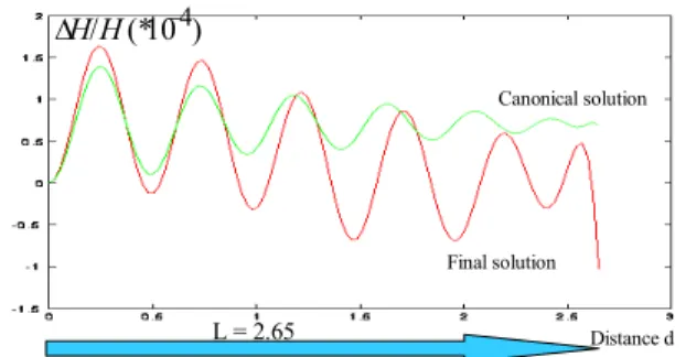
These results are slightly different from canonical solution and the field homogeneity is compared in Fig. 5.
L = 2.65 Distance d Canonical solution Final solution ) 10 (* / −4 ∆ HH
Fig.5: Field homogeneity for the two solutions.
We can notice that the number of oscillations is only six instead of seven, which confirm that this optimal solution is not the canonical solution (previous N.B). However, as we started from the canonical set for (d1,…d7) defined on table2, the field
homogeneity is slightly decreased but the ripple specification is still respected over the required length.
Finally, the longitudinal simulator consists of 14 coils connected in series with the positions and Amp-turns ratio defined in table 3 (standardized units).
3. Vertical and transversal simulator Once the main longitudinal simulator has been determined, we must define the coils set for the two perpendicular directions (vertical and transversal). The basic shape will be the same and consists of several rectangular loops whose length and width are close to those of the building. The structure for V or T simulator is the same, except it’s rotated by 90°, so this enables us to study only one set.
While for the L coil set, the ripple is only optimized along the Y axis, (the off-axis homogeneity then depends of the outer circle radius), for V or T we have to take into account two directions for each one:
along the axis normal to the loop (Z for V and X for T) which define an homogeneity in the vertical median plan parallel to the plane of the loop, on the Y axis.
3-1 Homogeneity in the vertical plane In a first step, let us consider a system with infinite wires. We have to determine
the number of infinite wire pairs, giving us the homogeneity required over the maximum length along the axis in a vertical plane perpendicular to these wires.
Using spherical harmonics [3], we express the field of an infinite wire as a development of the nth derivative in Taylor series about the origin. This development allows optimization of positions and currents for infinite wires in a cross section, by cancellation of even successive derivatives.
Results are given in Fig.6 and table 3. T2, T4 or T6 type means that derivatives are
cancelled up to 2nd, 4th or 6th order. 30° 30° I I 45° 45° 2 * I I I T2 T4 45°
Fig. 6: Disposition of infinite wires in a cross section for vertical field.
Homogeneity of planes Number Conductor
Location I Value ± π/3 1 T2 0.18*R 2 xxxxxxxxxxxxx Xxxxxx ± π/4 √2 T4 0.32*R 3 π/2 1 ± π/5 1 T6 0.42*R 4 ± 2*π/5 0.618
Table 4: Optimal conductor location and Amp-turns vs number of infinite wire pairs
The T4 design has been chosen
because it’s the only one witch allows to use the 45° support for both, vertical and transversal simulator. It needs a ratio 2
between the mid coil current, and the upper and lower ones.
As mentioned earlier, these results come from the optimization using infinite straight conductors. They concern only the homogeneity along the normal axis of the loops and lead to the simplest structure with 3 rectangular coils, as shown in fig. 7.
This elementary layout gives the expected results along the Z axis, however on longitudinal direction Y, the terminal segment effects limit the homogeneous length and they must be taken in account.
x y z
Fig. 7: Elementary structure for the vertical or transversal (rotated by 90°) simulator.
One way to reduce these effects is to split the end segments of median coil into two parts and push back those of side coils. The modified main structure of V simulator with horse saddle shape for each coil, is represented in Fig. 8 B' C' D' A' D" A" C" B" D A B C Median V coil Lower coil Upper coil D' A' D" A" B' C' C" B" x y z
Fig. 8: Modified V simulator structure with horse saddle.
Choosing a horse saddle shape for the coils, brings up several advantages:
access in the simulator is much easier than with a straight connection in the horizontal plane, especially for median coil.
field homogeneity on median longitudinal axis is also increased.
moreover, with hexagonal ends, the same frame as the longitudinal simulator is usable and both coil sets (V ant T) will be fitted with L coils.
3-2 Longitudinal Y axis optimization Although horse saddle shape with hexagonal ends provides a better homogeneity than rectangular loops, this partial improvement is not sufficient to meet the specifications along the Y axis.
To increase significantly this homogeneity length, we install additional
coils similar to the main one, as shown in Fig. 9.
Main coils
Upper set of coils
Median set of coils
d1 d2 d3 3 * 2 I 3 I 2 * 2 I 1 * 2 I 2 I I1 D A D' A'
Fig. 9: 1/4 of the complete V simulator.
These additional coils produce a ripple along the Y axis. By adjusting the positions and the Amp-turns of each coil with the Tchebychev polynomial expansion method, we minimize this ripple.
The system, with 5 unknown parameters -2 currents and 3 positions- is solved in the same way as for the longitudinal simulator. Only expression (7) for the field is modified to the right one corresponding to a multi segments coil [8].
The results of this optimization are given in table 5: I1 I2 I3 d1 d2 d3 Median coil 1 2,358 163,5 0,846 1,661 3,558 Sym. coils 1 2,471 177,4 0,819 1,622 3,554 Positions Current(A/T)
Table 5: Optimal solutions for vertical simulator (L=2).
The geometry of the upper and lower ends is not the same as the median one, so we obtain two sets of positions and currents. There is only a slight difference between the two sets. In order to simplify the construction, we took the average of the 2 values, after verifying it had no effect on the overall homogeneity.
4. Theoretical and experimental results. The components of the local earth field are:
HL:20700nT; HV: 40400nT and HT<100nT
For hexagonal coils with 4m sides (a=4) and to create a field of ± 50 000 nT, the final parameters for the field simulator are summarized on the tables 6 and 7, respectively for L and V coils.
Pair N° 1 2 3 4 5 6 7 Distance
(in meter) 0.977 2.930 4.878 6.818 8.740 10.632 12.977
Amp Turn 14 14 14 14 14 14 30
Table 6: L simulator (real units with a=4).
For the V simulator, the upper and lower coils (or side coils for T) are located at 45°, on the side of the hexagon, so the distance to be considered is 3,69m (a’=3,69)
d3 fixed
R=3,69 I1 I2 I3 d1 d2 d3
Practical
Design 1 2,415 170,59 3,074 6,060 13,134
Distance for Pair N° Currant(A/T)
Table 7: V simulator(real units for a’=3,69)
4-1 Field verification
Once the geometry and the Amp-turns of the simulator have been determined, an another program using the Biot and Savart law, computes the field created by each axis (or by the complete three-axes simulator).
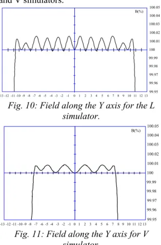
As an example, Fig. 10 and 11 give the results for the field along Y axis, for L and V simulators. B(%) 100 99.99 99.98 99.97 99.96 99.95 100.01 100.02 100.03 100.04 100.05 -13 -12 -11 -10 -9 -8 -7 -6 -5 -4 -3 -2 -1 0 1 2 3 4 5 6 7 8 9 10 11 12 13
Fig. 10: Field along the Y axis for the L simulator. B(%) 100 99.99 99.98 99.97 99.96 99.95 100.01 100.02 100.03 100.04 100.05 -13 -12 -11 -10 -9 -8 -7 -6 -5 -4 -3 -2 -1 0 1 2 3 4 5 6 7 8 9 10 11 12 13
Fig. 11: Field along the Y axis for V simulator.
The residual ripple meets our requirements, i. e. lower than 2.10-4.
The designed homogeneity along all the axes of this three-axial simulator (9 terms) is summarized in table 8.
Simulator Y Axis X Axis Z Axis
L 1% on 23 m < 3*10-4 on 21 m 1% on 4 m < 3*10-4 on 2 m 1% on 4.2 m < 3*10-4 on 2 m V 1% on 18 m < 2*10-4 on 15 m 1% on 3.2 m < 2*10-4 on 1.8 m 1% on 3.6 m < 2*10-4 on 1.8 m T 1% on 18 m < 2*10-4 on 15 m 1% on 3.6 m < 2*10-4 on 1.8 m 1% on 3.2 m < 2*10-4 on 1.8 m Field Homogeneity
Table 8: Field Homogeneity on the 3 axis.
4-2 Measurements
The magnetic simulator has been built in accordance with the geometry defined thanks to this optimization and is now in use.
The first experimental measurements gave excellent results, very close to the predicted one (ripple <2 10-4 on a 15m length )
As an example; Fig. 12 shows the measured field created by the horizontal simulator(L).along the Y axis
5.5 m 5 nT
Fig. 12: Axial homogeneity for L Coils.
This measurement has been done with a fluxgate sensor; fixed on a cart moving along Y axis. We present only a length 5.5 m but the homogeneity is the same over 20 m.
The field created by L coils was close to 20700 nT, such as to compensate horizontal component of local earth field. The measured homogeneity reach 2.3 10-4 (4 nT/20700 nT). 5. Conclusion
An analytical approach to optimize the design of a three-axes magnetic field simulator has been described. This method, using Spherical harmonics and Tchebychev polynomial expansion gives us a flat or an equal-ripple solution we called “canonical solution”.
When increasing the coils number, the program developed is really efficient to minimize this ripple, in order to satisfy given specifications.
Moreover, the complementary program predicting the air coils field in all the space is very useful to check the theoretical results given by the optimization routine.
By applying these tools to our simulator, we obtained the required homogeneity, i.e. lower than 2.10-4, in a large volume (1,6m*1,6m*15m).
The experimental measurements have validated the method and the theoretical results.
We have now a flexible tool, enable us to design any air coils structure, in order to satisfy given criteria.
As a final remark, Tchebychev polynomials method could be taken into account more than it is today for magnetic system design.
Acknowledgment
This works and this project has been supported by the DGA/DCE/GESMA.
B. Barreyres was very helpful in translating the original H.P. Basic software into an up to date Matlab version.
References
[1] LUGANSKY L. B.
"On optimal synthesis of magnetic fields" Journal of Physics, 1,53 (1990)
[2] GARRET M.W.
"Axially symmetric systems for generating an measuring magnetic fields Part I". Applied Physics Journal, Vol. 22, N°9, pp1091-1107 (1951).
[3] ROMEO F. & HOULT D.
"Magnetic field profiling, analyzing and correcting coil design."
Magnetic Resonance in Medicine, Vol.1 p44, 1984
[4] SAUZADE M. and KAN S.
"High resolution nuclear magnetic resonance spectroscopy in high magnetic fields".
Adv. Electron. Phys., p. 1-93 (1973) [5] R.G. CARTER
"Coil System Design for production of uniform magnetic fields".
Proc. IEEE, Vol. 123, N°11 Nov.1976 pp1279-1283.
[6] LEIFER M.
"R F solenoid with extended equiripple field profile". Journal of Magnetic Resonance, Ser. A 105 p.1-2 (1993).
[7] BONGIRAUD J-P., CAUFFET G., DURET D., JEANDEY C.
"The Magnetic Metrology Laboratory for Low Field in Grenoble". Electromagnetic Silencing Symposium-95 (EMSS-95)-Bergen (Norway)- OTAN Conference. [8] E. DURAND
"Magnétostatique". Edition Masson 1966 [9] PRESS W.H. et FLANNERY B. P.
Numerical Recipies, Cambridge ed., p.147 (1986).