Multiple triangulation analysis: application to determine the velocity of 2-D structures

HAL Id: hal-00318221

https://hal.archives-ouvertes.fr/hal-00318221

Submitted on 22 Nov 2006

HAL is a multi-disciplinary open access

archive for the deposit and dissemination of

sci-entific research documents, whether they are

pub-lished or not. The documents may come from

teaching and research institutions in France or

abroad, or from public or private research centers.

L’archive ouverte pluridisciplinaire HAL, est

destinée au dépôt et à la diffusion de documents

scientifiques de niveau recherche, publiés ou non,

émanant des établissements d’enseignement et de

recherche français ou étrangers, des laboratoires

publics ou privés.

Multiple triangulation analysis: application to determine

the velocity of 2-D structures

X.-Z. Zhou, Q.-G. Zong, J. Wang, Z. Y. Pu, X. G. Zhang, Q. Q. Shi, J. B. Cao

To cite this version:

X.-Z. Zhou, Q.-G. Zong, J. Wang, Z. Y. Pu, X. G. Zhang, et al.. Multiple triangulation analysis:

application to determine the velocity of 2-D structures. Annales Geophysicae, European Geosciences

Union, 2006, 24 (11), pp.3173-3177. �hal-00318221�

www.ann-geophys.net/24/3173/2006/ © European Geosciences Union 2006

Annales

Geophysicae

Multiple triangulation analysis: application to determine the

velocity of 2-D structures

X.-Z. Zhou1,2, Q.-G. Zong3,2, J. Wang1, Z. Y. Pu1, X. G. Zhang1, Q. Q. Shi2, and J. B. Cao2 1_{Institute of Space Physics and Applied Technology, Peking University, Beijing 100871, China} 2_{Key Laboratory for Space Weather, Chinese Academy of Sciences, Beijing 100080, China} 3_{Center for Atmospheric Research, University of Massachusetts, Lowell, MA 01854, USA}

Received: 15 June 2006 – Revised: 7 September 2006 – Accepted: 13 October 2006 – Published: 22 November 2006

Abstract. In order to avoid the ambiguity of the

applica-tion of the Triangulaapplica-tion Method (multi-spacecraft timing method) to two-dimensional structures, another version of this method, the Multiple Triangulation Analysis (MTA) is used, to calculate the velocities of these structures based on 4-point measurements. We describe the principle of MTA and apply this approach to a real event observed by the Clus-ter constellation on 2 October 2003. The resulting velocity of the 2-D structure agrees with the ones obtained by some other methods fairly well. So we believe that MTA is a reli-able version of the Triangulation Method for 2-D structures, and thus provides us a new way to describe their motion.

Keywords. Magnetospheric physics (Magnetospheric

con-figuration and dynamics; Solar wind-magnetosphere interac-tions; Instruments and techniques)

1 Introduction

In order to study the motion of various 2-D structures, sev-eral tools have been developed based on in-situ data from single or multiple satellites. Some of the most widely-used examples are: Spatio-temporal Difference, or STD method (Shi et al., 2006), DeHoffmann-Teller analysis (in detail, see Khrabrov and Sonnerup, 1998), and the Triangulation Method, also referred to as the “timing method” (Russell et al., 1983; Harvey, 1998).

The STD method assumes that the temporal change of the magnetic field, observed by the spacecraft, is only caused by the structure motion, which leads to a set of difference equa-tions. By solving these equations, the velocities can be de-termined point by point. It should be noted that this method can be applied to 1-D, 2-D or 3-D structures.

Correspondence to: Z. Y. Pu

(zypu@pku.edu.cn)

On the other hand, the DeHoffmann-Teller analysis was originally suggested to calculate the velocity of 1-D struc-tures, such as current layers, by seeking a reference frame in which the mean square of the electric field is as small as possible. Khrabrov and Sonnerup (1998) further applied this analysis to 2-D cases, to calculate the frame velocity perpen-dicular to the invariant direction.

The Triangulation Method was also developed initially for 1-D structures, and makes use of the time differences be-tween four spacecraft encountering the same planar struc-ture, in order to calculate its normal direction along with the normal component of the velocity (Russell et al., 1983). It should be noted that due to the relative complexity of the 2-D structures, the application of this method to the 2-D structure is less successful, with difficulties in the determination of the time differences.

In many calculations for 2-D cases, one single character-istic contour plane (such as Bz=0, et cetera) is selected as the signal to judge the time differences (e.g. Eastwood et al., 2005). However, the different signals selected often corre-spond to distinct timing consequences and thus lead to dif-ferent velocities, and it is usually hard to tell why one should select a certain signal instead of another when performing the timing analysis. As a modified version, the time differ-ences can be determined by maximizing the cross-correlation function between the magnetic profiles observed by different satellites (e.g. Fear et al., 2005). However, unlike 1-D cases, the cross-correlation peak is often less clear, and the max-imum value is also much lower. In some of the cases, the time durations of the structure traversal for different satel-lites are shown to be different, which makes it even harder to precisely determine the time differences.

In this paper, we make use of the Multiple Triangula-tion Analysis (Zhou et al., 2006) as another version of the Triangulation Method, to calculate the velocity of the two-dimensional structures. As an example, this approach is also applied to Cluster data and the resulting velocity is compared

3174 X.-Z. Zhou et al. : Multiple triangulation analysis

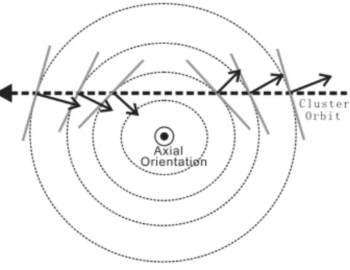
Fig. 1. Sketch of the Cluster constellation traversing a 2-D structure. The set of magnetic contour planes are represented by the dashed circles and the normal directions of these planes are the solid ar-rows. All of these arrows are shown to be perpendicular to the axial orientation of the 2-D structure.

with those obtained by other methods to test the accuracy of the MTA technique.

2 Method

The Multiple Triangulation Analysis was initially developed to obtain the main orientation of 2-D structures, e.g. mag-netic flux ropes (Zhou et al., 2006). Selecting a series of magnetic field magnitudes as the signals, the Triangulation Method can be applied to the 2-D structures for several times, each time with a resulting speed along a certain normal direc-tion. Figure 1 sketches the orbit of the Cluster constellation (the dashed arrow) traversing a 2-D structure. During this traversal, the constellation penetrates a set of magnetic con-tour planes (the dashed circles). Although the shapes of these contour planes may be more complicated, their normal direc-tions (solid arrows) should be basically contained within the cross-section plane and thus perpendicular to the axial orien-tation of the 2-D structure.

These normal directions N(m)(m=1, M), along with the

normal speeds V(m), are now put into the MTA calculation to obtain the the axial orientation H, as the direction “most perpendicular” to these normals, by the minimization of

σ2= 1 M M X m=1 |N(m)·H|2,

which leads to an eigenproblem of a symmetric matrix L:

Lµν = hN(m)µ N(m)ν i, (1) where the subscripts µ, ν=1,2,3 denote the Cartesian com-ponents of the vector N(m)along the X, Y, Z directions, re-spectively. One of the three eigenvectors of L, with the small-est eigenvalue, can be treated as the axial orientation of the 2-D structure (for a more detailed analysis and error estima-tion, see Zhou et al., 2006).

On the other hand, if the structure does not change its con-figuration significantly during the analyzed time interval, the set of normal speeds V(m) can be treated as the components of the structure velocity along their corresponding normal di-rections, i.e. VS·N(m)=V(m). Here VS denotes the structure velocity. In practice, this velocity can be obtained by the minimization of D(VS) = 1 M M X m=1 |VS· N(m)−V(m)|2. (2)

A least-squares approach can be used to determine this veloc-ity. After a straightforward analysis, the minimization prob-lem leads to the linear equation

L · VS = hV(m)·N(m)i, (3) where the brackets h i represent an averaging over the whole data set, and the symmetric matrix L is defined as (1). There-fore, the solution of Eq. (3), VS=L−1·hV(m)·N(m)i, would be the optimal estimation of the structure velocity.

Since we are discussing the velocity of a 2-D structure, it should be noted that the resulting structure velocity com-ponent along the axial orientation is less meaningful. Any arbitrary velocity component along H can be added to the resulting structure velocity with little change in the value of V·N(m), due to the perpendicular properties between the axial orientation and each magnetic contour normal, by definition. So it is natural to set the axial velocity equal to zero. The axial orientation (H1, H2, H3), as was discussed before, is

es-timated as the eigenvector of the matrix L with the smallest eigenvalue. Then we can simply remove the axial compo-nent, thereby obtaining transversal velocity.

An alternative way to obtain the velocity is based on the following constraint:

H1VS1+H2VS2+H3VS3=0,

so that one of the velocity components, say VS3, can be ex-pressed as the function of the other two components. Thus, the minimization of (2) becomes the equation of:

K · V∗_S = hV(m)·H3·N(m)∗i (4)

instead of Eq. (3). Here the asterisk denotes the first two components of the certain vector, and the 2×2 matrix K is defined as:

Kµν =N(m)µ ·(N (m)

ν H3−N(m)₃ Hν),

where µ, ν=1, 2 corresponds to the Cartesian X and Y com-ponents. The solution of Eq. (4) would provide us the first two components of the structure velocity. Following the con-straint that the velocity is perpendicular to the structure’s ax-ial orientation, the Z component of the velocity can also be obtained.

There are two error sources in the MTA velocity calcula-tion: the systematic parts and the random ones. The system-atic errors are mostly produced by the nonplanar properties

0 20 40 60 80 100 0 4 8 12 16 20

X / R

R / d

(a)

(b)

Fig. 2. The error range obtained by the set of MTA tests, selecting 10 contour planes within the structure as the signals. The bootstrap procedure is further applied in each of the MTA tests to display the effect of quantization errors. The difference between the modeled “true” velocity and the MTA velocity, divided by the “true” velocity, can be defined as the error. (a) The error versus flux rope radius R (normalized to d=400 km) in a certain type of Cluster trajectory with X (the constellation’s closest distance to the axis) of 0.707 R. (b) The error dependency on X, which is normalized to the structure radius R), when R is fixed to be 30 times greater than the satellite separation d.

of the magnetic contour planes within the structure, while the random ones may occur because of the quantization effect in applying the timing method.

In order to estimate the error range of the MTA veloc-ity, we simulate a number of 2-D structures with different sizes and make the Cluster constellation cross it along dif-ferent paths. The quantization errors in the determination of traversal times (randomized for each satellite, with the maximum error of 0.08 s) are also taken into account in each simulation, using the bootstrap procedure (e.g. Kawano and Higuchi, 1995; Sonnerup and Scheible, 1998).

For simplicity, the cross-section of the 2-D structure is set to be circular in the xy-plane, and the z-direction-orientated structure is moving with the velocity of 200 km·s−1 along the x-direction. The formation of Cluster is set to be a regu-lar tetrahedron, with the separation of 400 km between each satellite pair. Selecting 10 contour planes as the signals, the MTA technique can be applied on each simulated cross-ing, and the difference between the resulting velocity and the “true” one can be treated as the error in the simulation. The error shows strong dependencies on both the structure ra-dius R and the constellation crossing path (characterized by the closest distance X from the constellation to the structure axis), as is displayed in Fig. 2.

Figure 2a shows the error dependency on the radius of the 2-D structure, with a fixed constellation trajectory of

X/R=0.707. For the cases with the spacecraft separation

to be comparative to the scale of the structure, the error is large because the magnetic contour planes are no longer pla-nar, which violates the basic assumption of the Triangulation Method. 40 50 60 70 80 90 17 18 19 20 21 22 23 24 Time (Second) B total (nT) 40 50 60 70 80 90 −10 −5 0 5 10 15 20 Time (Second) B z (nT) C1 C2 C3 C4

Fig. 3. A 2-D structure observed by FGM/Cluster on 2 October 2003, 00:46:40 UT to 00:47:30 UT. (Left panel) Magnetic strength (Right panel) Bzcomponents, as the function of time (both 6-s slid-ing averages at 0.2-s resolution).

It can be clearly seen from Fig. 2b that the MTA ve-locity error is highly dependent on the path of the Cluster constellation, which is typically less than 4% in the region of 0.2 R<X<0.9 R. For the X>0.9 R cases, the relatively larger systematic errors are caused by the skimming motion over the 2-D structure. On the other hand, for the X<0.2 R cases, for which the path is very close to the structure axis, the errors are mainly random ones, which should be pro-duced by the ambiguity in the determination of the axial ori-entation (see the error estimation part of Zhou et al., 2006). However, because of the approximate parallelism of the set of normal directions in these cases, the resulting minimum eigenvalue λ3should be very close to the intermediate one

λ2. So the relatively smaller value of λ2/λ3can provide us

with a warning of the invalidation of the MTA technique on the estimation of both axial orientation and traversal velocity.

3 Applications

On 2 October 2003, the Cluster constellation was in the mag-netotail observing a 2-D structure. This event was originally discovered by Eastwood et al. (2005), as an example of a flux rope-type structure moving earthward. The authors assumed that the surface Bz=0 is planar on the scale of the space-craft tetrahedron and by applying the timing method, found a speed of 140±13 km·s−1 along the direction of (0.778, 0.595, 0.158) GSM.

Now we apply the Multiple Triangulation procedure to this data set as a comparison, using magnetic field data (FGM data) (Balogh et al., 1997). Figure 3 shows the events in the time interval of 00:46:40 UT–00:47:30 UT: |B| in the left panel, and Bzin the right panel. Note that the high-frequency fluctuations were removed with a sliding average procedure

3176 X.-Z. Zhou et al. : Multiple triangulation analysis −1 0 1 −1 0 1 −1 0 1 Y X Z −1 −0.5 0 0.5 1 −1 −0.5 0 0.5 1 L M

Fig. 4. The MTA analysis on the event during 00:46:40 UT to 00:47:30 UT. The blue lines show the normal directions obtained by the Triangulation method as the first step of MTA, and the red lines are the three eigenvectors of the corresponding matrix. The green circle represents the cross-section plane of the flux rope, basically containing all of the blue lines, while the red line perpendicular to the green circle suggests the flux rope orientation. The left box is in GSM, while the right one is in the LMN coordinate system defined by three eigenvectors.

(Haaland et al., 2004). Here we use a sliding window of 6 s, with a time resolution of 0.2 s, and apply linear inter-polation between each consecutive measurements. Then we select a set of magnetic field values as the signals, shown as magenta dashed lines in the left panel of Fig. 3, to obtain 23 normal directions and speeds using the timing method. The 23 directions, displayed as blue lines in Fig. 4, thus lead us to the calculation of the matrix L and its three eigenval-ues and eigenvectors (shown as red lines). The eigenvector (0.289, −0.570, 0.769) GSM with the smallest eigenvalue (λ2/λ3=66.6) should be, in principle, perpendicular to all of

the 23 normals, as the estimated axial orientation of the 2-D structure. The large separation between eigenvalues further suggests that the statistical error of the estimated axial orien-tation is as small as 1.5 degree (see Zhou et al., 2006). As can be clearly seen in Fig. 4, all of the 23 normals are very well confined in the plane (green circle) composed by the other two eigenvectors.

The estimated axial orientation can now be used to calcu-late the matrix K. Solving Eq. (4) thus leads to the calcula-tion of a structure velocity of around (95.19, 100.03, 38.28), i.e. the speed of 143.3±2.4 km·s−1 along the direction of GSM (0.664, 0.698, 0.267), with an angular error of 2.0 de-gree.

All of the 23 velocity vectors are plotted together (as blue lines) in the LMN coordinate system, defined by the L eigen-vectors, in the left panel of Fig. 5. As was discussed before, the LM plane of this coordinate system can be treated as the cross-section plane of the certain 2-D structure. The struc-ture velocity, obtained by the least-squares procedure, is also shown in the figure, as the red line. Since the 23 velocity vectors are believed to be the components of the structure

−20 20 60 100 140 −50 −10 30 70 110 V SL (kms −1 ) V_SM (kms−1) 0 40 80 120 160 0 40 80 120 160 V_S N(m) (kms−1) V (m) (kms −1 ) (0,0)

Fig. 5. (Left panel) The set of velocities V(m)·N(m)as blue lines and the structure velocity VSas the red line in the LMN coordinate system defined by three eigenvectors. (Right panel) Scatter plot of the speed V(m) as the function of VS·N(m). The correlation coefficient is 0.995.

velocity, all of the vector-end points should be theoretically located in the circle with the structure velocity as the diame-ter, as is also very clearly seen in the figure.

To give an impression of the precision of the obtained ve-locity, the two speeds, VS·N(m)and V(m), are plotted against each other, in the right panel of Fig. 5. The correlation be-tween these two speeds is high, with the correlation coeffi-cient of 0.995. Then we may go back to the result obtained by Eastwood et al. (2005), with the speed of 140±13 km·s−1 along the direction of GSM (0.778, 0.595, 0.158). However, in their timing analysis, only one signal is selected (the ma-genta dashed line in the right panel of Fig. 3). Although their resulting velocity seems to be similar with the MTA veloc-ity, it should be noted that this velocity cannot be treated as the structure velocity based on our discussion. Instead, the velocity is one component of the structure velocity along the normal direction of the Bz=0 plane. Therefore, the velocity (shown in the left panel of Fig. 5 as the black line) should play the same role as the 23 normal velocities discussed be-fore. The vector-end point of this black line is found to be precisely located in the green circle, similar to the 23 vector-end points. Actually, the component of−→VSin this direction is 139.6±2.3 km·s−1, which agrees with their result extremely well.

As another comparison, the STD method is also applied in this case. During this time period, the STD velocity is rather stable, with the mean speed of 152.8 km·s−1along the direc-tion of GSM (0.706, 0.675, 0.213). The estimated speed is 9.5 km·s−1_{larger than the MTA result and the angular}

devi-ation between them is only 4.2 degrees. Their similarities, in some sense, confirm the reliability and consistency of both the MTA and STD methods.

DeHoffmann-Teller analysis, as a classical technique to obtain the velocity of structures, should be also applied to examine the precision of MTA approach. However, in this 2-D structure crossing, the time interval is fairly short, which invalidates the VH T result.

4 Summary

In order to avoid the ambiguity in the application of the Tri-angulation Method to 2-D structures, the approach of the Multiple Triangulation Analysis is presented as a new ver-sion of Triangulation Method. While the traditional Triangu-lation Method can only provide one single component of the structure velocity, the MTA approach makes use of the set of velocity components obtained by the traditional method to calculate both the axial orientation and the optimal structure velocity. Real Cluster data sets are used and comparisons with other methods are also made to prove the precision of this approach. In addition, the MTA approach can have the ability to provide more accurate results for future missions with more than 4 satellites.

Acknowledgements. The authors thank J. P. Eastwood of Univer-sity of California at Berkeley for many helpful discussions. We are also grateful to K.-H. Glassmeier of Technische Universitat Braun-schweig for providing the high resolution Cluster/FGM data. This work is supported by NSFC project 40528005, 40390152 and the International Collaboration Research Team Program of the Chinese Academy of Sciences.

Topical Editor I. A. Daglis thanks J. Birch and another referee for their help in evaluating this paper.

References

Balogh, A., Dunlop, M. W., Cowley, S. W. H., Southwood, D. J., Thomlinson, J. G., Glassmeier, K.-H., Musmann, G., Lu¨hr, H., Buchert, S., Acuna, M. H., Fairfield, D. H., Slavin, J. A., Riedler, W., Sachwingenschuh, K., and Kivelson, M. G.: The Cluster Magnetic Field Investigation, Space Sci. Rev., 79, 65–91, 1997. Eastwood, J. P., Sibeck, D. G., Slavin, J. A., Goldstein, M. L.,

Lavraud, B., Sitnov, M., Imber, S., Balogh, A., Lucek, E. A., and Dandouras, I.: Observations of multiple X-line structure in the Earth’s magnetotail current sheet: A Cluster case study, Geophys. Res. Lett., 32, L11 105, doi:10.1029/2005GL022509, 2005.

Fear, R. C., Fazakerley, A. N., Owen, C. J., and Lucek, E. A.: A survey of flux transfer events observed by Cluster during strongly northward IMF, Geophys. Res. Lett., 32, L18 105, doi:10.1029/2005GL023811, 2005.

Haaland, S., Sonnerup, B. U. O., Dunlop, M. W., Balogh, A., Georgescu, E., Hasegawa, H., Klecker, B., Paschmann, G., Puhl-Quinn, P., Reme, H., Vaith, H., and Vaivads, A.: Four-spacecraft determination of magnetopause orientation, motion and thick-ness: comparison with results from single-spacecraft methods, Ann. Geophys., 22, 1347–1365, 2004,

http://www.ann-geophys.net/22/1347/2004/.

Harvey, C. C.: Spatial Gradients and the Volumetric Tensor, in: Analysis Methods for Multi-spacecraft Data, edited by: Paschmann, G. and Daly, P., pp. 307–322, ISSI/ESA, Nether-lands, 1998.

Kawano, H. and Higuchi, T.: The bootstrap method in space physics: Error estimation for minimum variance analysis, Geo-phys. Res. Lett., 22, 307–310, 1995.

Khrabrov, B. V. and Sonnerup, B. U. O.: DeHoffmann-Teller Anal-ysis, in: Analysis Methods for Multi-spacecraft Data, edited by: Paschmann, G. and Daly, P., pp. 221–248, ISSI/ESA, Nether-lands, 1998.

Russell, C. T., Mellott, M. M., Smith, E. J., and King, J. H.: Mul-tiple Spacecraft Observations of Interplanetary Shocks: Four Spacecraft Determination of Shock Normals, J. Geophys. Res., 88, 4739–4748, 1983.

Shi, Q. Q., Shen, C., Dunlop, M. W., Pu, Z. Y., Zong, Q.-G., Liu, Z. X., Lucek, E., and Balogh, A.: Motion of observed structures calculated from multi-point magnetic field measure-ments: Application to Cluster, Geophys. Res. Lett., 33, L08 109, doi:10.1029/2005GL025073, 2006.

Sonnerup, B. U. O. and Scheible, M.: Minimum and Maximum Variance Analysis, in: Analysis Methods for Multi-spacecraft Data, edited by: Paschmann, G. and Daly, P., pp. 185–220, ISSI/ESA, Netherlands, 1998.

Zhou, X.-Z., Zong, Q.-G., Pu, Z. Y., Fritz, T. A., Dunlop, M. W., Shi, Q. Q., Wang, J., and Wei, Y.: Multiple Triangulation Analy-sis: Another Approach to Determine the Orientation of Magnetic Flux Ropes, Ann. Geophys., 24, 1759–1765, 2006,