Distributed optimization and market analysis of networked systems

(1)

Distributed Optimization and Market Analysis

of Networked Systems

by

Ermin Wei

B.S., Computer Engineering

B.S., Mathematics

B.S., Finance

Minor in German Language, Literature, and Culture

University of Maryland, College Park (2008)

M.S., Electrical Engineering and Computer Science

Massachusetts Institute of Technology (2010)

Submitted to the Department of Electrical Engineering and Computer

Science

in partial fulfillment of the requirements for the degree of

Doctor of Philosophy in Electrical Engineering and Computer Science

at the

MASSACHUSETTS INSTITUTE OF TECHNOLOGY

September 2014

c

○ Massachusetts Institute of Technology 2014. All rights reserved.

Author . . . .

Department of Electrical Engineering and Computer Science

August 29, 2014

Certified by . . . .

Asu Ozdaglar

Professor

Thesis Supervisor

Accepted by . . . .

Leslie Kolodziejski

Chairman, Department Committee on Graduate Theses

(2)

(3)

Distributed Optimization and Market Analysis

of Networked Systems

by

Ermin Wei

Submitted to the Department of Electrical Engineering and Computer Science on August 29, 2014, in partial fulfillment of the

requirements for the degree of

Doctor of Philosophy in Electrical Engineering and Computer Science

Abstract

In the interconnected world of today, large-scale multi-agent networked systems are ubiquitous. This thesis studies two classes of multi-agent systems, where each agent has local information and a local objective function. In the first class of systems, the agents are collaborative and the overall objective is to optimize the sum of local objective functions. This setup represents a general family of separable problems in large-scale multi-agent convex optimization systems, which includes the LASSO (Least-Absolute Shrinkage and Selection Operator) and many other important ma-chine learning problems. We propose fast fully distributed both synchronous and asynchronous ADMM (Alternating Direction Method of Multipliers) based methods. Both of the proposed algorithms achieve the best known rate of convergence for this class of problems, 𝑂(1/𝑘), where 𝑘 is the number of iterations. This rate is the first rate of convergence guarantee for asynchronous distributed methods solving sepa-rable convex problems. For the synchronous algorithm, we also relate the rate of convergence to the underlying network topology.

The second part of the thesis focuses on the class of systems where the agents are only interested in their local objectives. In particular, we study the market interaction in the electricity market. Instead of the traditional supply-follow-demand approach, we propose and analyze a systematic multi-period market framework, where both (price-taking) consumers and generators locally respond to price. We show that this new market interaction at competitive equilibrium is efficient and the improvement in social welfare over the traditional market can be unbounded. The resulting system, however, may feature undesirable price and generation fluctuations, which imposes significant challenges in maintaining reliability of the electricity grid. We first estab-lish that the two fluctuations are positively correlated. Then in order to reduce both fluctuations, we introduce an explicit penalty on the price fluctuation. The penalized problem is shown to be equivalent to the existing system with storage and can be implemented in a distributed way, where each agent locally responds to price. We analyze the connection between the size of storage, consumer utility function prop-erties and generation fluctuation in two scenarios: when demand is inelastic, we can

(4)

explicitly characterize the optimal storage access policy and the generation fluctu-ation; when demand is elastic, the relationship between concavity and generation fluctuation is studied.

Thesis Supervisor: Asu Ozdaglar Title: Professor

(5)

Acknowledgments

The route to a PhD is not an easy one, and completing this thesis would not be possible without all the wonderful people I managed to encounter in my life. First and foremost, I’d like to thank my super supportive and caring thesis advisor, Prof. Asu Ozdaglar. I am very fortunate to have her as my advisor. The numerous meetings we had and even casual hall-way interactions all have shed lights into my life and countless times have guided me out of the dark abyss called, "I’m stuck". Her awesome mentorship, on both personal and professional fronts, has inspired me to become an academician myself, because what I learned here is too valuable to be kept to myself. The interactions I had with my thesis committee members, Prof. Munther Dahleh, Prof. Ali Jadbabaie and Prof. Steven Low, have been all tremendously beneficial. I want to thank them for the time and dedication in helping with the development of the thesis at various stages. I also want to thank my collaborators, Prof. Azarakhsh Malekian, Shimrit Shtern for the stimulating discussions we had and ingenious works they did. I am grateful to Prof. Daron Acemoglu, Prof. Janusz Bialek, Prof. Eilyan Bitar, Dr. Ali Kakhbod, Prof. Na Li, Prof. Sean Meyn, Dr. Mardavij Roozbehani, Prof. Lang Tong, Prof. Jiankang Wang for all the fruitful discussion we had while developing my thesis. My officemates Elie Adam, Prof. Ozan Candogan, Kimon Drakopoulos, Jenny (Ji Young) Lee, Yongwhan Lim, Milashini Nambiar have all been wonderful and especially cool with my office decorations.

I would like to thank my friends at MIT for all the incredible experience we had together. The fun we had and the stories we shared will always be able to warm my heart and put a smile on my face in the future, no matter how much time passes by. A special thank goes to my family for the continuous love and support, always being there for me. The various lessons learned throughout this enriching PhD experience made me a better person and ready for the new roads awaiting.

Last but not least, I would like to thank you our funding agencies: National Science Foundation, Air Force Research Laboratory, Office of Naval Research and MIT Masdar project. Without their generous support, the work could not have been

(6)

(7)

List of Figures

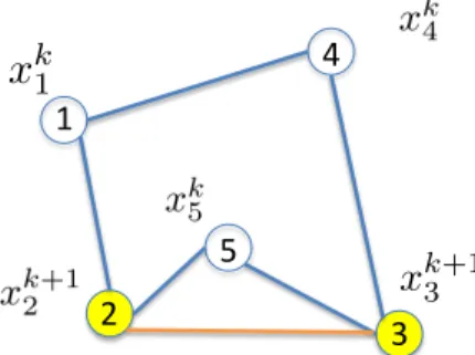
1-1 Reformulation of problem (1.1). . . 18 3-1 Asynchronous algorithm illustration: When edge (2, 3) is active, only

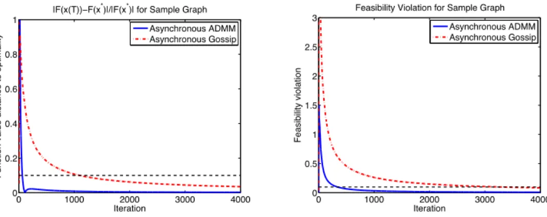
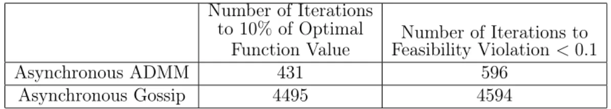
agents 2 and 3 perform update, while all the other agents stay at their previous iteration value. . . 67 3-2 One sample objective function value and constraint violation (𝐴𝑥 = 0)

of both methods against iteration count for the network as in Figure. 3-1. The dotted black lines denote 10% interval of the optimal value and feasibility violation less than 0.1. . . 109 3-3 One sample objective function value and feasibility violation of both

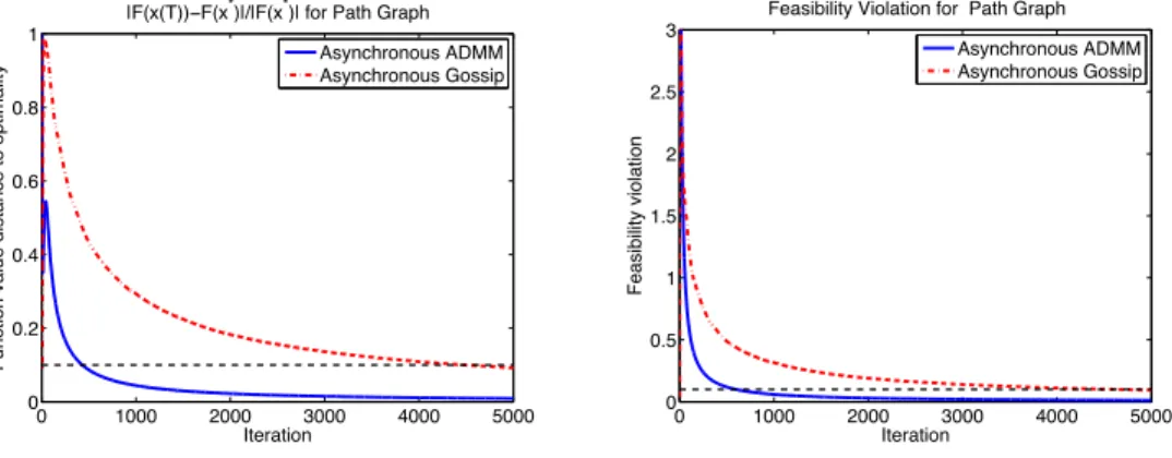
methods against iteration count for the path graph. The dotted black lines denote 10% interval of the optimal value and constraint violation (𝐴𝑥 = 0) less than 0.1. . . 110

(12)

(13)

List of Tables

3.1 Number of iterations needed to reach 10% of optimal function value and feasibility violation less than 0.1 for the network as in Figure. 3-1. 110 3.2 Number of iterations needed to reach 10% of optimal function value

(14)

(15)

Chapter 1 Introduction

1.1 Introduction

In the interconnected world of today, large-scale multi-agent networked systems are ubiquitous. Some examples include sensor networks, communication networks and electricity grid. While the structure of and interaction within these systems may vary drastically, the operations of these networks share some universal characteristics, such as being large-scale, consisting of heterogeneous agents with local information and processing power, whose goals are to achieve certain optimality (either locally or globally).

Motivated by the need to enhance system performance, this thesis studies multi-agent systems in the context of two types of networks. The first type of networks consists of cooperative agents, each of which has some local information, represented as a local (convex) cost function. The agents are connected via an underlying graph, which specifies the allowed communication, i.e., only neighbors in the graph can ex-change information. The system wide goal is to collectively optimize the single global objective, which is the sum of local cost functions, by performing local computation and communication only. This general framework captures many important appli-cations such as sensor networks, compressive sensing systems, and machine learning applications. To improve performance for this type of networks, the thesis will de-velop fast distributed optimization algorithms, both synchronous and asynchronous,

(16)

provide convergence guarantees and analyze the dependence between algorithm per-formance, algorithm parameters and the underlying topology. These results will help in network designs and parameter choices can be recommended.

The second type of systems is where the agents are only interested in their local objective functions. We analyze this type of networks through an example of elec-tricity market. The agents in this system are generators and consumers. One feature that distinguishes electricity market and other markets is that supply has to equal to demand at all times due to the physics of electricity flows.1 _{The traditional electricity}

market treats demand side as passive and inelastic. Thus the generators have to follow precisely the demand profile. However, due to the physical nature of generators, the generation level cannot change much instantaneously. In order to ensure reliability against unanticipated variability in demand, large amount of reserves is maintained in the current system. Both the demand-following nature of generation and large reserve decrease the overall system efficiency level. To improve system efficiency, the new smart grid paradigm has proposed to include active consumer participation, re-ferred to as demand response in the literature, by passing on certain real-time price type signals to exploit the flexibility in the demand. To investigate systematically the grid with demand response integration, we propose a multi-period general mar-ket based model, where the preferences of the consumers and the cost structures of generators are reflected in their respective utility functions and the interaction be-tween the two sides is done through pricing signals. We then analyze the competitive equilibrium and show that it is efficient and can improve significantly over the tra-ditional electricity market (without demand response). To control undesirable price and generation fluctuation over time, we introduce a price fluctuation penalty in the social welfare maximization problem, which enables us to trade off between social welfare and price fluctuation. We show that this formulation can reduce both price and generation fluctuation. This fluctuation penalized problem can be equivalently implemented via introducing storage, whose size corresponds to the penalty

parame-1_{An imbalance of supply and demand at one place can result in black-out in a much bigger area}

(17)

ters. We then analyze the properties and derive distributed implementation for this fluctuation penalized problem. The connections between fluctuation and consumer utility function for both elastic and inelastic demand are also studied.

In the following two sections, we describe the two topics in more depth and outline our main contribution for each part.

1.2 Distributed Optimization Algorithms

1.2.1 Motivation and Problem Formulation

Many networks are large-scale and consist of agents with local information and pro-cessing power. There has been a much recent interest in developing control and optimization methods for multi-agent networked systems, where processing is done locally without any central coordination [2], [3], [5], [68], [69], [70], [36], [71], [6]. These distributed multi-agent optimization problems are featured in many important applications including optimization, control, compressive sensing and signal process-ing communities. Each of the distributed multi-agent optimization problems features a set 𝑉 = {1, . . . , 𝑁 } of agents connected by 𝑀 undirected edges forming an under-lying network 𝐺 = (𝑉, 𝐸), where 𝐸 is the set of edges. Each agent has access to a privately known local objective (or cost) function 𝑓𝑖 : R𝑛 → R, which depends on the

global decision variable 𝑥 in R𝑛 _{shared among all the agents. The system goal is to}

collectively solve a global optimization problem.

min 𝑁 ∑︁ 𝑖=1 𝑓𝑖(𝑥) (1.1) 𝑠.𝑡. 𝑥 ∈ 𝑋.

(18)

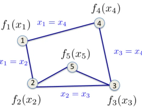
! "# _$# %# &# f2(x2) f1(x1) f3(x3) f4(x4) f5(x5) x1= x2 x3= x4 x1= x4 x2= x3

Figure 1-1: Reformulation of problem (1.1).

problem described as follows:

min 𝑥 𝑁 −1 ∑︁ 𝑖=1 𝑙 ([𝑊𝑖𝑥 − 𝑏𝑖]) + 𝜋 ||𝑥||1,

where 𝑊𝑖 corresponds to the input sample data (and functions thereof), 𝑏𝑖 represents

the measured outputs, 𝑊𝑖𝑥−𝑏𝑖 indicates the prediction error and 𝑙 is the loss function

on the prediction error. Scalar 𝜋 is nonnegative and it indicates the penalty param-eter on complexity of the model. The widely used Least Absolute Deviation (LAD) formulation, the Least-Absolute Shrinkage and Selection Operator (Lasso) formula-tion and 𝑙1 regularized formulations can all be represented by the above formulation

by varying loss function 𝑙 and penalty parameter 𝜋 (see [1] for more details). The above formulation is a special case of the distributed multi-agent optimization prob-lem (1.1), where 𝑓𝑖(𝑥) = 𝑙 (𝑊𝑖𝑥 − 𝑏𝑖) for 𝑖 = 1, . . . , 𝑁 − 1 and 𝑓𝑁 = 𝜋2||𝑥||₁. In

applications where the data pairs (︀𝑊𝑖, 𝑏𝑖)︀ are collected and maintained by different

sensors over a network, the functions 𝑓𝑖 are local to each agent and the need for a

distributed algorithm arises naturally.

Problem (1.2) can be reformulated to facilitate distributed algorithm development by introducing a local copy 𝑥𝑖in R𝑛of the decision variable for each node 𝑖 and

impos-ing the constraint 𝑥𝑖 = 𝑥𝑗 for all agents 𝑖 and 𝑗 with edge (𝑖, 𝑗) ∈ 𝐸. The constraints

represent the coupling across components of the decision variable imposed by the underlying information exchange network among the agents. Under the assumption

(19)

that the underlying network is connected, each of the local copies are equal to each other at the optimal solution. We denote by 𝐴 ∈ R𝑀 𝑛×𝑁 𝑛 _{the generalized edge-node}

incidence matrix of network 𝐺, defined by ˜𝐴 ⊗ 𝐼(𝑛 × 𝑛), where ˜𝐴 is the standard edge-node incidence matrix in R𝑀 ×𝑁_{. Each row in matrix ˜}_{𝐴 represents an edge in}

the graph and each column represents a node. For the row corresponding to edge 𝑒 = (𝑖, 𝑗), we have the ˜𝐴𝑒𝑖 = 1, ˜𝐴𝑒𝑗 = −1 and ˜𝐴𝑒𝑙 = 0 for 𝑙 ̸= 𝑖, 𝑗. For instance, the

edge-node incidence matrix of network in Fig. 1-1 is given by

˜ 𝐴 = ⎡ ⎢ ⎢ ⎢ ⎢ ⎢ ⎢ ⎢ ⎢ ⎢ ⎢ ⎢ ⎢ ⎣ 1 −1 0 0 0 0 1 −1 0 0 0 0 1 −1 0 1 0 0 −1 0 0 1 0 0 −1 0 0 1 0 −1 ⎤ ⎥ ⎥ ⎥ ⎥ ⎥ ⎥ ⎥ ⎥ ⎥ ⎥ ⎥ ⎥ ⎦ ,

and the generalized edge-node incidence matrix is

𝐴 = ⎡ ⎢ ⎢ ⎢ ⎢ ⎢ ⎢ ⎢ ⎢ ⎢ ⎢ ⎢ ⎢ ⎣ 1 −𝐼(𝑛 × 𝑛) 0 0 0 0 𝐼(𝑛 × 𝑛) −𝐼(𝑛 × 𝑛) 0 0 0 0 𝐼(𝑛 × 𝑛) −𝐼(𝑛 × 𝑛) 0 𝐼(𝑛 × 𝑛) 0 0 −𝐼(𝑛 × 𝑛) 0 0 𝐼(𝑛 × 𝑛) 0 0 −𝐼(𝑛 × 𝑛) 0 0 𝐼(𝑛 × 𝑛) 0 −𝐼(𝑛 × 𝑛) ⎤ ⎥ ⎥ ⎥ ⎥ ⎥ ⎥ ⎥ ⎥ ⎥ ⎥ ⎥ ⎥ ⎦ ,

where each 0 is a matrix of size 𝑛 × 𝑛 with all zero elements. The reformulated problem can be written compactly as

min 𝑥𝑖∈𝑋 𝑁 ∑︁ 𝑖=1 𝑓𝑖(𝑥𝑖) (1.2) 𝑠.𝑡. 𝐴𝑥 = 0,

(20)

edge-based reformulation of the distributed multi-agent optimization problem. We also denote the global objective function given by the sum of the local objective function:

𝐹 (𝑥) =

𝑁

∑︁

𝑖=1

𝑓𝑖(𝑥𝑖). (1.3)

This form of objective function, i.e., a sum of local functions depending only on local variables, is called separable.

Due to the large scale nature and the lack of centralized processing units of these problems, it is imperative that the solution we develop involves decentralized compu-tations, meaning that each node (processor) performs calculations independently on the basis of local information available to it and only communicates this information to its neighbors according to the underlying network structure. Hence, the goal in this part of the thesis is to develop distributed optimization algorithm for problem (1.1) with provable convergence and rate of convergence guarantees for large-scale systems.

The distributed algorithms we develop will utilize the parallel processing power inherent in the system and can be used in more general parallel computation settings where the configuration of the underlying communication graph and distribution of local cost functions can be changed by the designer.2 _{We will also analyze the}

de-pendence of algorithm performance on network topology. Insights from this analysis can be used to facilitate the design of a better network in the parallel computation environment.

1.2.2 Literature Review

There have been many important advances in the design of decentralized optimization algorithms in the area of multi-agent optimization, control, and learning in large scale

2_{We view parallel processing as a more general framework where the configuration of the}

under-lying communication graph and distribution of local cost functions are choices made by the designer. Distributed algorithms, on the other hand, take the communication graph and local cost functions as given. Static sensor network with distributed data gathering, for example, falls under the category of distributed optimization.

(21)

networked systems. Most of the development builds on the seminal works [2] and [3], where distributed and parallel computations were first discussed. The standard approach in the literature involves the consensus-based procedures, in which the agents exchange their local estimates with neighbors with the goal of aggregating information over the entire network and reaching agreement in the limit. It has been shown that under some mild assumption on the connectivity of the graph and updating rules, both deterministic and random update rules can be used to achieve consensus (for deterministic update rules, see [4], [5], [6], [7]; for random update rules, see [8], [9], [10]). By combining the consensus procedure and parallelized first-order (sub)gradient computation, the existing literature has presented some distributed optimization methods for solving problem (1.2). The work [11] introduced a first-order primal subgradient method for solving problem (1.2) over deterministically varying networks. This method involves each agent maintaining and updating an estimate of the optimal solution by linearly combining a subgradient descent step along its local cost function with averaging of estimates obtained from his neighbors (also known as a single consensus step). Several follow-up papers considered variants of this method for problems with local and global constraints [12], [13] randomly varying networks [14], [15], [16] and random gradient errors [17], [18]. A different distributed algorithm that relies on Nesterov’s dual averaging algorithm [19] for static networks has been proposed and analyzed in [20]. Such gradient methods typically have a convergence rate of 𝑂(1/√𝑘) for general (possibly non-smooth) convex objective functions, where 𝑘 is the number of iterations. 3 _{The more recent contribution [21] focuses on a special}

case of (1.2) under smoothness assumptions on the cost functions and availability of global information about some problem parameters, and provided gradient algorithms (with multiple consensus steps) which converge at the faster rate of 𝑂(1/𝑘2). The smoothness assumption, however, is not satisfied by many important machine learning problems, the 𝐿1 regularized Lasso for instance.

The main drawback of these (sub)gradient based existing method is the slow

3_{More precisely, for a predetermined number of steps}_{𝑘, the distributed gradient algorithm with}

(22)

convergence rates (given by 𝑂(1/√𝑘)) for general convex problems, making them impractical in many large scale applications. Our goal is to provide a faster method, which preserves the distributed nature. One method that is known to perform well in a centralized setting is the Alternating Direction Method of Multipliers (ADMM). Alternating Direction Method of Multipliers (ADMM) was first proposed in 1970s by [22] and [23] in the context of finding zeros of the sum of two maximal mono-tone operators (more specifically, the Douglas-Rachford operator) and studied in the next decade by [24], [25], [26], [27]. Earlier work in this area focuses on the case 𝐶 = 2, where 𝐶 refers to the number of sequential primal updates at each iteration. Lately this method has received much attention in solving problem (1.2) (or special-ized versions of it) (see [28], [29], [30], [21], [31], [32]), due to the excellent numerical performance and parallel nature. The convergence of ADMM can be established [28], [33], however the rate of convergence guarantee remained open until an important recent contribution [34]. In this work, He and Yuan (with 𝐶 = 2) showed that the centralized ADMM implementation achieves convergence rate 𝑂(1/𝑘) in terms of ob-jective function value. Other recent works [35], [36], [37], [38] analyzed the rate of convergence of ADMM and other related algorithms under various smoothness condi-tions (strongly convex objective function and/or Lipschitz gradient on the objective function), the algorithm can converge with rate 𝑂(1/𝑘2) or even linear rate. In par-ticular, [35], [36] studied ADMM with 𝐶 = 2 and [37] considered a modified objective function at each primal update with 𝐶 ≥ 2. The work [38] considered the case 𝐶 > 2 and showed that the resulting ADMM algorithm, converges under the more restric-tive assumption that each 𝑓𝑖 is strongly convex. In the recent work [39], the authors

focused on the general case 𝐶 > 2 a variant of ADMM under special assumptions on the problem structure. Using an error bound condition that estimates the distance from the dual optimal solution set, the authors established linear rate of convergence for their algorithm.

With the exception of [77] and [78], most of the algorithms provided in the lit-erature are synchronous and assume that computations at all nodes are performed simultaneously according to a global clock. [77] provides an asynchronous

(23)

subgra-dient method that uses gossip-type activation and communication between pairs of nodes and shows (under a compactness assumption on the iterates) that the iterates generated by this method converge almost surely to an optimal solution. The recent independent paper [78] provides an asynchronous randomized ADMM algorithm for solving problem (1.1) and establishes convergence of the iterates to an optimal solution by studying the convergence of randomized Gauss-Seidel iterations on non-expansive operators. This thesis proposes for the first time a distributed asynchronous ADMM based method with rates guarantees.

1.2.3 Contributions

Inspired by the convergence properties of ADMM, we developed distributed versions of ADMM for problem (1.2). Our contribution can be summarized as follows:

∙ We develop both synchronous and asynchronous distributed fast ADMM based method for problem (1.2).

∙ For synchronous algorithm, we show the distributed implementation of ADMM achieves 𝑂(1/𝑘) rate of convergence, where 𝑘 is the number of iteration. This means that the error to the optimal value decreases (at least) with rate 1/𝑘. We also analyze the dependence of the algorithm performance on the underlying network topology.

∙ For asynchronous algorithm, we establish 𝑂(1/𝑘) rate of convergence for both algorithms, where 𝑘 is the number of iterations. This is the best known rate of convergence guarantee for this class of optimization problems and first rate of convergence analysis for asynchronous distributed methods.

∙ We show that the rate of convergence for the synchronous method is related to underlying network topology, the total number of edges, diameter of graph and second smallest eigenvalue of the graph Laplacian, in particular

(24)

1.3 Electricity Market Analysis

1.3.1 Motivation

The second part of the thesis focuses on the electricity market. The market structure for the electricity market is similar to any other market, where the participates can be classified as either supply side or demand side, except there is an explicit mar-ket clearing house, the Independent System Operator (ISO). The ISO is a heavily regulated government created entity, which monitors, coordinates and controls the operation of the grid. Most electricity markets have two stages: day-ahead, where most of planning is done and real time (5 to 10 minutes intervals), where adjustments are made to react to the real time information. We will focus on the day-ahead mar-ket for this thesis. In the day-ahead marmar-ket in a traditional grid, the ISO forecasts the electricity demand for the next day, solicits the bids from generators and solves an optimization problem, i.e. Economic Dispatch Problem, to minimize the cost of production while meeting the demand. The price for the electricity comes from the dual multipliers of this optimization problem. The constraint of supply equal to demand (i.e. market clearing) is a physical constraint imposed on the grid. Any violation could compromise the reliability and stability of the entire system. The demand is assumed to be passive and inelastic. Therefore the generators have to guarantee market clearing, while respecting their physical limitation in how fast they can ramp up and down. This market clearing constraint becomes harder to imple-ment when there is high volatility in the demand, which could be a result of high intermittent renewable penetration. For instance, in a region with high wind energy integration, the traditional generator (often referred to as "residual demand" in the literature) output needs to change significantly between a windy time and another (possibly neighboring) time with no/small wind. To ensure reliability of the system, the current solution to counter-act the uncertainties imposed by the renewable ener-gies is to increase reserve, which is generation capacity set aside and can be brought online immediately or within short time window when needed. This reserve genera-tion capacity decreases system efficiency level and diminishes the net environmental

(25)

benefit from renewables [40], [41], [42], [43]. One way to absorb variabilities in the demand, reduce reserve requirement and improve system efficiency, is by introducing demand response in the smart grid. The demand (consumers and/or distributors) will see real time pricing signal (either directly or indirectly through utility companies) and respond accordingly. For instance, laundry machines, dish washer, electrical car charging and other flexible loads may choose to run at night or a windy time interval when the electricity price is cheaper. The price in the smart grid will come from the market interaction between the demand and the generation.

Our work aims at providing a systematic framework to study demand response integration. To facilitate understanding of the system, we will focus on an idealis-tic model with no uncertainty. We develop a flexible model of market equilibrium (competitive equilibrium) in electricity markets with heterogeneous users, where both supply and demand are active market participants. Over a time horizon (24-hour in a day-ahead market example), the users respond to price and maximize their utility, which reflects their preferences over the time slots, subject to a maximal consumption level constraint. The supplier, whose cost structure characterizes the physical limita-tion that the generalimita-tion cannot change rapidly, also responds to price and maximizes its utility (profit).4 _{We consider a market where both the consumer and the supplier}

cannot influence price strategically, i.e., perfectly competitive market. Under some standard conditions, we can show that a market clearing price and thus a competitive equilibrium exists. We provide characterizations of equilibrium prices and quantities, which can be shown to be efficient.

The equilibrium may feature high price and load volatility, due to user preferences over time. Both of these fluctuations impose uncertainty to the market participants and therefore are undesirable. In particular, having small fluctuation in the generation levels across time is also an important feature at the market operating point. Each generator is capable of adjusting its output level within a predetermined interval, beyond which additional units need to be turned on/off and incurring a significant

4_{The inability to adjust production level, a.k.a., ramp-up and ramp-down, significantly}

sponta-neously, can be modeled two ways, either as a hard constraint or as a high cost on the generators. The two ways are equivalent if the cost of ramp-up or ramp-down is high enough.

(26)

start-up/shut-down cost. Hence relatively steady generation output is a requirement. In addition to the short-term physical limitations, steady output level is also preferred in the long term because the generators can focus on improving efficiency and reducing environment footprint in a small output interval, which is much more feasible than improving efficiency for the entire production range. Lastly, compared with highly fluctuating generation, where generation output levels involve the entire output range, low fluctuating generation also means that the generators have more capacity to respond to sudden changes in production. Thus having a steady generation output level also increases flexibility and reliability of the system and reduces the need of reserves, which further improves the system efficiency. Price fluctuation is undesirable due to the difficulties it imposes on planning for both consumer and producer.

We present a way to reduce both price and load fluctuations by using a pricing rule different from equilibrium outcome. In particular, we systematically introduce an explicit penalty on price fluctuation and show that it can be used to reduce generation fluctuation and can be implemented via storage, whose size is directly related to the price fluctuation. We study the system performance with storage introduced and characterize the connection between storage size, social welfare, and price, load fluctuation. We analyze the relationship between price (and load fluctuation) and consumer types (with different utility preferences).

1.3.2 Literature Review

Our work is related to the rapidly growing literature in the general area of smart grid systems, especially those concerning the electricity market. The existing works in this area fall into one of the following three categories: demand management, supply management and market interaction with both supply and demand actively partici-pating. With exogenous supply, demand side management aims at minimizing total operation cost, while meeting demand service requirement, such as total time served or total energy consumed over certain time. Works on demand management propose methods to achieve certain system goal (usually flattening the demand) by coordinat-ing the consumers. The approaches used for demand management includcoordinat-ing direct

(27)

control by the utility or aggregator, where the households give up control of their flex-ible loads in exchange for some incentive of participation [44], [45], [46]; or indirectly through price signals (often in the Plug-in Electric Vehicles, a.k.a. PEV, charging context). The users receiving the price signals are optimizing individual objective functions dynamically based on updated forecast of future electricity prices [47] [48], [49], [50], [51], [52]. Another approach proposed for reducing demand volatility by demand shifting is via raffle-based incentive schemes [53],[54]. The idea of raffled based incentive mechanism has been used also in other demand management appli-cations such as decongesting transportation systems [55]. The supply management literature studies the best way to plan production and reserve under uncertainty with exogenous demand. Various approaches such as stochastic programming and robust optimization have been considered [56], [57], [58], [59].

The third category, where the supply interacts with demand and social welfare is analyzed, is most relevant for this thesis. In [60], Mansur showed that with strate-gic generators and numerical econometrical studies, under ramping constraints, the prices faced by consumers can be different from the true supplier marginal congestion cost. In [61], Cho and Meyn studied the competitive equilibrium in the presence of exogenous stochastic demand by modeling ramp-up/ramp-down as constraints and showed that the limited capability of generating units to meet real-time demand, due to relatively low ramping rates, does not harm social welfare, but can cause extreme price fluctuations. In another recent paper in this stream, Kizilkale and Mannor, [62] construct a dynamic game-theoretic model using specific continuous time control to study the trade-off between economic efficiency and price volatility. The supplier cost in their model depends on the overall demand, as well as the generation resources required to meet the demand. In [63], Roozbehani et al. show that under market clearing conditions, very high price volatility may result from real time pricing. In [64], Huang et al. considered the trade-off between efficiency and risk in a differ-ent dynamic oligopoly market architecture. In [65], the authors proposed to provide differentiated services to end users according to deadline to increase system efficiency. Our work is most closely related to Xu and Tsitsiklis [66] and Nayyar et al. [67].

(28)

In [66], the authors considered a stylized multi-period game theoretic model of an electricity market with incorporation of ramping-up and down costs. Decisions are made at each period and will affect the following time periods. The cost of production depends on an exogenous state, which evolves according to a Markov chain, capturing uncertainties in the renewable generation. The consumers have different types drawn independently from a known distribution. The authors proposed a pricing mecha-nism, where the load needs to pay for the externality on the ramping service. They compared their pricing mechanism with marginal cost pricing (without the ramping costs), and showed that the proposed mechanism reduces the peak load and achieves asymptotic social optimal as number of loads goes to infinity. Our model considers planning for the entire time horizon as a whole and will analyze the trade-offs be-tween welfare, price and load fluctuations. In [67], a version of demand response is considered. Each load demands a specified integer number of time slots to be served (unit amount each time) and the supply can purchase either at the day ahead market with a fixed price for all time periods or at the real time market, again with a fixed price for all time periods. The authors derive an optimal strategy for the supply to satisfy the demand while minimizing the supply side cost. The paper also includes competitive equilibrium analysis where the consumers can choose between different duration differentiated loads and optimize its utility. The major differences between [67] and our framework are that our user have a preference over time slot, which is a property fundamentally intrinsic to many loads, our users may choose any real number consumption level as opposed to discrete values in [67] and most importantly, we consider a pricing structure which is different based on the time of the day. The novelty in our work lies in proposing alternative pricing rules through introduction of explicit penalty terms on price fluctuation. In addition, we consider the change and trade-offs in social welfare, market interaction and load fluctuation.

1.3.3 Contributions

(29)

∙ We propose a flexible multi-period market model, capturing supply and demand interaction in the electricity market.

∙ We show that the new model is efficient at competitive equilibrium.

∙ We establish that incorporating demand response can improve social welfare significantly over the traditional supply-follow-demand market.

∙ We introduce an explicit penalty term on the price fluctuation in the competitive equilibrium framework, which can reduce both generation and load fluctuation. We show that this penalty term is equivalent to introducing storage into the system.

∙ The price fluctuation penalized problem can be implemented with storage in a distributed way.

∙ The relationship between storage and generation fluctuation is analyzed in two cases: in the inelastic demand case, an explicit characterization of optimal stor-age access and generation fluctuation is given; in the elastic demand case, con-nection between concavity of demand utility function and generation is studied and we show some monotonicity results between concavity of consumer demand and generation fluctuation.

The rest of the thesis is organized as follows: Chapter 2 contains our develop-ment on synchronous distributed ADMM method and Chapter 3 is on asynchronous distributed ADMM method. Chapters 4 and 5 study market dynamic of electricity market. Chapter 4 proposes the competitive equilibrium framework of the electricity market and analyzes its properties. Chapter 5 addresses the issue of reducing genera-tion fluctuagenera-tion. In Chapter 6, we include summarize our findings and propose some interesting future directions.

Basic Notation and Notions:

A vector is viewed as a column vector. For a matrix 𝐴, we write [𝐴]𝑖 to denote the

(30)

𝑥𝑖 denotes the 𝑖𝑡ℎ component of the vector. For a vector 𝑥 in R𝑛, and set 𝑆 a subset

of {1, . . . , 𝑛}, we denote by [𝑥]𝑆 a vector R𝑛, which places zeros for all components of

𝑥 outside set 𝑆, i.e.,

[[𝑥]𝑆]𝑖 = ⎧ ⎨ ⎩ 𝑥𝑖 if 𝑖 ∈ 𝑆, 0 otherwise.

We use 𝑥′ and 𝐴′ to denote the transpose of a vector 𝑥 and a matrix 𝐴 respectively. We use standard Euclidean norm (i.e., 2-norm) unless otherwise noted, i.e., for a vector 𝑥 in R𝑛_{, ||𝑥|| = (}∑︀𝑛

𝑖=1𝑥2𝑖)

1

2_{. The notation 𝐼(𝑛) denotes the identity matrix of} dimension 𝑛. The gradient and Hessian of function 𝑓 : R𝑛→ R is denoted by ∇𝑓(𝑥) and ∇2_{𝑓 (𝑥) respectively (if 𝑛 = 1 this is the same as first and second derivatives).}

(31)

Chapter 2 Synchronous Distributed ADMM:

Performance and Network Effects

In this chapter, we present our development on synchronous distributed ADMM method and analyze its performance and dependence on the underlying network topology. We focus on the unconstrained version of problem (1.1). This chapter is organized as follows. Section 2.1 reviews the standard ADMM algorithm. In Sec-tion 2.2, we present the problem formulaSec-tion and equivalent reformulaSec-tion, which enables us to develop distributed implementation in Section 2.3. Section 2.4 ana-lyzes the convergence properties of the proposed algorithm. Section 2.5 contains our concluding remarks.

2.1 Preliminaries: Standard ADMM Algorithm

The standard ADMM algorithm solves a convex optimization problem with two pri-mal variables. The objective function is separable and the coupling constraint is

(32)

linear:1

min

𝑥∈𝑋,𝑧∈𝑍 𝐹𝑠(𝑥) + 𝐺𝑠(𝑧) (2.1)

𝑠.𝑡. 𝐷𝑠𝑥 + 𝐻𝑠𝑧 = 𝑐,

where 𝐹𝑠 : R𝑛 → R and 𝐺𝑠 : R𝑚 → R are convex functions, 𝑋 and 𝑍 are nonempty

closed convex subsets of R𝑛 and R𝑚, and 𝐷𝑠 and 𝐻𝑠 are matrices of size 𝑤 × 𝑛 and

𝑤 × 𝑚.

The augmented Lagrangian function of previous problem is given by

𝐿𝛽(𝑥, 𝑧, 𝑝) = 𝐹𝑠(𝑥) + 𝐺𝑠(𝑧) − 𝑝′(𝐷𝑠𝑥 + 𝐻𝑠𝑧 − 𝑐) (2.2)

+ 𝛽

2||𝐷𝑠𝑥 + 𝐻𝑠𝑧 − 𝑐||

2

,

where 𝑝 in R𝑤 _{is the dual variable corresponding to the constraint 𝐷}

𝑠𝑥 + 𝐻𝑠𝑧 = 𝑐 and

𝛽 is a positive penalty parameter for the quadratic penalty of feasibility violation. Starting from some initial vector (𝑥0, 𝑧0, 𝑝0), the standard ADMM method pro-ceeds by2 𝑥𝑘+1 ∈ argmin 𝑥∈𝑋 𝐿𝛽(𝑥, 𝑧𝑘, 𝑝𝑘), (2.3) 𝑧𝑘+1 ∈ argmin 𝑧∈𝑍 𝐿𝛽(𝑥𝑘+1, 𝑧, 𝑝𝑘), (2.4) 𝑝𝑘+1 = 𝑝𝑘− 𝛽(𝐷𝑠𝑥𝑘+1+ 𝐻𝑠𝑧𝑘+1− 𝑐). (2.5)

The ADMM iteration approximately minimizing the augmented Lagrangian function through sequential updates of the primal variables 𝑥 and 𝑧 and then a gradient ascent step in the dual, using the stepsize same as the penalty parameter 𝛽 (see [39] and [33]). This algorithm is particularly useful in applications where the minimization over these component functions admits simple solutions and can be implemented in a parallel or decentralized manner.

1_{Interested readers can find more details in [28] and [33].} 2_{We use superscripts to denote the iteration number.}

(33)

The analysis of the ADMM algorithm adopts the following standard assumption on problem (2.1).

Assumption 1. The optimal solution set of problem (2.1) is nonempty.

Under this assumption, the following convergence property for ADMM is known (see Section 3.2 of [28]).

Theorem 2.1.1. Let {𝑥𝑘_{, 𝑧}𝑘_{, 𝑝}𝑘_{} be the iterates generated by the standard ADMM,}

then the objective function value of 𝐹𝑠(𝑥𝑘) + 𝐺𝑠(𝑧𝑘) converges to the optimal value of

problem (2.1) and the dual sequence {𝑝𝑘_{} converges to a dual optimal solution.}

2.2 Problem Formulation

Consider the system of 𝑁 networked agents introduced in Section 1.2.1, where the underlying communication topology is represented by an undirected connected graph 𝐺 = (𝑉, 𝐸) where 𝑉 is the set of agents with |𝑉 | = 𝑁 , and 𝐸 is the set of edges with |𝐸| = 𝑀 . We use notation 𝐵(𝑖) to denote the set of neighbors of agent 𝑖. Each agent is endowed with a convex local objective function 𝑓𝑖 : R𝑛 → R. Recall that the goal

of the agents is to collectively solve the following problem:

min 𝑥∈R𝑛 𝑁 ∑︁ 𝑖=1 𝑓𝑖(𝑥). (2.6)

This problem formulation arises in large-scale multi-agent (or processor) environments where problem data is distributed across 𝑁 agents, i.e., each agent has access only to the component function 𝑓𝑖.

In this chapter, we develop an ADMM algorithm for solving problem (2.6) under the assumption that each agent perform local computations based on its own local objective function 𝑓𝑖and information received from its neighbors. To apply ADMM to

problem (2.6), we use the same transformation as in Section 1.2.1, i.e., introducing a local copy of the global variable 𝑥 for each of the agents, denoted by 𝑥𝑖 and constraint

(34)

equivalently stated as min 𝑥𝑖∈R𝑛, 𝑖=1,...,𝑁 𝑁 ∑︁ 𝑖=1 𝑓𝑖(𝑥𝑖) 𝑠.𝑡. 𝑥𝑖 = 𝑥𝑗 for all (𝑖, 𝑗) ∈ 𝐸. (2.7)

The next example illustrates using ADMM to solve problem (2.7) for a network of two agents connected through a single edge.

Example 2.2.1. We use ADMM to solve the two agent version of problem (2.7):

min

𝑥1,𝑥2∈R𝑛

𝑓1(𝑥1) + 𝑓2(𝑥2)

𝑠.𝑡. 𝑥1 = 𝑥2.

Using Eqs. (2.3)-(2.5), it can be seen that ADMM generates a primal-dual sequence {𝑥𝑘

1, 𝑥𝑘2, 𝑝𝑘}, which at iteration 𝑘 is updated as follows:

𝑥𝑘+1₁ = argmin 𝑥1 𝑓1(𝑥1) − (𝑝𝑘12) ′ 𝑥1 + 𝛽 2 ⃒ ⃒ ⃒ ⃒𝑥1− 𝑥𝑘2 ⃒ ⃒ ⃒ ⃒ 2 2 𝑥𝑘+1₂ = argmin 𝑥2 𝑓2(𝑥2) + (𝑝𝑘12) ′ 𝑥2+ 𝛽 2 ⃒ ⃒ ⃒ ⃒𝑥𝑘+1₁ − 𝑥2 ⃒ ⃒ ⃒ ⃒ 2 2 𝑝𝑘+1₁₂ = 𝑝𝑘₁₂− 𝛽(𝑥𝑘+1₁ − 𝑥𝑘+1₂ ).

This shows that at each 𝑘, we first update 𝑥𝑘

1 and using the updated value 𝑥 𝑘+1

1 , we

then update 𝑥𝑘₂.

As the previous example highlights, direct implementation of ADMM on problem (2.7) requires an order with which the primal variables are updated. This observation was used in our recent paper [72] to develop and study an ADMM algorithm for solving problem (2.7) under the assumption that there is a globally known order on the agents (see also [30]). This algorithm cycles through the agents according to this order. In many applications however, neither the presence of such global information nor an algorithm whose runtime scales linearly with the number of agents is feasible. To remove the ordering, we use a reformulation technique, which was used in

(35)

[3], to generate a problem,F which involves constraints separable over the primal 𝑥𝑖

variables (in addition to a separable objective function). For each constraint 𝑥𝑖 = 𝑥𝑗,

we introduce two additional auxiliary variables 𝑧𝑖𝑗 and 𝑧𝑗𝑖 both in R𝑛and rewrite the

constraint as

𝑥𝑖 = 𝑧𝑖𝑗, 𝑥𝑗 = 𝑧𝑗𝑖, 𝑧𝑖𝑗 = 𝑧𝑗𝑖.

The variables 𝑧𝑖𝑗 can be viewed as an estimate of the component 𝑥𝑗 which is

main-tained and updated by agent 𝑖. To write the transformed problem compactly, we stack the vectors 𝑧𝑖𝑗 into a long vector 𝑧 = [𝑧𝑖𝑗](𝑖,𝑗)∈𝐸 in R2𝑀 𝑛. We refer to the component

in vector 𝑧 as either 𝑧𝑖𝑗 with two sub-indices for the component in R𝑛associated with

agent 𝑖 over edge (𝑖, 𝑗) or 𝑧𝑝 with one sub-index for any such component. Similarly,

we stack 𝑥𝑖 into a long vector 𝑥 in R𝑁 𝑛 and we use 𝑥𝑖 to refer to the component in

R𝑛 associated with agent 𝑖. We also introduce matrix 𝐷 in R2𝑀 𝑛×𝑁 𝑛 which consists of 2𝑀 by 𝑁 𝑛 × 𝑛-blocks, where each block is either all zero or 𝐼(𝑛). The (𝑎, 𝑏) block of matrix 𝐷 takes value 𝐼(𝑛) if the 𝑎𝑡ℎ component of vector 𝑧 corresponds to an edge involving 𝑥𝑏. Hence the transformed problem (2.7) can be written compactly as

min

𝑥∈R𝑁 𝑛_,𝑧∈𝑍 𝐹 (𝑥) (2.8)

𝑠.𝑡. 𝐷𝑥 − 𝑧 = 0.

where 𝑍 is the set {𝑧 ∈ R2𝑀 𝑛 _{| 𝑧}

𝑖𝑗 = 𝑧𝑗𝑖, for (𝑖, 𝑗) in 𝐸} and 𝐹 (𝑥) = 𝑁 ∑︁ 𝑖=1 𝑓𝑖(𝑥𝑖). (2.9)

We assign dual variable 𝑝 in R2𝑀 𝑛 for the linear constraint and refer to the 𝑛-component associated with the constraint 𝑥𝑖− 𝑧𝑖𝑗 by 𝑝𝑖𝑗. For the rest of the chapter,

we adopt the following standard assumption.

Assumption 2. The optimal solution set of problem (2.8) is nonempty.

In view of convexity of function 𝐹 , linearity of constraints and polyhedrality of 𝑍 ensures that the dual problem of (2.8) has an optimal solution and that there is

(36)

no duality gap (see [75]). A primal-dual optimal solution (𝑥*, 𝑧*, 𝑝*) is also a saddle point of the Lagrangian function,

𝐿(𝑥, 𝑧, 𝑝) = 𝐹 (𝑥) − 𝑝′(𝐷𝑥 − 𝑧), (2.10)

i.e.,

𝐿(𝑥*, 𝑧*, 𝑝) ≤ 𝐿(𝑥*, 𝑧*, 𝑝*) ≤ 𝐿(𝑥, 𝑧, 𝑝*), for all 𝑥 in R𝑛𝑁_{, 𝑧 in 𝑍 and 𝑝 in R}2𝑀 𝑛_.

2.3 Distributed ADMM Algorithm

In this section, we apply the standard ADMM algorithm as described in Section 2.1 to problem (2.8). We then show that this algorithm admits a distributed implementation over the network of agents.

Using Eqs. (2.3)-(2.5), we see that each iteration of the ADMM algorithm for problem (2.8) involves the following three steps:

a The primal variable 𝑥 update

𝑥𝑘+1∈ argmin 𝑥 𝐹 (𝑥) − (𝑝𝑘)′𝐷𝑥 +𝛽 2 ⃒ ⃒ ⃒ ⃒𝐷𝑥 − 𝑧𝑘⃒⃒ ⃒ ⃒ 2 . (2.11)

b The primal variable 𝑧 update

𝑧𝑘+1 ∈ argmin 𝑧∈𝑍 (𝑝𝑘)′𝑧 +𝛽 2 ⃒ ⃒ ⃒ ⃒𝐷𝑥𝑘+1− 𝑧⃒ ⃒ ⃒ ⃒ 2 . (2.12)

c The dual variable 𝑝 is updated as

𝑝𝑘+1 = 𝑝𝑘− 𝛽(𝐷𝑥𝑘+1_{− 𝑧}𝑘+1_). _(2.13)

By Assumption 2, the level sets {𝑥|𝐹 (𝑥) − (𝑝𝑘₎′_{𝐷𝑥 +} 𝛽 2 ⃒ ⃒ ⃒ ⃒𝐷𝑥 − 𝑧𝑘⃒ ⃒ ⃒ ⃒ 2 ≤ 𝛼} and {(𝑝𝑘₎′_{𝑧 +}𝛽 2 ⃒ ⃒ ⃒ ⃒𝐷𝑥𝑘+1− 𝑧⃒⃒ ⃒ ⃒ 2

(37)

min-imum can be equivalently done over a compact level sets. Therefore, by Weierstrass theorem, the minima are obtained. Due to convexity of function 𝐹 and the fact that matrix 𝐷′𝐷 has full rank, the objective function in updates (2.11) and (2.12) are strictly convex. Hence, these minima are also unique.

We next show that these updates can be implementation by each agent 𝑖 using its local information and estimates 𝑥𝑘_𝑗 communicated from its neighbors, 𝑗 ∈ 𝐵(𝑖). Assume that each agent 𝑖 maintains 𝑥𝑘

𝑖 and 𝑝𝑘𝑖𝑗, 𝑧𝑖𝑗𝑘 for 𝑗 ∈ 𝐵(𝑖) at iteration 𝑘. Using

the separable nature of function 𝐹 [cf. Eq. (2.9)] and structure of matrix 𝐷, the update (2.11) can be written as 𝑥𝑘+1 _{= argmin}

𝑥 ∑︀ 𝑖𝑓𝑖(𝑥𝑖)− ∑︀ 𝑖 ∑︀ 𝑗∈𝐵(𝑖) [︁ (𝑝𝑘 𝑖𝑗) ′_𝑥 𝑖+𝛽₂ ⃒ ⃒ ⃒ ⃒𝑥𝑖− 𝑧𝑖𝑗𝑘 ⃒ ⃒ ⃒ ⃒ 2]︁ . This minimization problem can be solved by minimizing act component of the sum over 𝑥𝑖. Since each agent 𝑖 knows 𝑓𝑖(𝑥), 𝑝𝑘𝑖𝑗, 𝑧𝑖𝑗𝑘 for 𝑗 ∈ 𝐵(𝑖), this minimization

prob-lem can be solved by agent 𝑖 using local information. Each agent 𝑖 then communicates their estimates 𝑥𝑘+1_𝑖 to all their neighbors 𝑗 ∈ 𝑁 (𝑖).

By a similar argument, the primal variable 𝑧 and the dual variable 𝑝 updates can be written as 𝑧_𝑖𝑗𝑘+1, 𝑧_𝑗𝑖𝑘+1 = argmin_𝑧_𝑖𝑗_,𝑧_𝑗𝑖_,𝑧_𝑖𝑗_=𝑧_𝑗𝑖−(𝑝𝑘 𝑖𝑗) ′_(𝑥𝑘+1 𝑖 − 𝑧𝑖𝑗) − (𝑝𝑘𝑗𝑖) ′_(𝑥𝑘+1 𝑗 − 𝑧𝑗𝑖) + 𝛽 2 (︁_⃒ ⃒ ⃒ ⃒𝑥𝑘+1_𝑖 − 𝑧𝑖𝑗 ⃒ ⃒ ⃒ ⃒ 2 +⃒⃒ ⃒ ⃒𝑥𝑘+1_𝑗 − 𝑧𝑗𝑖 ⃒ ⃒ ⃒ ⃒ 2)︁ , 𝑝𝑘+1_𝑖𝑗 = 𝑝𝑘_𝑖𝑗−𝛽(𝑥𝑘+1_𝑖 −𝑧_𝑖𝑗𝑘+1), 𝑝𝑘+1_𝑗𝑖 = 𝑝𝑘_𝑗𝑖−𝛽(𝑥𝑘+1_𝑗 − 𝑧_𝑗𝑖𝑘+1). The primal variable 𝑧 update involves a quadratic optimization problem with linear constraints which can be solved in closed form. In particular, using first order optimality conditions, we conclude

𝑧_𝑖𝑗𝑘+1 = 1 𝛽(𝑝 𝑘 𝑖𝑗− 𝑣 𝑘+1 ) + 𝑥𝑘+1_𝑖 , 𝑧_𝑗𝑖𝑘+1= 1 𝛽(𝑝 𝑘 𝑗𝑖+ 𝑣 𝑘+1 ) + 𝑥𝑘+1_𝑗 ,

where 𝑣𝑘+1 _{is the Lagrange multiplier associated with the constraint 𝑧}

𝑖𝑗− 𝑧𝑗𝑖 = 0 and is given by 𝑣𝑘+1 = 1 2(𝑝 𝑘 𝑖𝑗 − 𝑝 𝑘 𝑗𝑖) + 𝛽 2(𝑥 𝑘+1 𝑖 − 𝑥 𝑘+1 𝑗 ).

The dual variable update also simplifies to

𝑝𝑘+1_𝑖𝑗 = 𝑣𝑘+1, 𝑝𝑘+1_𝑗𝑖 = −𝑣𝑘+1.

(38)

𝑝𝑘+1_𝑖𝑗 = −𝑝𝑘+1_𝑗𝑖 and gives the identical update sequence as above 𝑣𝑘+1 = 𝑝𝑘_𝑖𝑗 +𝛽 2(𝑥 𝑘+1 𝑖 − 𝑥 𝑘+1 𝑗 ), 𝑧_𝑖𝑗𝑘+1 = 1 2(𝑥 𝑘+1 𝑖 + 𝑥 𝑘+1 𝑗 ), 𝑧 𝑘+1 𝑗𝑖 = 1 2(𝑥 𝑘+1 𝑖 + 𝑥 𝑘+1 𝑗 ), 𝑝𝑘+1_𝑖𝑗 = 𝑝𝑘_𝑖𝑗 + 𝛽 2(𝑥 𝑘+1 𝑖 − 𝑥 𝑘+1 𝑗 ), 𝑝 𝑘+1 𝑗𝑖 = 𝑝 𝑘 𝑗𝑖+ 𝛽 2(𝑥 𝑘+1 𝑗 − 𝑥 𝑘+1 𝑖 ).

Since each agent 𝑖 has access to 𝑥𝑘+1_𝑖 and 𝑥𝑘+1_𝑗 for all 𝑗 ∈ 𝐵(𝑖) (which was communi-cated over link (𝑖, 𝑗)), he can perform the preceding updates using local information. Combining the above steps leads to the following distributed ADMM algorithm.

Distributed ADMM algorithm:

A Initialization: choose some arbitrary 𝑥0 _{in R}𝑁 𝑛_{, 𝑧}0_{in 𝑍 and 𝑝}0 _{in R}2𝑀 𝑛_with

𝑝0_𝑖𝑗 = −𝑝0_𝑗𝑖. B At iteration 𝑘,

a Each agent 𝑖, the primal variable 𝑥𝑘_𝑖 is updated as 𝑥𝑘+1_𝑖 = argmin_𝑥_𝑖𝑓𝑖(𝑥𝑖) − ∑︀ 𝑗∈𝐵(𝑖)(𝑝𝑘𝑖𝑗) ′_𝑥 𝑖+ 𝛽₂ ∑︀ 𝑗∈𝐵(𝑖) ⃒ ⃒ ⃒ ⃒𝑥𝑖− 𝑧𝑘𝑖𝑗 ⃒ ⃒ ⃒ ⃒ 2 .

b For each pair of neighbors (𝑖, 𝑗), the primal variables 𝑧𝑖𝑗 and 𝑧𝑗𝑖 are

updated as 𝑧_𝑖𝑗𝑘+1 = 1 2(𝑥 𝑘+1 𝑖 + 𝑥 𝑘+1 𝑗 ), 𝑧 𝑘+1 𝑗𝑖 = 1 2(𝑥 𝑘+1 𝑖 + 𝑥 𝑘+1 𝑗 ),

d For each pair of neighbors (𝑖, 𝑗), the dual variables 𝑝𝑖𝑗 and 𝑝𝑗𝑖 are

updated as 𝑝𝑘+1_𝑖𝑗 = 𝑝𝑘_𝑖𝑗 + 𝛽 2(𝑥 𝑘+1 𝑖 − 𝑥 𝑘+1 𝑗 ), 𝑝𝑘+1_𝑗𝑖 = 𝑝𝑘_𝑗𝑖+ 𝛽 2(𝑥 𝑘+1 𝑗 − 𝑥 𝑘+1 𝑖 ).

(39)

2.4 Convergence Analysis for Distributed ADMM

Algorithm

In this section, we study the convergence behavior of the distributed ADMM algo-rithm. We show that the primal iterates {𝑥𝑘_{, 𝑧}𝑘_{} generated by (2.11) and (2.12)}

converge to an optimal solution of problem (2.8) and both the difference of the objec-tive function values from the optimal value and the feasibility violations converge to 0 at rate 𝑂(1/𝑇 ). We first present some preliminary results in Section 2.4.1, which are used to establish general convergence and rate of convergence properties in Section 2.4.2. In Section 2.4.3, we analyze the algorithm performance in more depth and investigate the impact of network structure.

For notational convenience, we denote by 𝑟𝑘+1 the residual of the form

𝑟𝑘+1 = 𝐷𝑥𝑘+1− 𝑧𝑘+1_. _(2.14)

By combining the notation introduced above and update (2.13), we have

𝑝𝑘+1 = 𝑝𝑘− 𝛽𝑟𝑘+1, (2.15)

which is one of the key relations in the following analysis.

2.4.1 Preliminaries

In this section, we first provide some preliminary general results on optimality con-ditions (which enable us to linearize the quadratic term in the primal updates of the ADMM algorithm) and feasibility of the saddle points of the Lagrangian function of problem (2.8) (see Lemmas 2.4.1 and 2.4.2). We then use these results to rewrite the optimality conditions of (𝑥𝑘_{, 𝑧}𝑘_{) and obtain Lemma 2.4.3, based on which, we}

can derive bounds on two key quantities 𝐹 (𝑥𝑘+1) and 𝐹 (𝑥𝑘+1) − 𝑝′𝑟𝑘+1 in Theorems 2.4.1 and Theorem 2.4.2 respectively. The bound on 𝐹 (𝑥𝑘+1_{) will be used to}

(40)

𝐹 (𝑥𝑘+1_{) − 𝑝}′_𝑟𝑘+1 _{will be used to show that feasibility violation diminishes to 0 at rate}

𝑂(1/𝑇 ) in the next section.

The following lemma is similar to Lemma 4.1 from [3], we include here for com-pleteness and present a different proof.

Lemma 2.4.1. Let functions 𝐽1 : R𝑚 → R and 𝐽2 : R𝑚 → R be convex, and function

𝐽2 be continuously differentiable. Let 𝑌 be a closed convex subset of R𝑛 and

𝑦* = arg min 𝑦∈𝑌 𝐽1(𝑦) + 𝐽2(𝑦), then 𝑦* = arg min 𝑦∈𝑌 𝐽1(𝑦) + ∇𝐽2(𝑦 * )′𝑦.

Proof. The optimality of 𝑦* implies that there exists some subgradient ℎ(𝑦*) of func-tion 𝐽1, i.e., ℎ(𝑦*) in 𝜕𝐽1(𝑦*), such that

(ℎ(𝑦*) + ∇𝐽2(𝑦*)) ′

(𝑦 − 𝑦*) ≥ 0,

for all 𝑦 in 𝑌 . Since ℎ(𝑦*) is the subgradient of function 𝐽1, by definition of

subgra-dient, we have

𝐽1(𝑦) ≥ 𝐽1(𝑦*) + (𝑦 − 𝑦*)′ℎ(𝑦*).

By summing the above two relations, we obtain

𝐽1(𝑦) + ∇𝐽2(𝑦*)′𝑦 ≥ 𝐽1(𝑦*) + ∇𝐽2(𝑦*)′𝑦*,

for any 𝑦 in 𝑌 , and thus we establish the desired claim.

The next lemma establishes primal feasibility (or zero residual property) of a saddle point of the Lagrangian function of problem (2.8).

Lemma 2.4.2. Let (𝑥*, 𝑧*, 𝑝*) be a saddle point of the Lagrangian function defined as in Eq. (2.10) of problem (2.8). Then

(41)

Proof. We prove by contradiction. From the definition of a saddle point, we have for any multiplier 𝑝 in R2𝑀 𝑁_{, the following relation holds}

𝐹 (𝑥*) − 𝑝′(𝐷𝑥*− 𝑧*) ≤ 𝐹 (𝑥*) − (𝑝*)′(𝐷𝑥*− 𝑧*),

i.e., 𝑝′(𝐷𝑥*− 𝑧*_{) ≥ (𝑝}*₎′_(𝐷𝑥* _{− 𝑧}*_{) for all 𝑝.}

Assume for some 𝑖, we have [𝐷𝑥*− 𝑧*_]

𝑖 ̸= 0, then by setting ˜ 𝑝𝑗 = ⎧ ⎨ ⎩ (𝑝*)′(𝐷𝑥*−𝑧*₎₋₁ [𝐷𝑥*_−𝑧*_] 𝑖 for 𝑗 = 𝑖, 0 for 𝑗 ̸= 𝑖,

we arrive at a contradiction that ˜𝑝′(𝐷𝑥*− 𝑧*_{) = (𝑝}*₎′_(𝐷𝑥*_{− 𝑧}*_{) − 1 < (𝑝}*₎′_(𝐷𝑥*_{− 𝑧}*_).

Hence we conclude that Eq. (2.16) holds.

The next lemma uses Lemma 2.4.1 to rewrite the optimality conditions for the iterates (𝑥𝑘, 𝑧𝑘), which is the key to later establish bounds on the two key quantities: 𝐹 (𝑥𝑘+1_{) − 𝑝}′_𝑟𝑘+1 _{and 𝐹 (𝑥}𝑘+1_).

Lemma 2.4.3. Let {𝑥𝑘_{, 𝑧}𝑘_{, 𝑝}𝑘_{} be the iterates generated by our distributed ADMM}

algorithm for problem (2.8), then the following holds for all 𝑘,

𝐹 (𝑥) − 𝐹 (𝑥𝑘+1) +[︀𝛽(𝑧𝑘+1− 𝑧𝑘₎]︀′ [︀(𝑟 − 𝑟𝑘+1_{) + (𝑧 − 𝑧}𝑘+1_{)]︀ − (𝑝}𝑘+1₎′ (𝑟 − 𝑟𝑘+1) ≥ 0, (2.17) and − (𝑝𝑘_{− 𝑝}𝑘+1₎′ (𝑧𝑘− 𝑧𝑘+1_{) ≥ 0,} _(2.18)

for any 𝑥 in R𝑁 𝑛_{, 𝑧 in 𝑍 and residual 𝑟 = 𝐷𝑥 − 𝐻𝑧.}

Proof. From update (2.11), we have 𝑥𝑘+1 _{minimizes the function 𝐹 (𝑥) − (𝑝}𝑘₎′_{(𝐷𝑥 −}

𝑧𝑘) +𝛽₂⃒⃒ ⃒ ⃒𝐷𝑥 − 𝑧𝑘⃒⃒ ⃒ ⃒ 2

over R𝑁 𝑛 and thus by Lemma 2.4.1 , we have, 𝑥𝑘+1 is the mini-mizer of the function 𝐹 (𝑥) + [−𝑝𝑘_{+ 𝛽(𝐷𝑥}𝑘+1_{− 𝑧}𝑘_)]′_{𝐷𝑥, i.e.,}

(42)

for any 𝑥 in R𝑁 𝑛. By the definition of residual 𝑟𝑘+1 [cf. Eq. (2.14)], we have that 𝛽(𝐷𝑥𝑘+1− 𝑧𝑘_{) = 𝛽𝑟}𝑘+1_{+ 𝛽(𝑧}𝑘+1_{− 𝑧}𝑘_).

In view of Eq. (2.15), we have

𝑝𝑘= 𝑝𝑘+1+ 𝛽𝑟𝑘+1.

By subtracting the preceding two relations, we have −𝑝𝑘_{+ 𝛽(𝐷𝑥}𝑘+1_{− 𝑧}𝑘_{) = −𝑝}𝑘+1₊

𝛽(𝑧𝑘+1− 𝑧𝑘_{). This implies that the inequality above can be written as}

𝐹 (𝑥) − 𝐹 (𝑥𝑘+1) +[︀−𝑝𝑘+1+ 𝛽(𝑧𝑘+1− 𝑧𝑘₎]︀′

𝐷(𝑥 − 𝑥𝑘+1) ≥ 0.

Similarly, the vector 𝑧𝑘+1 [c.f. Eq. (2.12)] is the minimizer of the function

[︀𝑝𝑘_{− 𝛽(𝐷𝑥}𝑘+1_{− 𝑧}𝑘+1₎]︀′

𝑧 =[︀𝑝𝑘− 𝛽𝑟𝑘+1]︀′

𝑧 = (𝑝𝑘+1)′𝑧,

i.e.,

(𝑝𝑘+1)′(𝑧 − 𝑧𝑘+1) ≥ 0, (2.19)

for any 𝑧 in 𝑍. By summing the preceding two inequalities, we obtain that for any 𝑥 in R𝑁 𝑛 and 𝑧 in 𝑍 the following relation holds,

𝐹 (𝑥) − 𝐹 (𝑥𝑘+1) +[︀𝛽(𝑧𝑘+1− 𝑧𝑘₎]︀′

𝐷(𝑥 − 𝑥𝑘+1) − (𝑝𝑘+1)′(𝑟 − 𝑟𝑘+1) ≥ 0,

where we used the identities 𝑟 = 𝐷𝑥 − 𝑧 and Eq. (2.14).

By using the definition of residuals once again, we can also rewrite the term

𝐷(𝑥 − 𝑥𝑘+1) = (𝑟 + 𝑧) − (𝑟𝑘+1+ 𝑧𝑘+1).

Hence, the above inequality is equivalent to

(43)

which establishes the first desired relation. We now proceed to show Eq. (2.18).

We note that Eq. (2.19) holds for any 𝑧 for each iteration 𝑘. We substitute 𝑧 = 𝑧𝑘

and have

(𝑝𝑘+1)′(𝑧𝑘− 𝑧𝑘+1_{) ≥ 0.}

Similarly, for iteration 𝑘 − 1 with 𝑧 = 𝑧𝑘+1, we have

(𝑝𝑘)′(𝑧𝑘+1− 𝑧𝑘_{) ≥ 0.}

By summing these two inequalities, we obtain

−(𝑝𝑘− 𝑝𝑘+1)′(𝑧𝑘− 𝑧𝑘+1) ≥ 0,

hence we have shown relation (2.18) holds.

The next theorem uses preceding lemma to establish a bound on the key quantity 𝐹 (𝑥𝑘+1_).

Theorem 2.4.1. Let {𝑥𝑘_{, 𝑧}𝑘_{, 𝑝}𝑘_{} be the iterates generated by our distributed ADMM}

algorithm and (𝑥*, 𝑧*, 𝑝*) be a saddle point of the Lagrangian function of problem (2.8), then the following holds for all 𝑘,

𝐹 (𝑥*) − 𝐹 (𝑥𝑘+1) ≥ 𝛽 2 (︁ ⃒ ⃒ ⃒ ⃒(𝑧𝑘+1− 𝑧* )⃒⃒ ⃒ ⃒ 2 −⃒ ⃒ ⃒ ⃒(𝑧𝑘− 𝑧* )⃒⃒ ⃒ ⃒ 2)︁ + 1 2𝛽 (︁ ⃒ ⃒ ⃒ ⃒𝑝𝑘+1⃒⃒ ⃒ ⃒ 2 −⃒ ⃒ ⃒ ⃒𝑝𝑘⃒⃒ ⃒ ⃒ 2)︁ . (2.20) Proof. We derive the desired relation based on substituting 𝑥 = 𝑥*, 𝑧 = 𝑧*, 𝑟 = 𝑟* into Eq. (2.17), i.e.,

𝐹 (𝑥*) − 𝐹 (𝑥𝑘+1) +[︀𝛽(𝑧𝑘+1− 𝑧𝑘₎]︀′

[︀(𝑟*_{− 𝑟}𝑘+1_{) + (𝑧}*_{− 𝑧}𝑘+1_{)]︀ −(𝑝}𝑘+1₎′

(𝑟*− 𝑟𝑘+1_{) ≥ 0.}

(2.21) By definition of residual 𝑟, we have (𝑟*− 𝑟𝑘+1_{) + (𝑧}*_{− 𝑧}𝑘+1_{) = 𝐷(𝑥}*_{− 𝑥}𝑘+1_{). We then}

rewrite the terms [︀𝛽(𝑧𝑘+1− 𝑧𝑘₎]︀′

(44)

(2.14) to rewrite 𝑟𝑘+1 = 𝐷𝑥𝑘+1_{− 𝑧}𝑘+1 _{and based on Lemma 2.4.2, 𝑟}* _{= 𝐷𝑥}*_{− 𝑧}* _{= 0.}

Using these two observations, the term −(𝑝𝑘+1₎′_(𝑟* _{− 𝑟}𝑘+1_{) can be written as}

−(𝑝𝑘+1₎′

(𝑟*− 𝑟𝑘+1_{) = (𝑝}𝑘+1₎′

𝑟𝑘+1,

and the term 𝐷(𝑥*− 𝑥𝑘+1_{) is the same as}

𝐷(𝑥*− 𝑥𝑘+1_{) = 𝑧}*_{− 𝐷𝑥}𝑘+1 _{= 𝑧}*_{− (𝑟}𝑘+1_{+ 𝑧}𝑘+1_).

Eq. (2.15) suggests that 𝑟𝑘+1 = _𝛽1(𝑝𝑘− 𝑝𝑘+1_{), which implies that}

−(𝑝𝑘+1₎′ (𝑟*− 𝑟𝑘+1_{) =} 1 𝛽(𝑝 𝑘+1₎′ (𝑝𝑘− 𝑝𝑘+1_), and 𝐷(𝑥*− 𝑥𝑘+1_{) = −𝑧}𝑘+1_{+ 𝑧}*₋ 1 𝛽(𝑝 𝑘_{− 𝑝}𝑘+1_).

By combining the preceding two relations with Eq. (2.21) yields

𝐹 (𝑥*) − 𝐹 (𝑥𝑘+1) +[︀𝛽(𝑧𝑘+1− 𝑧𝑘₎]︀′ (︂ −𝑧𝑘+1_{+ 𝑧}*₋ 1 𝛽(𝑝 𝑘_{− 𝑝}𝑘+1₎ )︂ + 1 𝛽(𝑝 𝑘+1₎′ (𝑝𝑘− 𝑝𝑘+1_{) ≥ 0.}

Eq. (2.18) suggests that

[︀𝛽(𝑧𝑘+1_{− 𝑧}𝑘₎]︀′(︂ 1 𝛽(𝑝

𝑘_{− 𝑝}𝑘+1₎

)︂ ≥ 0.

We can therefore add the preceding two relations and have

𝐹 (𝑥*) − 𝐹 (𝑥𝑘+1) +[︀𝛽(𝑧𝑘+1− 𝑧𝑘)]︀′(︀−𝑧𝑘+1+ 𝑧*)︀ + 1 𝛽(𝑝

𝑘+1

)′(𝑝𝑘− 𝑝𝑘+1) ≥ 0. (2.22)

We use the identity

(45)

for arbitrary vectors 𝑎 and 𝑏 to rewrite the inner product terms and have [︀𝛽(𝑧𝑘+1_{− 𝑧}𝑘₎]︀′ (︀−𝑧𝑘+1_{+ 𝑧}*_{)︀ =} 𝛽 2 (︁ ⃒ ⃒ ⃒ ⃒(𝑧𝑘− 𝑧*)⃒⃒ ⃒ ⃒ 2 −⃒ ⃒ ⃒ ⃒(𝑧𝑘− 𝑧𝑘+1₎⃒ ⃒ ⃒ ⃒ 2 −⃒ ⃒ ⃒ ⃒(𝑧𝑘+1− 𝑧*)⃒⃒ ⃒ ⃒ 2)︁ , and 1 𝛽(𝑝 𝑘+1₎′ (𝑝𝑘− 𝑝𝑘+1_{) =} 1 2𝛽 (︁ ⃒ ⃒ ⃒ ⃒𝑝𝑘⃒⃒ ⃒ ⃒ 2 −⃒ ⃒ ⃒ ⃒𝑝𝑘+1⃒⃒ ⃒ ⃒ 2 −⃒ ⃒ ⃒ ⃒𝑝𝑘− 𝑝𝑘+1⃒ ⃒ ⃒ ⃒ 2)︁ . These two equalities imply that Eq. (2.22) is equivalent to

𝐹 (𝑥*) − 𝐹 (𝑥𝑘+1) ≥𝛽 2 (︁ ⃒ ⃒ ⃒ ⃒(𝑧𝑘+1− 𝑧*)⃒⃒ ⃒ ⃒ 2 −⃒⃒ ⃒ ⃒(𝑧𝑘− 𝑧*)⃒⃒ ⃒ ⃒ 2)︁ + 1 2𝛽 (︁ ⃒ ⃒ ⃒ ⃒𝑝𝑘+1⃒⃒ ⃒ ⃒ 2 −⃒⃒ ⃒ ⃒𝑝𝑘⃒⃒ ⃒ ⃒ 2)︁ − 𝛽 2 ⃒ ⃒ ⃒ ⃒(𝑧𝑘− 𝑧𝑘+1₎⃒ ⃒ ⃒ ⃒ 2 − 1 2𝛽 ⃒ ⃒ ⃒ ⃒𝑝𝑘− 𝑝𝑘+1⃒ ⃒ ⃒ ⃒ 2

The last two terms are non-positive and can be dropped from right hand side and thus we establish the desired relation.

The next lemma represents an equivalent form for some of the terms in the in-equality from the preceding lemma. Theorem 2.4.2 then combines these two lemmas to establish the bound on the key quantity 𝐹 (𝑥𝑘+1_{) − 𝑝}′_𝑟𝑘+1_.

The proof for the following lemma is based on the definition of residual 𝑟𝑘+1 and algebraic manipulations, similar to those used in [3], [28] and [34].

Lemma 2.4.4. Let {𝑥𝑘_{, 𝑧}𝑘_{, 𝑝}𝑘_{} be the iterates generated by distributed ADMM}

algo-rithm for problem (2.8). Let vectors 𝑥, 𝑧 and 𝑝 be arbitrary vectors in R𝑁 𝑛, 𝑍 and R2𝑀 𝑛 respectively. The following relation holds for all 𝑘,

− (𝑝𝑘+1− 𝑝)′𝑟𝑘+1+ (𝑟𝑘+1)′𝛽(𝑧𝑘+1− 𝑧𝑘) − 𝛽(𝑧𝑘+1− 𝑧𝑘)′(𝑧 − 𝑧𝑘+1) (2.23) = 1 2𝛽 (︁_⃒ ⃒ ⃒ ⃒𝑝𝑘+1− 𝑝⃒⃒ ⃒ ⃒ 2 −⃒⃒ ⃒ ⃒𝑝𝑘− 𝑝⃒⃒ ⃒ ⃒ 2)︁ + 𝛽 2 (︁_⃒ ⃒ ⃒ ⃒𝑧𝑘+1− 𝑧⃒⃒ ⃒ ⃒ 2 −⃒⃒ ⃒ ⃒𝑧𝑘− 𝑧⃒⃒ ⃒ ⃒ 2)︁ + 𝛽 2 ⃒ ⃒ ⃒ ⃒𝑟𝑘+1+ (𝑧𝑘+1− 𝑧𝑘₎⃒ ⃒ ⃒ ⃒ 2 .

(46)

Proof. It is more convenient to multiply both sides of Eq. (2.23) by 2 and prove − 2(𝑝𝑘+1_{− 𝑝)}′ (𝑟𝑘+1) + 2𝛽(𝑟𝑘+1)′(𝑧𝑘+1− 𝑧𝑘_{) − 2𝛽(𝑧}𝑘+1_{− 𝑧}𝑘₎′ (𝑧 − 𝑧𝑘+1) (2.24) = 1 𝛽 (︁ ⃒ ⃒ ⃒ ⃒𝑝𝑘+1− 𝑝⃒ ⃒ ⃒ ⃒ 2 −⃒ ⃒ ⃒ ⃒𝑝𝑘− 𝑝⃒ ⃒ ⃒ ⃒ 2)︁ + 𝛽(︁⃒⃒ ⃒ ⃒(𝑧𝑘+1− 𝑧)⃒ ⃒ ⃒ ⃒ 2 −⃒ ⃒ ⃒ ⃒(𝑧𝑘− 𝑧)⃒ ⃒ ⃒ ⃒ 2)︁ + 𝛽⃒⃒ ⃒ ⃒𝑟𝑘+1+ (𝑧𝑘+1− 𝑧𝑘₎⃒ ⃒ ⃒ ⃒ 2 .

Our proof will use the following two identities: Eq. (2.15), i.e.,

𝑝𝑘+1 = 𝑝𝑘− 𝛽𝑟𝑘+1_,

and

||𝑎 + 𝑏||2 = ||𝑎||2+ ||𝑏||2+ 2𝑎′𝑏, (2.25) for arbitrary vectors 𝑎 and 𝑏.

We start with the first term −2(𝑝𝑘+1− 𝑝)′_𝑟𝑘+1 _{on the left-hand side of Eq. (2.24).}

By adding and subtracting the term 2(𝑝𝑘₎′_𝑟𝑘+1_{, we obtain}

−2(𝑝𝑘+1− 𝑝)′𝑟𝑘+1 = −2(𝑝𝑘+1− 𝑝𝑘+ 𝑝𝑘− 𝑝)′𝑟𝑘+1 = 2𝛽⃒⃒ ⃒ ⃒𝑟𝑘+1⃒⃒ ⃒ ⃒ 2 − 2(𝑝𝑘− 𝑝)′𝑟𝑘+1,

where we used Eq. (2.15) to write (𝑝𝑘+1 _{− 𝑝}𝑘_)𝑟𝑘+1 _{= −𝛽}⃒ ⃒ ⃒ ⃒𝑟𝑘+1⃒ ⃒ ⃒ ⃒ 2 . Using Eq. (2.15) once more, we can write the term −2(𝑝𝑘− 𝑝)′_𝑟𝑘+1 _as

−2(𝑝𝑘_{− 𝑝)}′ 𝑟𝑘+1 = 2 𝛽(𝑝 − 𝑝 𝑘₎′ (𝑝𝑘− 𝑝𝑘+1₎ = 1 𝛽 (︁ ⃒ ⃒ ⃒ ⃒𝑝 − 𝑝𝑘+1⃒⃒ ⃒ ⃒ 2 −⃒ ⃒ ⃒ ⃒𝑝 − 𝑝𝑘⃒⃒ ⃒ ⃒ 2 −⃒ ⃒ ⃒ ⃒𝑝𝑘− 𝑝𝑘+1⃒ ⃒ ⃒ ⃒ 2)︁ ,

where we applied identity Eq. (2.25) to 𝑝 − 𝑝𝑘+1 = (𝑝 − 𝑝𝑘) + (𝑝𝑘− 𝑝𝑘+1_{). We also}

observe that Eq. (2.15) also implies

𝛽⃒⃒ ⃒ ⃒𝑟𝑘+1⃒⃒ ⃒ ⃒ 2 = 1 𝛽 ⃒ ⃒ ⃒ ⃒𝑝𝑘+1− 𝑝𝑘⃒⃒ ⃒ ⃒ 2 .

Distributed optimization and market analysis of networked systems

Distributed Optimization and Market Analysis

of Networked Systems

by

Ermin Wei

B.S., Computer Engineering

B.S., Mathematics

B.S., Finance

Minor in German Language, Literature, and Culture

University of Maryland, College Park (2008)

M.S., Electrical Engineering and Computer Science

Massachusetts Institute of Technology (2010)

Submitted to the Department of Electrical Engineering and Computer

Science

in partial fulfillment of the requirements for the degree of

Doctor of Philosophy in Electrical Engineering and Computer Science

at the

MASSACHUSETTS INSTITUTE OF TECHNOLOGY

September 2014

c

○ Massachusetts Institute of Technology 2014. All rights reserved.

Author . . . .

Department of Electrical Engineering and Computer Science

August 29, 2014

Certified by . . . .

Asu Ozdaglar

Professor

Thesis Supervisor

Accepted by . . . .

Leslie Kolodziejski

Chairman, Department Committee on Graduate Theses

Distributed Optimization and Market Analysis

of Networked Systems

by

Ermin Wei

Abstract

Acknowledgments

Contents

List of Figures

List of Tables

Chapter 1

Introduction

1.1

Introduction

1.2

Distributed Optimization Algorithms

1.2.1

Motivation and Problem Formulation

1.2.2

Literature Review

1.2.3

Contributions

1.3

Electricity Market Analysis

1.3.1

Motivation

1.3.2

Literature Review

1.3.3

Contributions

Chapter 2

Synchronous Distributed ADMM:

Performance and Network Effects

2.1

Preliminaries: Standard ADMM Algorithm

2.2

Problem Formulation

2.3

Distributed ADMM Algorithm

2.4

Convergence Analysis for Distributed ADMM

Algorithm

2.4.1

Preliminaries