DYNAMIC SHORTEST PATHS MINIMIZING TRAVEL TIMES AND COSTS

MIT

Sloan School of Management

Working Paper 4390-02

August 2002

DYNAMIC SHORTEST PATHS MINIMIZING TRAVEL TIMES

AND COSTS

Ravindra K. Ahuja, James B. Orlin, Stefano Pallottino, Maria G. Scutella

© 2002 by Ravindra K. Ahuja, James B. Orlin, Stefano Pallottino, Maria G. Scutella. All rights reserved. Short sections of text, not to exceed two paragraphs, may be quoted without explicit permission provided that full credit

including © notice is given to the source."

This paper also can be downloaded without charge from the Social Science Research Network Electronic Paper Collection:

Dynamic Shortest Paths Minimizing Travel Times and Costs

Abstract

In this paper, we study dynamic shortest path problems that determine a shortest path from a specified source node to every other node in the network where arc travel times change dynamically. We consider two problems: the minimum time walk problem and the minimum cost walk problem. The minimum time

walk problem is to find a walk with the minimum travel time. The minimum cost walk problem is to find a

walk with the minimum weighted sum of the travel time and the excess travel time (over the minimum possible travel time). The minimum time walk problem is known to be polynomially solvable for a class of networks called FIFO networks. In this paper: (i) we show that the minimum cost walk problem is an NP-hard problem; (ii) we develop a pseudopolynomial-time algorithm to solve the minimum cost walk problem (for integer travel times); and (iii) we develop a polynomial-time algorithm for the minimum time walk problem arising in road networks with traffic lights.

1. Introduction

Consider a directed network G = (N, A) with node set N and arc set A. Let n = |N| and m = |A|. Let node s denote a specified node, called the source node. In the network G, a directed walk W is a sequence of nodes i₁- i₂ - ...- i_r-1- i_r satisfying the property that for all k, 1 ≤ k ≤ r –1, (i_k, i_k+1) ∈ A. In a directed walk, some nodes and some arcs can be visited more than once. A directed path is a directed walk in which no node is repeated. In this paper, for brevity, we shall refer to directed walks by walks and directed paths by paths.

Dynamic networks are networks where arc travel times change with time. In this paper, we consider dynamic shortest path problems, which are shortest path problems in dynamic networks. Dynamic path problems have been extensively investigated in the literature. Some selected references on these problems are:

Chabini [3, 4, 5], Dreyfus [6],

Kaufmann and Smith [8], Kirby and Potts [9],Orda and Rom [10, 11], Pallottino and Scutellà [12], Ziliaskopoulos [14], Ziliaskopoulos and Mahmassani [15], Wardell and Ziliaskopoulos [13].

Let d_ij(t) denote the travel time on arc (i, j) starting at time t, that is, the time spent in traversing arc (i, j) if we start traversing the arc at time t. If one starts at node i at time t and travels on arc (i, j), then one arrives at node j at time d_ij(t) + t. We assume that d_ij(t) is integer for all t. We refer to this assumption as the integer travel time assumption. We also assume that all arcs have non-negative travel times. Although we permit arcs with zero travel times, we assume that all directed cycles in G have a travel times at least 1.

We say that arc (i, j) satisfies the FIFO property if for each pair t, t' of times with t < t', dij(t) + t ≤

d_ij(t') + t'. This implies that a person traveling on arc (i, j) starting at time t arrives at node j no later than a person traveling in arc (i, j) starting at time t'. The FIFO property further implies that it will not save time for a traveler to wait at node i before traversing the arc. For example, if one waits at node i for five minutes and then starts traversing arc (i, j), then the travel time of the arc might be less, but by no more than five minutes. We say that a network is a FIFO network if each arc in it satisfies the FIFO property. Our results in Section 4 assume that the network G is a FIFO network.

The minimum time walk problem in a FIFO network is polynomially solvable (Kaufmann and Smith [8]). The minimum time walk problem in a non-FIFO network is NP-hard (Orda and Rom [10]). Let _{d denote the minimum possible travel time on arc (i, j), that is,} *_{ij d = min{d}*_{ij ij(t): all t}. Let}

eij(t) = dij(t) – d denote the excess time for traversing arc (i, j) starting at time t; it is the difference *ij

between the actual travel time and the minimum possible travel time. Let e* denote the maximum excess time on any arc, that is,

e* = max{d_ij(t) - _{d : all (i, j) ∈ A, and all t}.} *_{ij (1)}

For each arc (i, j) ∈ A, and for each time t, we define the cost of traversing arc (i, j) as

cij(t) = αd + *ij βeij(t) = αdij(t) + (β - α) eij(t) = βdij(t) + (α - β)d , *ij

where α and β are specified non-negative parameters. In other words, we assume that the cost of an arc depends linearly on the minimum possible travel time for the arc and the excess time for the arc. This can also be used to model situations in which the arc cost depends linearly on the travel time d_ij(t) = _{d +} *_ij

e_ij(t) and the excess time e_ij(t). If β = α , then the cost of an arc is α times its travel time. If β = 0 and α = 1, then the cost of an arc is the minimum travel time of the arc. If α = 0 and β = 1, then the cost of an arc is its excess time. If 0 < β < α, this reflects a situation in which excess time is less costly than driving time. For example, waiting time in a cab is less costly than driving time. If α < β, this reflects a situation in which driving time is less costly than the excess time. For example, many drivers prefer uncongested paths to congested paths even if both lead to the same overall driving time. Hence, by choosing α and β appropriately, we can model several practical utility functions.

Consider a walk W = i₁-i₂-i₃- … - i_k. We denote by d(W) the travel time of W starting at time 0. In other words,

d(W) = di₁i₂(0) + di₂i₃(di₁i₂(0)) + di₃i₄(di₁i₂(0) + di₂i₃(di₁i₂(0))) + ….

We denote by d*(W) the sum of the minimum possible travel times of arcs in W, that is,

d*(W) = *

ij (i,j) W∈ d

∑

.

We point out that d*_{(W) is a lower bound on the time taken to traverse the walk W. We denote by}

e(W) the excess time of W starting at time 0. Thus, e(W) = d(W) – d*_(W).

The cost of a walk starting at time 0 is the sum of the arc costs in the walk: c(W) = αd*(W) + βe(W).

Minimum Time Walk Problem: Determine a walk W from node s to every other node starting at time 0 with the minimum value of d(W).

Minimum Excess Time Walk Problem: Determine a walk W from node s to every other node starting at time 0 with the minimum value of e(W).

Minimum Cost Walk Problem: Determine a walk W from node s to every other node starting at time 0 with the minimum value of c(W).

As stated above, the minimum time walk problem and the minimum excess time walk problem are both special cases of the minimum cost walk problem. In this paper, we study shortest walk problems rather than shortest path problems which are more popular in literature because in general a minimum cost walk might have a lower cost than a minimum cost path. To illustrate, suppose that we are picking someone at the airport on the curbside and we are waiting for a passenger to come outside. Since the airport police will usually not allow us to park, we may need to circle around the airport and come back. In this case, the cost of the walk (a drive around the airport) is generally lower than the cost of the path (getting a parking ticket).

The minimum time walk problem in a FIFO network can be solved by a slight modification of Dijkstra’s algorithm, provided d_ij(t) ≥ 0 for each arc (i, j) ∈ A and every t. This algorithm consists of applying the standard Dijkstra’s algorithm (see, for example, Ahuja, Magnanti and Orlin [1]) with the modification that when node i is permanently labeled and receives a permanent label of b(i), then the travel time of any arc (i, j) emanating from this node is taken to be d_ij(b(i)). This algorithm can be implemented in O(m + n log n) time using Fibonacci heap implementation (Fredman and Tarjan [7]). Kaufmann and Smith [8] showed that in a FIFO network there always exists a minimum time walk that is a path and thus it does not pay to repeat nodes.

In this paper, we make the following contributions:

1. We show that the minimum excess time walk problem (and hence the minimum cost walk problem) in a FIFO network is NP-hard if travel times are expressed using interval encodings. 2. We show that we can solve the minimum cost walk problem in a network (not necessarily a FIFO

network) in O(β(n-1)me*/min(α, β)) time if d_ij(t) ≥ 0 for all (i, j) and if there are no directed cycles whose travel time is 0. These are pseudo-polynomial algorithms to solve the minimum cost walk problem. In particular, the running time of our algorithm depends on e* rather than on the travel times for the arcs, and this can lead to substantial savings in practice.

3. We consider a shortest walk problem arising in road networks with traffic lights and transform it to the minimum time walk problem, thereby allowing it to be solved in O(n log n) time. We show that the minimum excess time walk problem in these road networks is NP-hard.

4. We consider the generalization of the dynamic minimum cost walk problem to road networks with traffic lights in which the maximum cycle time for a traffic light phase is w*. We show that the minimum cost walk problem is solvable in O((β(n-1)m max{w*, e*}/min(α, β)) time. We also show that if α = 0, then there is no algorithm that runs in time polynomial in n, m, e*, and w* unless P = NP.

2. Complexity of the Minimum Excess Time Walk Problem

In this section, we show that the minimum excess time walk problem is NP-hard if we express arc travel times using "interval encodings". To establish this result, we first explain how we describe in polynomial space an instance of the minimum excess time walk problem. To describe an instance of the minimum excess time walk problem, we need to describe the network G = (N, A) which can be done in O(m) space. We also need to describe d_ij(t) for each (i, j) and for all integer values of t. We assume that there is an upper bound T on the travel time between any pair of nodes in the network. Hence, the time interval [0, T] can be regarded as the range of our time horizon. In this case, we can define d_ij(t) for all integer values of t, 0 ≤ t ≤ T, using a scheme called interval encoding, where we list travel times as a set of quintuples <i, j, a, b, f> with the meaning that d_ij(t) = f if a ≤ t ≤ b. For any arc (i, j) ∈ A, we need at most T+1 quintuples to describe dij(t) for all integer values of t, 0 ≤ t ≤ T. We can thus describe an

instance of the minimum excess time walk problem in O(mT) time, but often it can be represented much more efficiently. Let Q ≤ mT denote the number of quintuples needed to state the problem. Observe that Q ≥ m since we need at least one quintuple for every arc. We can also assume that Q ≥ m ≥ n. Hence Q denotes the input size of the problem.

The NP-hardness result is established by transforming the number partition problem to the minimum cost walk problem. We define the number partition problem next.

Number Partition Problem. Given n integer numbers a₁, a₂, ..., a_n, and another integer number b, does there exist a 0-1 vector x such that

_∑

_{i 1}n₌ a x_{i i} =b?

Theorem 1. The minimum excess time walk problem is NP-hard if the problem is specified using an

interval encoding.

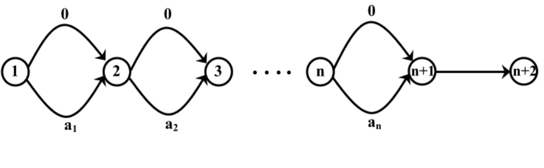
Proof. Given a number partition problem, we will transform it into a minimum excess time walk problem on the network shown in Figure 1. We construct the network G = (N, A) with node set N = {1, 1', 2, 2', ... , n+1, (n+1)', n+2}. For each i = 1 to n, we introduce an arc from i to i+1 with d_i,i+1(t) = a_i for each value of t. Moreover, we also introduce arcs (i, i') and (i', i+1) each with a travel time of 0 independent of t. Finally, there is one arc (n+1, n+2) with d_n+1,n+2(t) = 1 for t ≠ b, and d_n+1,n+2(t) = 0 for t = b. Hence,

* n 1,n 2

e _{+ +} = 1. Notice that only one arc (n+1, n+2) has time-dependent travel time; all other arcs have fixed travel times. We observe that this network can be represented by O(n) quintuples using interval encodings; hence Q = O(n).

We claim that the number partition problem has a feasible solution if and only if there is a walk in G from node 1 to node n+2 with no excess time. First assume that there is a feasible solution x for the number partition problem. Let W be a walk from node 1 to node n+2 defined as follows: if xi = 1, then W

contains an arc (i, i+1) with travel time ai; if xi = 0, then W contains arcs (i, i') and (i', i+1), each with a

travel time of 0. The walk W also contains the arc (n+1, n+2). Observe that W takes b time units to arrive at node n+1, and then arrives at node n+2 with no excess time. This establishes the first part of the claim. Conversely, let W be a path from 1 to n+2 with no excess time. Then W must include a sub-walk W′ from node 1 to node n+1 that takes b units of time. Let xi = 1 if there is an arc (i, i+1) in W′ with travel time ai,

and let x_i = 0 otherwise. Then, x is a feasible solution to the number partition problem. This establishes the second part of the claim, and completes the proof of the theorem. ♦

We can make the following observations from the proof of the above theorem:

Observation 1: The minimum excess time walk problem is NP-hard even if we restrict e* = 1 or only one

arc (i, j) is allowed to have eij > 0.

Observation 2: The network we construct to transform the number partition problem into the minimum

excess time walk problem is a FIFO network. This implies that the minimum excess time walk problem in a FIFO network is also NP-hard.

Observation 3: The number partition problem is not a strongly NP-hard problem. We shall show in

Section 4 that the excess time walk problem is solvable in pseudo-polynomial time, and is thus also not strongly NP-hard.

Observation 4: The minimum excess time walk problem is a special case of the minimum cost walk

problem. Hence the minimum cost walk problem is also NP-hard. We strengthen this result in Section 3.

3. Complexity of the Minimum Cost Walk Problem

In the previous section, we established that the minimum cost walk problem is NP-hard if α = 0 and β > 0 in which case the problem is the minimum excess time walk problem. This problem remains NP-hard even if e* = 1. In the case when α > 0, we can write the arc costs as cij(t) = d + *ij β/αeij(t).

Observe that if β = 0, the problem reduces to the ordinary shortest path problem. In the case that β = α, the problem can be solved as a shortest path problem if the network is FIFO, as stated earlier. We will show that the minimum cost walk problem is NP-hard for every other choice of α and β.

Theorem 2. Suppose that the cost in the minimum cost walk problem is c_ij(t) = _{d + ij}* _{β/αeij(t). Then the}

minimum cost walk problem is NP-hard for all strictly positive integer values of α and β with α≠β.

Proof. We will carry out a transformation from the number partition problem. Let a1, ..., an, b be input

for the number partition problem. We first consider the case that α > β. Let us assume that each aj is an

integer multiple of α−β and that b is also an integer multiple of α - β. (If not, we would just multiply all integers in the number partition problem by α−β.) We construct a network G = (N, A) with node set N = {1, 1', 2, 2', ... , n+1, (n+1)', n+2}. For each i = 1 to n, we introduce an arc from i to i+1 with d_i,i+1(t) =

* i,i 1

d ₊ = βai/(α-β) for all t. Moreover, we also introduce arcs (i, i') and (i', i+1). The arc (i', i+1) has a

travel time of 0 for all t. For the arc (i, i'), * i,i'

d = 0, and e_i,i'(t) = αa_i/(α-β). (We can ensure that * i,i'

d = 0 by letting di,i'(t) = 0 for some very large value of t.) Note that the cost of arc (i, i+1) is βai/(α-β), and the

cost of arc (i, i') is β/α [αai/(α-β)] = βai/(α-β). Thus the cost of travel from i to i+1 is the same for the two

subpaths from i to i+1. However, the travel times of the two subpaths are different. Note that the difference in travel times of these two subpaths is d_i,i'(t)-d _i,i+1(t) = αa_i/(α-β) - βa_i/(α-β) = a_i. We now consider the arc (n+1, n+2). Let t' = b +

∑

n_i=1βa α β_i/( - ). The arc (n+1, n+2) has *

n 1,n 2

d _{+ +} = 0 and en+1,n+2(t) = 1 for all t and en+1,n+2(t') = 0.

We now claim that there is a path from node 1 to node n+2 with cost

∑

n_i=1βa α β_i/( - ) if and only if there is a solution to the number partition problem. First, assume that there is a feasible solution x for the

number partition problem. Let W be a walk from node 1 to node n+2 defined as follows: if x_i = 1, then W contains the arcs (i, i') and (i', i+1); if xi = 0, then W contains arc (i, i+1). The walk W also contains the

arc (n+1, n+2). Observe that W takes t' time units to arrive at node n+1 and then arrives at node n+2 with no excess time. This establishes the first part of the claim.

Conversely, let W be a path from 1 to n+2 with cost

∑

n_i=1βa α β_i/( - ). Since every path from node 1 to node n+1 has cost

∑

_i=1n βa α β_i/( - ), it follows that the excess time of arc (n+1,n+2) is 0, and so the walk W arrives at node n+1 at time t'. Let x_i = 1 if there is an arc (i, i') in W′, and let x_i = 0 if there is an arc (i, i+1) in W. Then, x is a feasible solution to the number partition problem. This establishes the second part of the claim.

We have proved the result in the case that α > β. The case that α < β is similar. In this case, we would let _d*_{i,i 1+ = βai/(β-α) and ei,i'(t) = αai/(β-α) with other terms being defined the same as above for}

arcs (i, i+1), (i, i') and (i', i+1) for i = 1 to n. In this case, the cost of each arc (i, i+1) and (i, i') is βa_i/(α-β), and arc (i, i+1) has a travel time that is ai greater than the travel time of arc (i, i'). The remainder of the

proof is analogous to the case that α > β. ♦

4. A Pseudo-Polynomial Time Algorithm for the Minimum Cost Walk Problem

In this section, we once again consider the case in which α > 0 and β > 0, and α ≠ β. If we view both α and β as fixed, the algorithm that we develop to solve the minimum cost walk problem runs in time that is polynomial in n, m, and e*. In the case that e* itself is polynomial in n and m, this algorithm is polynomial regardless of the magnitudes of the actual travel times.

Working with the Time Expanded Network

A standard approach for dealing with dynamic network problems is to construct a time-expanded network. We denote the time-expanded network by GT. For a given network G = (N, A), the network GT = (NT, AT) is as follows. For each node i ∈ N, there are T+1 copies i₀, i₁, i₂, ..., i_T in NT, where node i_k represents node i in G at time k. For each arc (i, j) ∈ A, there are multiple arcs (at most T) corresponding to different starting times. There is an arc (i_k, j_l) in the time-expanded network whenever (i, j) ∈ A, l - k = dij(k), and l ≤ T. The arc (ik, jl) in the time-expanded network represents traveling along arc (i, j) starting

from node i at time k and arriving at node j at time l = k + dij(k). We set the cost of arc (ik, jl) in the

time-expanded network equal to α_{d +} *_{ij β(dij(k) - d ). By assumption, d}*_{ij ij(k) - d ≥ 0 for each (i, j) and every} *_ij

k, and G has no directed cycles whose travel time is 0. This implies that GT is an acyclic network. The following property is a direct outcome of the construction of GT.

Property 1. For each walk in G starting at time 0 from node i to node j with travel time l ≤ T, there is a path in GT from node i₀ to node j_l. Moreover, the walk and path have the same cost. Similarly, for each path in GT from node i₀ to node j_l, there is a walk in G starting at time 0 from node i to node j with travel time l, and these walks have the same cost.

It is well known that the shortest path problem (that is, determining minimum cost path from node s to every other node) in an acyclic network can be solved in time linear in the number of arcs in the

network (see, for example, Ahuja, Magnanti and Orlin [1]). Since GT _{has O(mT) arcs and is acyclic, we}

can solve the shortest path problem in it in O(mT) time. In this section, we will develop an algorithm that runs faster than O(mT) time when e* grows more slowly than T.

Working with Reduced Travel Times

Suppose that we solve the shortest path problem in G with respect to the travel times _{d . Let P(k)} *_ij

denote the shortest path from node s to node k and π(k) denote its travel time. It follows from the shortest path optimality conditions (see, for example, Ahuja, Magnanti and Orlin [1]) that

π(j) ≤ π(i) + _{d for each arc (i, j) ∈ A, and} *_{ij (2a)}

π(j) = π(i) + _{d for each arc (i, j) ∈ P(k) and each node k ∈ N\{s}.} *_{ij (2b)}

Since arc lengths are nonnegative, we can assume without any loss of generality that π(s) = 0. We define the reduced minimum travel time, d*ijπ , with respect to π as follows: d*ijπ = d + *ij π(i) - π(j). It

follows from (2a) that d*_ijπ ≥ 0 for each arc (i, j) ∈ A, and d*_ijπ = 0 for each arc (i, j) ∈ P(k) and each node k ∈ N\{s}. Let d (t)πij = dij(t) + π(i) - π(j) denote the reduced travel time of arc (i, j). Note that this

transformation does not affect e_ij(t) because e_ij(t) = d_ij(t) - _{d =} *_{ij d (t)}π_{ij - d}*_ijπ _{. Accordingly,c (t)}π_{ij =}

αd*ijπ + βeij(t) denotes the reduced cost of arc (i, j) at time t. The following lemma shows that solving the

minimum cost walk problem with respect to c is equivalent to solving it with respect to the reduced costs cπ.

Lemma 1. A walk W in G from node s to node k is a minimum cost walk with respect to the costs c_ij(t) if and only if it is a minimum cost walk with respect to the reduced costs c (t)ijπ .

Proof. Consider a walk W starting at node s and terminating at node k in G. Then, c(W) - cπ(W) = α(d*(W) - d∗π_{(W)) = α} *

ij (i,j) W∈ d

∑

− α(

_∑

_{(i, j) W∈} (d + (i)- (j))*_ij π π = −α(π(s) - π(k)) = απ(k),

which is a constant for each node k. Therefore, a minimum cost walk from node s to node k with respect to the arc costs c will also be a minimum cost walk from node s to node k with respect to the arc costs cπ.♦ Lemma 2. Let p =β(n-1)e*/min(α, β). Then, every minimum cost walk from node s to any other node k will have reduced travel time no more than  p.

Proof. Recall that P(k) denotes the shortest path from node s to node k with _{d as travel times. We will} *_ij

henceforth refer to P(k) as P. The reduced cost of the path P is

where the second equality follows from (2b) and the last inequality follows from the fact that P has at most n-1 arcs, and each arc has an excess time of at most e*. We will now show that any walk P' with reduced travel time at least p will have reduced cost greater than or equal to cπ(P), and therefore will not be better than the path P. We will prove this result for two cases: α ≥ β and α < β.

Suppose first that α ≥ β. In this case, p = β(n-1)e*/min(α, β) = (n-1)e*. Any walk P' with reduced travel time at least p has a reduced cost at least αp ≥ βp. Since p = (n-1)e*, then the walk P' has a reduced cost of at least β(n-1)e* ≥ cπ_{(P) (from (3)). Next consider the case when α < β. In this case, p =}

β(n-1)e*/min(α,β) = β(n-1)e*/α. Any walk P' with reduced travel time at least p has a reduced cost of at least αp. Since p = β(n-1)e*/α, the reduced cost of the walk P' is at least β(n-1)e* ≥ cπ_{(P) (from (3)). So, in}

both cases, the reduced cost of P = P(k) is less than or equal to the reduced cost of any walk P' with reduced travel time at least β(n-1)e*/min(α, β). Since every reduced travel time is integral, this proves

the theorem. ♦

The Minimum Dynamic Cost Path Algorithm

We are now in a position to describe our algorithm for the minimum cost walk problem.

Step 1. Compute the shortest paths from node s to all other nodes using travel times d*. Let π(j) denote the minimum travel time from node s to node j.

Step 2. Compute the reduced travel times d*ijπ(t) as well as the reduced costs c (t)πij . Construct the

time-expanded network Gp _{with p = β(n-1)e*/min(α, β) in a manner as described earlier but using}

reduced travel times d (t)π_ij instead of the travel times d_ij(t), and using the cost of arc (ik, jl) in the

time-expanded network Gp _{equal to αd}*_ijπ _{+ β(dij(t) - dij). Find the minimum cost path from node}

sto every other node in Gp_.

Observe that Gp is acyclic. This observation follows from the facts that if W is a directed cycle, then dπ(W) =

∑

_(i,j)∈W (d_ij(t) – π(i) + π(j)) =

∑

(i,j)∈W dij(t) ≥ 1 (since there are no zero-time cycles and all

travel times are non-negative). Since Gp has O(np) nodes and O(mp) arcs, we can determine the minimum cost path from node s to all other nodes in O(mp) = O(β(n-1)me*/min(α, β)) time. Hence the

following theorem.

Theorem 3. The minimum cost walk problem in a network G = (N, A) with integer travel times, where d_ij(t) ≥ 0 for all (i, j) and for all t and where there is no zero-time directed cycle, can be solved in O(β(n-1)me*/min(α, β)) time.

For fixed positive values of α and β, the minimum dynamic cost path algorithm allows us to solve the dynamic shortest path problem in O(nme*) time, which can be arbitrarily faster than the standard O(mT) algorithm. Consider, for example, the network shown in Figure 2 where we wish to determine the shortest path from node s to node t. Every path from s to t has exactly K2 _{arcs. If we}

transform the problem by adding nme* to each arc travel time for each t, then the running time of the ninimum dynamic cost path algorithm remains at O(nme*) time. However, the time of the path from s to t increases by K2_{nme* time, and so the O(mT) algorithm runs in O(K}2_nm2_{e*) time. Though the example}

shown in Figure 2 is artificially constructed, it illustrates an important time: whereas the running time of the standard approach depends upon the travel times, the running time of our algorithm depends upon the difference between the maximum and minimum travel times of arcs. We note that, in practice, the

improvement in running time may not be such a large factor; however, an improvement by even a small constant (e.g., 3) can be of practical value.

5. Shortest Routes in Networks with Traffic Lights

The research in this paper was motivated by the following application. Suppose that we want to go from an origin node s to a destination node t in a (road) network G = (N, A) with n = |N| and m = |A|. We assume that G is a directed network where a two-way street is represented by two arcs representing movement in both directions. We assume (as is typical for any road network) that the number of arcs incident on any node are bounded by a constant number. For example, if there is a four-road junction with two-way traffic on each road, then there will be eight arcs incident on the node representing this junction. Thus, we assume that m = O(n). Let d(a, t) denote the travel time on an arc a starting at time t. For notational convenience in this section, we refer to it as arc a instead of (i, j). We assume that d(a, t) satisfies the FIFO property for every arc a.

At some intersections in the road network, there are traffic lights. For simplicity, we assume that each traffic light alternates between red and green lights in a specified fixed pattern. Our approach, however, can be easily extended to the case when traffic light pattern changes with time. As a person travels in this network, travel times depend upon two things: d(a, t) the time needed to traverse arc a, and the waiting time due to the red light before we start traversing the arc. This problem has been studied by

Ahuja et al. [2] in the past; in this paper we give a different algorithm to solve this problem. We also prove new complexity results about this problem.

We study the following three problems:

Minimum Time Route Problem: From node s to every other node in the network, determine a walk with the minimum travel time in the network.

Minimum Excess Time Route Problem: From node s to every other node in the network, determine a walk with the minimum waiting time.

Minimum Cost Route Problem: From node s to every other node in the network, determine a walk with the least cost, which is a linear function of the travel time and the waiting time.

The difference in these problems versus the problems treated in the previous section is that any waiting time at a traffic light is treated as the excess time, but this waiting is not associated with an arc. We will show in this section that the minimum time route problem can be transformed to the minimum time walk problem in an appropriately defined network and hence can be solved very efficiently. We will also show that the minimum cost route problem can be transformed to the minimum cost walk problem and hence can be solved in pseudo-polynomial time using the algorithm described in Section 4.

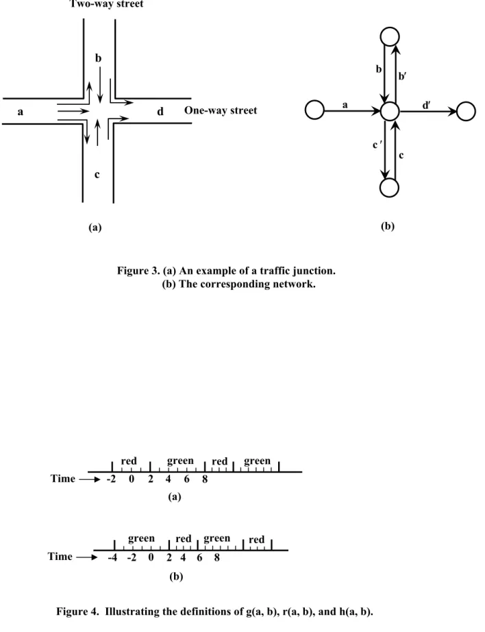
We show in Figure 3(a) an example of a traffic junction created by the intersection of a one-way street with a two-way street. Figure 3(b) shows the corresponding graph at this node. We say that a pair of arcs a and b define a turn if the head node of arc a is the same as the tail node of arc b; we denote this turn

as <a, b>. We say that a turn is a valid turn if one can legally take that turn. For example, the situation

depicted in Figure 3(a) permits the following seven valid turns: <a, b>, <a, c>, <a, d>, <b, c>, <b, d>, <c, b> and <c, d>. We assume that each valid turn has a repetitive pattern of green and red lights phases. We specify this sequence for each turn by defining three values for each valid turn:

g(a, b): the duration of the green phase; r(a, b): the duration of the red phase; and

h(a, b): the smallest amount of time on or before time 0 when the green phase begins.

The value (r(a, b) + g(a, b)) denotes the cycle time, the time after which the light pattern repeats

itself. The value h(a, b) allows us to identify for what time intervals lights will be red and green. We illustrate h(a, b) it using the two examples shown in Figure 4. For the situation depicted in Figure 4(a), h(a, b) = 8, and for the situation shown in Figure 4(b), h(a, b) = 4. For both the situations, g(a, b) = 6, and r(a, b) = 4.

Now suppose that we know the triplet {g(a, b), r(a, b), h(a, b)} for each valid turn <a, b>. Also suppose that we arrive at the head node of the arc a at time t and we need to turn into arc b. We want to determine how long we need to wait before there is a green light. The waiting time for any turn <a, b> is a function of both a and b and when we are ready to take the turn. We will now derive the expression for the waiting time w(a, b, t) which denotes the time we need to wait at turn <a, b> starting at time t (when we are ready to take the turn). Let t = t mod(r(a, b) + g(a, b)). Observe that the green or red phase at time

t will be the same as at time t.

Now suppose that h(a, b) = 0. In this case, the green phase begins at time 0 and the waiting time in this case will be given by the following expression:

0 if t g(a, b),

w(a,b, t) =

r(a,b) g(a, b) t otherwise. < 



+ −

 (4)

Next consider the case when h(a, b) > 0. In this case, the green phase starts at time –h(a, b). Let t = (t + h(a, b)) mod(r(a, b) + g(a, b)). Then t gives the time elapsed since the latest green phase before time t and using (4) we can determine the waiting time for the turn.

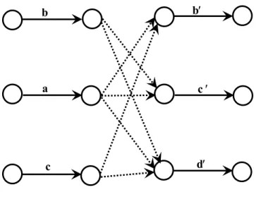
In order to capture the effects of traffic lights through the model described in Section 4, we will transform the graph G into a graph G′ = (N′, A′). Our transformation is similar to that for the shortest paths with turn penalties (see, for example, Ahuja, Magnanti and Orlin [1], pp. 130). Shortest paths with turn penalties arise in traffic networks where taking different turns have different associated penalties. An example of this could be the crossing where a left turn is harder than the right turn (or, vice-versa, in left-driving countries). For the graph in Figure 3(a), we show this transformation in Figure 5. In the transformed network, we take a node with k incident arcs and "split" it into k nodes so that each incoming arc ends at a separate node and each outgoing arc emanates from a separate node. For each valid turn <a, b>, we create a “connection” arc (a, b) in the transformed network connecting the inbound arc a to the outbound arc b. Hence, the network G′ has two types of arcs – arcs that are also in G, which we refer to as regular arcs, and connection arcs that are not in G. Observe that at each junction node, there are as

many connection arcs as the number of turns allowed at the traffic junction. This transformation increases the size of the network. However, since the number of arcs in a traffic network incident to a node is a constant number (typically, no more than 8), the number of arcs and nodes are multiplied by a constant number to obtain G′. Consequently, n′ = |N′| = O(n) and m′ = |A′| = O(n).

In the transformed network G′, we set the travel time of a regular arc a at time t equal to d(a, t). We set the travel time of a connection arc (a, b) at time t equal to w(a, b, t). (Note that the minimum times for these arcs are 0, and so w(a, b, t) is viewed as excess time, as we stated earlier.) There is one-to-one correspondence between paths in G and G′ and they have the same travel times. By assumption, regular arcs in A′ satisfy the FIFO property and it follows from (4) that the connection arcs too satisfy the FIFO property. Hence the graph G′ satisfies the FIFO property, and we can solve the shortest path problem in it

in O(m + n log n) time = O(n log n) time (Kirbi and Potts [9], Kaufmann and Smith [8], and Pallottino and Scutella [12]). We summarize our discussion with the following theorem.

Theorem 4. The minimum time route problem in a traffic network can be solved in O(n log n) time.

Let w* be the maximum cycle time for a light, that is w* = max{r(a, b) + g(a, b): <a, b> is a valid

turn}. Then w* is an upper bound on the excess time at all connection arcs. As before, e* is an upper

bound on the excess time at all regular arcs. We can use the results of Section 4, and obtain the following theorem.

Theorem 5. If α, β > 0, then the minimum cost route problem in a traffic network can be solved in O(β(n-1)m max{e*, w*}/min{α,β}) time.

It follows from Observation 1 that the minimum cost route problem is NP-hard problem even if there is a traffic light at just one junction. We will strengthen this result to show that the minimum cost route problem is NP-hard even if e* = 0, and w* is bounded by a polynomial in n. In other words, the NP-hardness for the traffic light problem can be derived from the effects of traffic lights rather than the effects of different travel times on regular arcs, and does not rely on long cycle times.

Theorem 6. The problem of minimizing waiting times at traffic lights is NP-hard even if restricted to problems in which e* = 0 and w*≤ n2.

Proof. We will carry out a transformation as in Theorem 1 from the number partition problem. The number partition problem remains NP-hard even if we restrict attention to instances in which b ≤ 2n_{. Let}

q1, q2, ..., qk denote the prime numbers that are less than n2. By the prime number theorem, k is

approximately n2_{/(ln n}2_{) > n}3/2_{. Therefore,} k

i 1=

∏

q_i > 2n _{> b.}

We first create nodes 1 to n+1 as in the transformation used in the proof of Theorem 1. We also create nodes n+2, ..., n+k+1 such that the travel time (ignoring lights) to get from node n+j to n+j+1 is 0 for each j = 1 to k. We also create a sequence of k traffic lights, one on each of n+1, ..., n+k such that the time between the start of two successive green phases at the light at node n+j is q_j. This light is green for exactly one time unit per phase followed by a red interval of q_j - 1 time units. Finally, the initial green interval is chosen so that each light is green at time b. Let φ_j ≡ b(mod q_j) for j = 1 to k.

By construction, if one arrives at time b at traffic node n+1, then one can travel from node n+1 to node n+k+1 in 0 time units, since each traffic light will be green and all travel times are 0. Moreover, if one arrives at node n+1 at any time t < 2n _{such that t ≠ b, then at least one of the traffic lights on nodes}

n+1, ..., n+k will be red. To see this, note that if all lights are green at time t, then t ≡ φ_j (mod q_j) for all j. But since

∏

_{i 1}k₌ q_i > 2n_{, there is at most one value of t satisfying these k congruences such that t < 2}n_{. So,}

it must be the case that t = b.

Since nodes 1 to n+1 have the same construction as in the proof of Theorem 1, there is a solution to the number partition problem if and only if there is a path from node 1 to node n+1 of travel time b. This occurs if and only if there is a path from node 1 to node n+k+1 with no waiting time at traffic lights.

Acknowledgements

We thank the referees for their insightful comments and suggestions which led to an improved presentation of results. The first author gratefully acknowledges the support of NSF Grant DMI-9900087. The research of the second author was supported by the NSF Grant DMI-9820998 and the Office of Naval Research Grant ONR N00014-98-1-0317.

References

[1] R.K.Ahuja, T.L. Magnanti and J.B. Orlin, Network flows: Theory, Algorithms, and Applications,

Prentice Hall, Englewood Cliffs, NJ, 1993.

[2] R.K.Ahuja, J. B. Orlin, S. Pallottino, and M. G. Scutellà, Minimum time and minimum cost path problems in street networks with periodic traffic lights, to appear in Transportation Science

2002.

[3] I. Chabini, A new shortest path algorithm for discrete dynamic networks, Proceedings of the 8th

IFAC Symposium on Transport Systems, Chania, Greece, June 16-17 (1997), 551-556.

[4] I. Chabini, Discrete dynamic shortest path problems in transportation applications: Complexity and algorithms with optimal run time, Transportation Research Record 1645 (1998), 170-175.

[5] I. Chabini, Fastest paths in dynamic networks, to appear in Transportation Science 2002.

[6] S.E. Dreyfus, An appraisal of some shortest-path algorithms, Operations Research 17(1969),

395-412.

[7] M.L. Fredman, and R.E. Tarjan, Fibonacci heaps and their uses in improved network optimization algorithms, Journal of ACM 34 (1987), 596-615.

[8] D.E. Kaufmann, and R.L. Smith, Fastest paths in time-dependent networks for intelligent vehicle-highway systems application, IVHS Journal 1 (1993), 1-11.

[9] R.F. Kirby, and R.B. Potts, The minimum route problem for networks with turn penalties and prohibitions, Transportation Research 3 (1969), 397-408.

[10] A. Orda, and R. Rom, Shortest-path and minimum-delay algorithms in networks with time-dependent edge length, Journal of the ACM 37 (1990), 607-625.

[11] A. Orda, and R. Rom, Minimum weight paths in time-dependent networks, Networks 21 (1991),

295-320.

[12] S. Pallottino, and M.G. Scutellà, Shortest path algorithms in transportation models: Classical and innovative aspects, Equilibrium and Advanced Transportation Modelling, P. Marcotte and S.

Nguyen (Eds.), Kluwer Academic Publishers, pp. 245-281, 1998.

[13] W.W. Wardell, and A. K. Ziliaskopoulos, A intermodal optimum path algorithm for dynamic multimodal networks, European Journal of Operational Research 125 (2000), 486-502.

[14] A.K. Ziliaskopoulos, Optimum path algorithms on multidimensional networks: Analysis, design, implementation and computational experience, Ph.D. Dissertation, University of Texas at Austin, 1994.

[15] A.K. Ziliaskopoulos, and H.S. Mahmassani, On finding least time paths considering delays for intersection movements, Transportation Research 30B (1996), 359-367.

Figure 1. Transforming a number partition problem into a minimum excess time walk problem. 11 21 31 K-11 K1 12 ₂2 ₃2 _K-12 _K2 13 ₂3 ₃3 _K-13 _K3 1K 2K 3K K-1K KK 1 2 3

….

n n+1 n+2 0 0 0 a1 a2 an

a

b

c

d

One-way street Two-way street

Figure 3. (a) An example of a traffic junction. (b) The corresponding network.

a d′ b b′ c c ′ (a) (b)

red green red green 0 2 4 6 8 (a) red red green green -4 -2 0 2 (b) -2 4 6 8 Time Time

a

b b′

c

c ′

d′

Figure 5. Transforming the minimum time route problem into a minimum time walk problem.