HAL Id: hal-00299119
https://hal.archives-ouvertes.fr/hal-00299119
Submitted on 16 Apr 2004
HAL is a multi-disciplinary open access
archive for the deposit and dissemination of
sci-entific research documents, whether they are
pub-lished or not. The documents may come from
teaching and research institutions in France or
abroad, or from public or private research centers.
L’archive ouverte pluridisciplinaire HAL, est
destinée au dépôt et à la diffusion de documents
scientifiques de niveau recherche, publiés ou non,
émanant des établissements d’enseignement et de
recherche français ou étrangers, des laboratoires
publics ou privés.
Aspects of risk assessment in power-law distributed
natural hazards
S. Hergarten
To cite this version:
S. Hergarten. Aspects of risk assessment in power-law distributed natural hazards. Natural Hazards
and Earth System Science, Copernicus Publications on behalf of the European Geosciences Union,
2004, 4 (2), pp.309-313. �hal-00299119�
SRef-ID: 1684-9981/nhess/2004-4-309
© European Geosciences Union 2004
and Earth
System Sciences
Aspects of risk assessment in power-law distributed natural hazards
S. Hergarten
Institute of Geology, University of Bonn, Germany
Received: 7 October 2003 – Revised: 25 February 2004 – Accepted: 3 March 2004 – Published: 16 April 2004 Part of Special Issue “Multidisciplinary approaches in natural hazards”
Abstract. Risk assessment is mainly based on certain
sce-narios involving an event of a certain size which is thought to be characteristic for the considered type of hazard. However, many natural hazards extend over a wide range of event sizes, and some of them are even free of characteristic scales. An expression for the risk taking into account various event sizes is derived, and its implications on risk assessment for earth-quakes, forest fires, landslides, and rockfalls are discussed. Under simple assumptions on the damage as a function of the event size, it turns out that the total risk is governed by either the small number of large events or the majority of small events. The distinction between these two classes de-pends on both the power-law exponent of the event size dis-tribution and the damage function. For earthquakes, forest fires, and rockfalls, the total risk is mainly constituted by the largest events, while results are non-unique for landslides.
1 From hazard to risk assessment
Risk assessment is a straightforward extension of hazard as-sessment towards economic sciences. While hazard assess-ment concerns the probability of occurrence of a certain event, risk assessment takes into account its effects on life, civilization, and economics, too.
Although the term risk has several meanings in everyday life, there is a more or less unique definition of risk in the context of natural and man-made hazards. Let N be the ex-pected (mean) number of events of a certain type in a cer-tain region and time interval. Determining this number, per-haps including its spatial and temporal variation and its de-pendence on environmental conditions, is the main goal of hazard assessment. Let further D be the expected damage caused by an event of the considered type. The risk R is then defined by
R = N D. (1)
Correspondence to: S. Hergarten
According to this definition, the risk R is the expected dam-age caused by events of a certain type within a certain region and time interval.
Although this definition is straightforward, it suffers from the restriction to events of a certain type. This restriction does not only concern the class of phenomena under consid-eration, e.g. earthquakes, landslides, rockfalls, storms or for-est fires, but also the magnitude of the event. Thus, we cannot use Eq. (1), e.g. to determine the risk of earthquakes at San Francisco, but only to determine the risk of earthquakes of a certain magnitude there.
In those cases where a typical event size can be assigned to the considered phenomenon, this restriction is no prob-lem. However, event sizes vary strongly for most natural hazards, such as earthquakes, landslides, rockfalls or forest fires. In the example of earthquakes, an increase in mag-nitude by one unit (e.g. from magmag-nitude 6 to magmag-nitude 7) corresponds to an increase in released energy by a factor of about 30. Thus, an earthquake of magnitude 8 releases about 1000 times more energy than an earthquake of magnitude 6. Both are able to cause considerable damage, and the question is whether a few events of magnitude 8 cause more damage than the rather large number of magnitude 6 earthquakes or not.
The same applies to many other natural hazards, such as landslides, rockfalls, and forest fires. The largest histori-cal rockfall in the Alps involved a rock volume of more than 9 km3, while other rockfalls are only a few cubic me-ters large. A single forest fire may destroy several thousand square kilometers of forest, while the majority of forest fires is much smaller.
As a result of the large range of event sizes in many nat-ural hazards, Eq. (1) must be replaced with an expression that regards all possible event sizes, their frequency of occur-rence, and the damage corresponding to the event size. Let P (s)be the cumulative size distribution of the considered phenomenon, i.e. the probability that the size of an arbitrary event is greater than or equal to s. In this context, s may be any measure of event size, e.g. magnitude, released energy
310 S. Hergarten: Aspects of risk assessment in power-law distributed natural hazards or size of the rupture area in case of earthquakes, affected
area or displaced volume in case of landslides and rockfalls or destroyed area in case of forest fires.
In order to evaluate the risk regarding events of different sizes, we first need the expected damage of one event with respect to the size distribution P (s). Let p(s) be the corre-sponding probability density according to
p(s) = −dP (s)
ds , (2)
and D(s) the expected damage induced by an event of size s. As a result of basic statistics, the expected damage is D =
Z
p(s) D(s) ds, (3)
where the integration extends over all possible event sizes. From this, the total risk is immediately obtained to
R = N D = N Z
p(s) D(s) ds. (4)
Thus, risk assessment regarding event sizes involves two steps:
1. Determining the total number of events in a certain re-gion, time span, and environment, N , and the size distri-bution of the events, P (s). The result is often expressed directly in terms of the product of both, which is called the frequency-magnitude relation.
2. Assessing the damage of an event as a function of its size.
The first step is the goal of hazard assessment, which has taken a major place in research on natural hazards in the last decades. Size distributions of some natural hazards are re-viewed in the following section. In contrast, the second step is the transition from hazard to risk. It may be much more complicated than hazard assessment. There may be cases such as small forest fires or landslides where the damage to be expected can be directly computed, but as soon as events become large enough to affect the socio-economic network including loss of life, reliable estimates may become diffi-cult. For this reason, risk assessment is mainly restricted to single scenarios, such as an earthquake of a given magnitude, while in general a large number of scenarios covering a wide range of event sizes is required. So it seems to be necessary to introduce assumptions on the dependence of the damage on the event size, D(s). Simple assumptions and their impli-cations are discussed in Sects. 3–6.
2 Power-law distributions in natural hazards
Most natural hazards do not only cover a wide range of event sizes, but also exhibit scale-invariant (also called frac-tal) statistics. Earthquakes are the most prominent example, although their fractal character may be hidden behind the logarithmic definition of earthquake magnitudes. As men-tioned above, an increase of magnitude by one unit roughly
corresponds to an increase in released energy by a factor 30. Therefore, the relation for the number N (m) of earthquakes per unit time interval with a magnitude greater than or equal to m found by Gutenberg and Richter (1954),
log10N (m) = A − Bm, (5)
can be transformed into a statistical distribution of the re-leased energies E:
N (E) ∼ E−2B3 (6)
where N (E) is the number of earthquakes per unit time inter-val with an energy release greater than or equal to E. The the-ory behind this transformation was introduced by Kanamori and Anderson (1975); brief reviews are given in almost all textbooks on seismology (e.g. Lay and Wallace, 1995; Aki and Richards, 2002) and in some books on fractals in earth sciences (e.g. Turcotte, 1997; Hergarten, 2002).
If we switch to a more general notation and denote ar-bitrary measures of event size by s, earthquakes follow a power-law size distribution
P (s) ∼ s−b. (7)
If earthquake sizes are measured in terms of released en-ergy, the power-law exponent is b=2B/3. The parameter B slightly varies from region to region, but is generally be-tween about 0.8 and 1.2 (Frohlich and Davis, 1993), so that bfalls into the range between about 0.5 and 0.8.
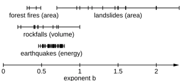
Power-law distributions were found in some other natural hazards, too. For landslides, a rather strong variation in the exponent b was found, but this variation could be neither at-tributed to the triggering mechanism (e.g. rainfall, snow melt or earthquakes), climate, type of landslide nor to the geolog-ical setting. A review was given, e.g. by Hergarten (2003); the values of the exponent b listed there are given in Fig. 1. It was concluded that most of the studies resulted in values of bbetween 1.0 and 1.6 if landslide size is measured in terms of affected area. However, the range may in fact be narrower because there is still some uncertainty about the effect of the method used for data analysis.
Rockfalls are a type of gravity-driven mass movements which strongly differs from most other types (e.g. slides in the strict sense or flows). Their size distributions have been addressed in several studies, too. Results are reviewed and discussed by Dussauge et al. (2002, 2003). Power-law dis-tributions were mainly found with respect to the volume of displaced rock. Similar to landslides, a strong variation in the exponents was observed (from about 0.2 to 1.0), but part of this variation may be artificial as a result of different methods of analysis. As shown in Fig. 1, most of the values fall into the range between 0.4 and 0.7. However, these values are not directly comparable to those of landslides listed above since the former refer to areas, while the latter refer to volumes. It is mostly assumed that the volume of the displaced rock increases with the area to the power of 3/2, so that the size distribution of rockfalls should be a power law with respect
to the area, too. As a result of this transformation, the ex-ponents increase by a factor 3/2, so that range of exex-ponents mentioned above turns into a range from 0.6 to about 1.0 with respect to areas. So the power-law exponents of rock-falls seem to be smaller than those of landslides; the conse-quences of this difference will be discussed later.
Forest fires are another example of power-law distributed natural hazards. Since the fractal properties of forest fires were recently discovered (Malamud et al., 1998), available statistics are smaller than for earthquakes and landslides. There is still a considerable uncertainty about the validity of power-law distributions in forest-fire statistics and concern-ing the exponents b of the distributions. The range of expo-nents reported so far is 0.31≤b≤0.49 if the burnt area is the measure of event size.
3 Event size and damage
In some cases, the damage D(s) may be a linear function of the event size s. This may be the case, e.g. for forest fires as long as they are not too large. Damage may then simply be determined by the amount of destroyed wood which is proportional to the burnt area. However, there are several aspects which make the damage function more complicated in general:
– For some natural hazards, such as earthquakes, events
below a certain size do not cause any damage, so that D(s)is zero there.
– In return, there may an event size leading to total
de-struction, so that D(s) is constant above this event size.
– In the range between these sizes, D(s) will
proba-bly grow stronger than linearly with the event size. This may result directly from properties of the process (e.g. because large landslides are more likely to achieve high velocities than small landslides), but also from the event’s increasing consequences on economy and hu-man life.
– The damage function may even be discontinuous, e.g.
loss of life may introduce steps in D(s). In some cases, these steps may be rather large, e.g. if a nuclear power plant is affected by an earthquake.
4 A simple damage model
Since estimating the damage function requires detailed knowledge on the process and on the goods and human be-ings exposed to danger, we now switch to one of the simplest models of damage, a power-law dependence
D(s) = α sβ. (8)
As mentioned above, β may be one in some cases, but will mostly be larger. However, there may be even situations
0 0.5 1 1.5 2
exponent b forest fires (area)
earthquakes (energy) rockfalls (volume)
landslides (area)
Fig. 1. Power-law exponents of the cumulative size distributions
of some natural hazards. The tickmarks refer to the four forest-fire data sets analyzed by Malamud et al. (1998), the studies on land-slides compiled by Hergarten (2003), the rockfall data analyzed and reviewed by Dussauge et al. (2002, 2003), and 38 earthquake cat-alogs from various geographic regions (Frohlich and Davis, 1993, Table 1, last column).
where β is smaller than unity, which means that the damage increases weaker than linearly with the event size. Imagine an important road crossing a forest, and that a certain eco-nomic damage occurs if this road cannot be used because the forest close to the road is burning. Let us, for simplicity, as-sume that forest-fire areas are circular shaped, and that fires occur at random locations. Under these assumptions, a fire of radius r causes damage if its center is located in a strip of width 2r (r each left and right of the road) around the road. Therefore, the probability that a randomly located fire causes damage increases linearly with the radius r, and thus with the square root of the area, so that β=0.5 in this case.
5 The role of the minimum and maximum event sizes
Before evaluating the risk formula (Eq. (4)), we must spec-ify the power-law distribution (Eq. (7)) more precisely. It is well-known that a power-law distribution can only hold over a limited range of scales in reality, so that cutoff effects at large as well as at small event sizes occur. A discussion of cutoff effects in power-law distributions is given, e.g. by Her-garten (2002). In the simplest cutoff model, only events with sizes between a minimum size sminand a maximum size smax occur. The corresponding probability density function is p(s) = b
smin−b −s−bmax
s−b−1 (9)
(e.g. Hergarten, 2002). From this, we immediately obtain the total risk to R = N Z smax smin b smin−b −smax−b s−b−1α sβds = N bα β − b smaxβ−b−sminβ−b smin−b −smax−b . (10)
As long as the power-law distribution extends over some or-ders of magnitude, we can assume that smaxis much larger
312 S. Hergarten: Aspects of risk assessment in power-law distributed natural hazards than smin. In this case, the behavior of Eq. (10) strongly
de-pends on the difference β − b.
If β > b, the term smaxβ−bis much larger than sβ−bmin, so that
R ≈ N bα β − b
smaxβ−b smin−b −s−bmax
= N
β − bsmaxp(smax) D(smax). (11) Thus, the total risk is mainly determined by the largest events.
In the opposite case, β<b, the increase of the damage with event size is not sufficient to compensate the decrease in fre-quency of event occurrence. The term smaxβ−bbecomes much smaller than sminβ−b, so that the total risk is
R ≈ N bα b − β
sminβ−b smin−b −s−bmax
= N
b − β sminp(smin) D(smin). (12) In this case, the risk mainly arises from the large number of small events, while large events are less important.
Equation (10) is only valid if β6=b. In the special case β = b, the integral in Eq. (10) is computed to
R = N bα smin−b −smax−b logsmax smin =s p(s) D(s)logsmax smin (13) for any arbitrary value of s between sminand smax. Thus, the risk can neither be expressed in terms of smaxalone, nor in terms of sminalone. Both small and large events contribute to the total risk in this case.
The case β=b looks like a theoretical case which is hardly achieved in reality. However, if the difference between smax and sminis only a few orders of magnitude and β comes close to b, both small and large events contribute to the total risk. As an example, we assume that the power law distribution extends over three orders of magnitude, i.e. smax=1000 smin and that β−b=0.1. Then, smaxβ−b≈2 sminβ−bin Eq. (10), so that the risk is clearly not dominated by the large events alone. So there is a region between both regimes where large and small events contribute to the total risk.
6 Implications for earthquakes, forest fires, rockfalls, and landslides
As discussed in Sect. 2, the exponent b of the earthquake size distribution is in the range between 0.5 and 0.8 if event size is measured in terms of released energy. Although quantifying the damage caused by earthquakes of different sizes is dif-ficult, it can be expected that the damage increases stronger than linearly with the released energy, so that the exponent β exceeds 1. Thus, the difference β−b is always positive, and
the total risk resulting from earthquakes is dominated by the largest events.
It is noteworthy that the largest event is not the largest his-torically recorded event. It is the largest event that is possible or better, smaxis the event size where the power law distri-bution breaks down. Especially in regions with a moderate seismic activity, this size may be much larger than the maxi-mum size obtained from historical earthquake catalogs. De-tailed information on geology, especially on the size of the largest faults in a region, is necessary in order to assess the maximum event size.
Things are similar in case of forest fires. The exponent b with respect to the area is rather small (between about 0.3 and 0.5), which means that large events play an important part in forest-fire statistics. As a result, the difference β−b will be greater than 0.5 if damage is proportional to the burnt area, and will remain positive even in the case where the ques-tion is whether roads are blocked by the fire (β=0.5). Thus, the total risk related to forest fires will be determined by the largest events. However, assessing the size of the largest events may be even more difficult than for earthquakes where much research on this topic has been done. None of the forest-fire data analyzed by Malamud et al. (1998) reveals a clear upper cutoff of the power-law; instead, statistics be-come small at large sizes. So the question is whether the power-law distribution may hold up to the sizes of the largest forested areas or whether there is a cutoff at some smaller size. The lack of information on the maximum event size may be a severe problem in risk assessment with respect to forest fires.
As mentioned above, the power-law exponents b of land-slides and rockfalls apparently differ. With respect to areas, a range from 0.6 to 1.0 was given for rockfalls, and a range from 1.0 to 1.6 for landslides. If we assume the simplest damage model, i.e. that the damage is proportional to the af-fected area (β=1), we obtain β−b ∈ [0.0, 0.4] for rockfalls and β−b ∈ [−0.6, 0.0] for landslides. So the difference in the exponents seems to be critical for risk assessment. In the simple, linear damage model, the total risk of rockfalls arises from the largest events, while the large number of small events makes the major contribution in the example of landslides.
However, it should be mentioned the these results are less unique than the results for earthquakes and forest fires. Firstly, the difference β−b approaches zero at the borders of the ranges of b given above. Secondly, the result strongly de-pends on the assumptions on the damage model. If we, e.g. switch to the model where damage occurs if a road is blocked (β=0.5), a large part of the rockfall data sets falls into the range where risk is dominated by the small events. However, this may be unrealistic because small rockfall deposits are not very likely to block a road and can easily be removed. So rockfalls in fact seem to belong to the class of natural hazards where risk is dominated by large events. In return, assuming a damage model where the damage increases stronger than linearly with the event size (β>1), which is not unrealistic, probably brings landslides into this class, too.
7 Conclusions
Many natural hazards extend over several orders of mag-nitude in event size, and some of them even exhibit scale-invariant properties over a considerable range of scales. Assessing risk with regard to this phenomenon requires the determination of damage as a function of the event size, which may be difficult. However, some general results can be obtained from a simple, power-law damage model. It turns out that the overall risk is governed by either the largest or the smallest events. For earthquakes, forest fires, and rockfalls, the largest events are dominant. The results for landslides are non-unique; it depends on the assumptions of the damage model whether the largest or the smallest events are more important for the total risk.
Acknowledgement. The author would like to thank B. D. Malamud and F. Guzzetti for their helpful comments and suggestions. Edited by: T. Glade
Reviewed by: one referee
References
Aki, K. and Richards, P. G.: Quantitative Seismology, University Science Books, Sausalito, California, 2nd edn., 2002.
Dussauge, C., Grasso, J.-R., and Helmstetter, A.: Statistical ana-lysis of rockfall volume distributions: Implications for rockfall dynamics, J. Geophys. Res., 108, 2286, 2003.
Dussauge, C., Helmstetter, A., Grasso, J.-R., Hantz, D., Desvar-reux, P., Jeannin, M., and Giraud, A.: Probabilistic approach to rock fall hazard assessment: potential of historical data analysis, Natural Hazards and Earth System Sciences, 2, 15–26, 2002. Frohlich, C. and Davis, S. C.: Teleseismic b values; or, much ado
about 1.0, J. Geophys. Res., 98, 631–644, 1993.
Gutenberg, B. and Richter, C. F.: Seismicity of the Earth and Asso-ciated Phenomenon, Princeton University Press, Princeton, 2nd edn., 1954.
Hergarten, S.: Self-Organized Criticality in Earth Systems, Springer, Berlin, Heidelberg, New York, 2002.
Hergarten, S.: Landslides, sandpiles, and self-organized criticality, Natural Hazards and Earth System Sciences, 3, 505–514, 2003. Kanamori, H. and Anderson, D. L.: Theoretical basis of some
em-pirical relations in seismology, Bull. Seismol. Soc. Am., 65, 1072–1096, 1975.
Lay, T. and Wallace, T. C.: Modern Global Seismology, Interna-tional Geophysics Series, vol. 58 of Academic Press, San Diego, 1995.
Malamud, B. D., Morein, G., and Turcotte, D. L.: Forest fires: an example of self-organized critical behavior, Science, 281, 1840– 1842, 1998.
Turcotte, D. L.: Fractals and Chaos in Geology and Geophysics, Cambridge University Press, Cambridge, New York, Melbourne, 2nd edn., 1997.