Sharing a resource with randomly arriving foragers

HAL Id: hal-01294950

https://hal.inria.fr/hal-01294950

Submitted on 31 Mar 2016

HAL is a multi-disciplinary open access

archive for the deposit and dissemination of

sci-entific research documents, whether they are

pub-lished or not. The documents may come from

teaching and research institutions in France or

abroad, or from public or private research centers.

L’archive ouverte pluridisciplinaire HAL, est

destinée au dépôt et à la diffusion de documents

scientifiques de niveau recherche, publiés ou non,

émanant des établissements d’enseignement et de

recherche français ou étrangers, des laboratoires

publics ou privés.

Sharing a resource with randomly arriving foragers

Pierre Bernhard, Frédéric Hamelin

To cite this version:

Pierre Bernhard, Frédéric Hamelin. Sharing a resource with randomly arriving foragers. Mathematical

Biosciences, Elsevier, 2016, 273 (91), pp.91-101. �10.1016/j.mbs.2016.01.004�. �hal-01294950�

Contents lists available atScienceDirect

Mathematical Biosciences

journal homepage:www.elsevier.com/locate/mbs

Sharing a resource with randomly arriving foragers

Pierre Bernhard

a,∗

_{, Frédéric Hamelin}

b

a_{BIOCORE team, INRIA-Sophia Antipolis Méditerranée, B.P. 93, F-06902 Sophia Antipolis Cedex, France} b_{AGROCAMPUS OUEST, UMR 1349 IGEPP, F-35042 Rennes Cedex, France}

a r t i c l e

i n f o

Article history:

Received 4 May 2015 Revised 25 November 2015 Accepted 11 January 2016 Available online 19 January 2016 Keywords: Foraging Functional response Random population Poisson process

a b s t r a c t

We consider a problem of foraging where identical foragers, or predators, arrive as a stochastic Poisson process on the same patch of resource. We provide effective formulas for the expected resource intake of any of the agents, as a function of its rank, given their common functional response. We give a gen-eral theory, both in finite and infinite horizon, and show two examples of applications to harvesting a common under different assumptions about the resource dynamics and the functional response, and an example of application on a model that fits, among others, a problem of evolution of fungal plant parasites.

© 2016 Elsevier Inc. All rights reserved.

1. Introduction

The theory of foraging and predation has generally started with the investigation of the behavior of a lone forager[3,15]or of an infinite population of identical foragers, investigating the effect of direct competition [18,19,28] or their spatial distribution[7,16,17]. Then, authors investigated fixed finite groups of foragers in the concept of “group foraging”[4,8,9].

This article belongs to a fourth family where one considers for-agers arriving as a random process. Therefore, there are a finite number of them at each time instant, but this number is varying with time (increasing), and a priori unbounded. We use a Pois-son process as a model of random arrivals. PoisPois-son processes have been commonly used in ecology as a model of encounters, either of a resource by individual foragers, or of other individuals[1,26]. However, our emphasis is on foragers (or predators) arriving on a given resource. There do not seem to be many examples of such setups in the existing literature. Some can be found, e.g. in [10– 12], and also[29](mainly devoted to wireless communications, but with motivations also in ecology).

In[11], the authors consider the effect of the possibility of ar-rival of a single other player at a random time on the optimal diet selection of a forager. In [10,12], the authors consider an a priori unbounded series of arrivals of identical foragers, focusing on the patch leaving strategy. In these articles, the intake rate as a function of the number of foragers —or functional response— is

∗ _{Corresponding author.}

E-mail addresses:Pierre.Bernhard@inria.fr(P. Bernhard), fhamelin@agrocampus-ouest.fr(F. Hamelin).

within a given family, depending on the density of resource left on the patch and on the number of foragers (and, in[12]on a scalar parameter summarizing the level of interference between the for-agers). And because the focus is on patch leaving strategies, one only has to compare the current intake rate with an expected rate in the environment, averaged over the equiprobable ranks of ar-rival on future patches.

In the current article, we also consider an a priori unbounded series of random arrivals of identical foragers, but we focus on the expected harvest of each forager, as a function of its rank and ar-rival time. Our aim is to give practical means of computing them, either through closed formulas or through efficient numerical algo-rithms. These expressions may later be used in foraging theory, e.g. in the investigation of patch leaving strategies or of joining strate-gies[25].

In Section 2, we first propose a rather general theory where the intake rate is an arbitrary function of the state of the system. All foragers being considered identical, this state is completely de-scribed by the past sequence of arrivals and current time.

In Section 3, we offer three particular cases with specific re-source depletion rates and functional responses, all in the case of “scramble competition” (see[10]). But there is no a priori obstruc-tion to dealing also with interference. The limitaobstruc-tion, as we shall see, is in the complexity of the dynamic equation we can deal with.

We only consider the case of a Poisson process of arrivals, mak-ing the harvestmak-ing process of any player a Piecewise Determin-istic Markov Process (PDMP). Such processes have been investi-gated in the engineering literature, since[27]and[24]at least. As far as we know, the term PDMP (and even PDMDP for Piecewise http://dx.doi.org/10.1016/j.mbs.2016.01.004

Deterministic Markov Decision Process, but we have no decision here) was first introduced in[5]. Their control, the decision part, was further investigated, in e.g.[6,31]and a wealth of literature. Later articles such as[2,13]have concentrated on asymptotic prop-erties of their optimal trajectories, and applications in manufactur-ing systems.

These articles (except[5]who proposes general tools for PDMP parallel to those available for diffusion processes) focus on ex-istence and characterization of optimal control strategies. When they give means of calculating the resulting expected payoff, it is through a large (here infinite) set of coupled Hamilton–Jacobi (hy-perbolic) partial differential equations. Here, we want to focus our attention on the problem of evaluating this payoff when the intake rates, the equivalent of strategy profiles of the control and games literature, for each number of players present on the common, are given; typically a known functional response. We take advantage of the very simple structure of the underlying jump process (dis-cussed below), and of the continuous dynamics we have, to obtain closed form, or at least numerically efficient, expressions for the expected payoff, which we call Value for brevity.

2. General theory

2.1. Notation

Data: t1, T,

λ

,

{

Lm

(

·, ·

)

, m∈ N

}

.

Result sought Vn(·), n ∈ N.

t1∈ R Beginning of the first forager’s activity.

T∈ (t1,∞] Time horizon, either finite or infinite.

t∈ [t1, T] Current time.

m

(

t

)

∈ N Number of foragers present at time t.

tm Arrival time of the mth forager. (A Poisson

pro-cess.)

τ

m Sequence

(

t2, t3, . . . tm

)

of past arrival times.

Tm

(

t

)

⊂ Rm−1 Set of consistent

τ

m(t): {(

τ

m

|

t1< t2!!! < tm≤ t}.

λ

∈ R+ Intensity of the Poisson process of arrivals.

δ

∈ R+ Actualization factor (intensity of the random

death process).

Lm

(

τ

m, t

)

∈ R+ Intake rate of all foragers when they are m on the

common.

Mm

(

t

)

∈ R+ Sum of all possible Lm(t), for all possible

τ

m∈

Tm

(

t

)

.

Jm(

τ

m) Reward of forager with arrival rank m, given the

sequence

τ

mof past arrival times. (A random

vari-able.)

V1∈ R+ First forager’s expected reward.

Vm

(

τ

m

)

∈ R+ Expected reward of the forager of rank m.

J_m(n)

(

τ

m

)

Reward of player m if the total number of arriving

foragers is bounded by n. (Random variable) Vm(n)

(

τ

m

)

∈ R+ Expectation of Jm(n)

(

τ

m

)

.

2.2. Statement of the problem

We aim to compute the expected harvest of foragers arriving at random, as a Poisson process, on a resource that they somehow have to share with the other foragers, both those already arrived and those that could possibly arrive later. At this stage, we want to let the process of resource depletion and foraging efficiency be arbitrary. We shall specify them in the examples ofSection 3.

2.2.1. Basic notation

We assume that there is a single player at initial time t1. Whether t1 is fixed or random will be discussed shortly. At this stage, we let it be a parameter of the problem considered. Then identical players arrive as a Poisson process of intensity

λ

, player number m arriving at time tm. The state of the system, (if t1 is

fixed) is entirely characterized by the current time t, the current number of foragers arrived m(t), and the past sequence of arrival times that we call

τ

m(t):

∀

m≥ 2 ,

τ

m:=

(

t2, t3, . . . , tm

)

,

a random vector. The intake rate of any forager at time t is there-fore a function Lm(t)(

τ

m(t), t).

Let the horizon be T, finite or infinite. We may just write the payoff of the first player as

J1

(

t1

)

=

! T t1

e−δ(t−t1)_L

m(t)

(

t2, . . . , tm(t), t

)

dt .

(We will often omit the index 1 and the argument t1 of J1 or V1.) We shall also be interested in the payoff of the nth player arrived:

Jn

(

τ

n

)

=

!T tn

e−δ(t−tn)_L

m(t)

(

τ

m(t), t

)

dt .

(We shall often, in such formulas as above, write m for m(t) when no ambiguity results.) The exponential actualization exp

(

−

δ

t

)

will be discussed shortly. We always assume

δ

≥ 0. In the finite horizon problem, it may, at will, be set to

δ

= 0.

2.2.2. Initial time t1

In all our examples, the functions Lm(

τ

m, t) only depend on

time through differences t− t1, or t− tm, tm− tm−1, . . . t2− t1. They are shift invariant. We believe that this will be the case of most applications one would think of. In such cases, the results are in-dependent of t1. Therefore, there is no point in making it random. If, to the contrary, the time of the day, say, or the time of the year, enters into the intake rate, then it makes sense to consider t1 as a random variable. One should then specify its law, may be ex-ponential with the same coefficient

λ

, making it the first event of the Poisson process. In this case, our formulas actually depend on

t1, and the various payoff Vn should be taken as the expectations

of these formulas.

One notationally un-natural way of achieving this is to keep the same formulas as below (in the finite horizon case), let t1= 0, and decide that, for all m ≥ 2, tm is the arrival time of the forager

number m− 1. A more natural way is to shift all indices by one, i.e. keep the same formulas, again with t1= 0, and decide that

τ

m:=

(

t1, t2, . . . , tm

)

, andTm

(

t

)

=

{τ

m

|

0 < t1<· · · < tm≤ t

}

.

2.2.3. Horizon T

The simplicity of the underlying Markov process in our Markov Piecewise Deterministic Process stems from the fact that we do not let foragers leave the resource before T once they have joined. The main reason for that is based upon standard results of foraging theory that predict that all foragers should leave simultaneously, when their common intake rate drops below a given threshold. (See[3,10,12].)

When considering the infinite horizon case, we shall systemat-ically assume that the system is shift invariant, and, for simplicity, let t1= 0. A significant achievement of its investigation is in giv-ing the conditions under which the criterion converges, i.e. how it behaves for a very long horizon. Central in that question is the ex-ponential actualization factor. As is well known, it accounts for the case where the horizon is not actually infinite, but where termi-nation will happen at an unknown time, a random horizon with an exponential law of coefficient

δ

. It has the nice feature to let a bounded revenue stream give a bounded pay-off. Without this discount factor, the integral cost might easily be undefined. In that respect, we just offer the following remark:

Proposition 1. If there exists a sequence of positive numbers {$m}

such that the infinite series

%

m$m converges, and the sequence of

functions {Lm(·)} satisfies a growth condition

then the infinite horizon integral converges even with

δ

= 0. As a matter of fact, we then have

|

J1|≤ !∞ 0

|

Lm(t)

|

dt≤ !∞ 0 $m(t)dt= ∞ " m=1

(

tm+1− tm

)

$m, and hence EJ1≤ 1

λ

∞ " m=1 $m,

ensuring the convergence of the integral. (Notice however that this is not satisfied by the first two examples below, and not an issue for the third.)

2.2.4. Further notation

We will need the following notation:

∀

m≥ 2 , Tm

(

t

)

=

{τ

m∈ Rm−1

|

t1< t2<· · · < tm≤ t

}

,

(a better notation would be Tm

(

t1, t

)

, but we omit t1for simplicity)

and

M1

(

t

)

= L1

(

t

)

,

∀

m≥ 2 , Mm

(

t

)

=

!

Tm(t)

Lm

(

τ

m, t

)

d

τ

m. (1)

More explicitly, we can write, for example

M3

(

t

)

= ! T t1 dt2 !T t2 dt3 ! T t3 L3

(

t2, t3, t

)

dt = ! T t1 dt !t t1 dt3 ! t3 t1 L

(

t2, t3, t

)

dt2.

These Mm(t) are deterministic functions, which will be seen to

suf-ficiently summarize the Lm(

τ

m, t), a huge simplification in terms

of volume of data. The explanation of their appearance is in the fact that once t and m(t) are given, all sequences

τ

m∈ Tm

(

t

)

are

equiprobable. That is why only their sum comes into play. It will be weighted by the probability that that particular m(t) happens.

To give a precise meaning to this notation, we make the fol-lowing assumption, where Tm

(

t

)

stands for the closure of the set

Tm

(

t

)

:

Assumption 1. Let Dm be the domain

{

(

t,

τ

m

)

∈ R × Rm−1

| τ

m∈

Tm

(

t

)

}

.

∀

m∈ N

\{

1

}

, the functions Lm(·, ·) are continuous from Dm

toR.

As a consequence, the fact that Mm be defined as an integral

over a non-closed domain is harmless. For integration purposes, we may take the closure of Tm. This also implies that each of the

Lm( ·, t) is bounded. Concerning the bounds, we give two

defini-tions:

Definition 1.

1. The sequence of functions {Lm} is said to be uniformly bounded

by L if

∃

L > 0 :

_∀

t > t1,

∀

m∈ N ,

∀τ

m∈ Tm

(

t

)

,

|

Lm

(

τ

m, t

)

|

≤ L .

2. The sequence of functions Lmis said to be exponentially bounded

by L if

∃

L > 0 :

_∀

t > t1,

∀

m∈ N ,

∀τ

m∈ Tm

(

t

)

,

|

Lm

(

τ

m, t

)

|

≤ Lm.

Remark 1.

1. If the sequence {Lm} is uniformly bounded by L, it is also

expo-nentially bounded by max {L, 1}.

2. If the sequence is exponentially bounded by L ≤ 1, it is also uniformly bounded by L.

2.3. Computing the Value 2.3.1. Finite horizon

We consider the problem with finite horizon T, and let V1be its value, i.e. the first forager’s expected payoff. We aim to prove the following fact:

Theorem 1. If the sequence {Lm} is exponentially bounded, then, the

Value V1= EJ1 is given by

V1= !T t1 e−(λ+δ)(t−t1) ∞ " m=1

λ

m−1_M m

(

t

)

dt . (2)

Proof. We consider the same game, but where the maximum

number n of players that may arrive is known. In this game, let

Jm(n)

(

τ

m

)

be the payoff of the problem starting at the time tmof

ar-rival of the mth player, and Vm(n)

(

τ

m

)

be its conditional expectation

given

τ

m. We have for m < n:

Jm(n)

(

τ

m

)

=







































!tm+1 tm e−δ(t−tm)_L m

(

τ

m, t

)

dt +e−δ(tm+1−tm)_J(n) m+1

(

τ

m, tm+1

)

if tm+1< T , !T tm e−δ(t−tm)_L m

(

τ

m, t

)

dt if tm< T < tm+1, 0 if tm≥ T . (3) and Vn(n)

(

τ

n

)

= Jn(n)

(

τ

n

)

=

'

!T tn e−δ(t−tn)_L n

(

τ

n, t

)

dt if tn< T , 0 if tn≥ T .

We now perform a calculation analogous to that in[11]. We want to evaluate the conditional expectation of Jm(n), given

τ

m. The

ran-dom variables involved in this expectation are the tkfor k≥ m + 1.

We isolate the variable tm+1, with the exponential law of tm+1− tm.

Because of the formula (3), we must distinguish the case where

tm+1≤ T from the case where tm+1> T, which happens with a probability exp

(

−

λ

(

T− tm

))

. As for the tk with higher indices

k, we use the definition of the expectation given

(

τ

m, tm+1

)

as EJ(n) m+1

(

τ

m, tm+1

)

= Vm(n+1)

(

tm, tm+1

)

. We get Vm(n)

(

τ

m

)

= ! T tm

λ

e−λ(tm+1−tm)

(

!tm+1 tm e−δ(t−tm)_L m

(

τ

m, t

)

dt +e−δ(tm+1−tm)_V(n) m+1

(

τ

m, tm+1

)

)

dtm+1 +e−λ(T−tm) ! T tm e−δ(t−tm)_L m

(

τ

m, t

)

dt .

Using Fubini’s theorem, we get

Vm(n)

(

τ

m

)

= ! T tm

*

!T t

λ

e−λ(tm+1−tm)_dt m+1

+

e−δ(t−tm)_L m

(

τ

m, t

)

dt + ! T tm

λ

e−(λ+δ)(tm+1−tm)_V(n) m+1

(

τ

m, tm+1

)

dtm+1 +e−λ(T−tm) !T tm e−δ(t−tm)_L m

(

tm, t

)

dt.

The inner integral in the first line above integrates explicitly, and its upper bound exactly cancels the last term in the last line. We also change the name of the integration variable of the second line from tm+1 to t. We are left with

Vm(n)

(

τ

m

)

= ! T tm e−(λ+δ)(t−tm)

,

_L m

(

τ

m, t

)

+

λ

Vm(n+1)

(

τ

m, t

)

-dt . (4)

We may now substitute formula(4)for V₂(3)in the same formula for V₁(3): V₁(3)

(

t2, t3

)

= ! T t1 e−(λ+δ)(t2−t1)

*

L1

(

t2

)

+

λ

!T t2 e−(λ+δ)(t3−t2) ×

.

L2

(

t2, t3

)

+

λ

!T t3 L3

(

t2, t3, t

)

dt

/

dt3

+

dt2.

Using again Fubini’s theorem, we get

V₁(3)

(

t2, t3

)

= !T t1 e−(λ+δ)(t−t1)_L 1

(

t

)

dt +

λ

!T t1 e−(λ+δ)(t−t1)

0

! t t1 L2

(

t2, t

)

dt2

1

dt +

λ

2! T t1

*

_{! t} t1

0

_!t t2 e−(λ+δ)(t3−t1)_L 3

(

t1, t2, t3, t

)

dt3

1

dt2

+

dt

We may now extend the same type of calculation to V₁(n). We find V₁(n)= n−1 " m=1

λ

m−1!T t1 e−(λ+δ)(t−t1)_M m

(

t

)

dt+

λ

n−1 × ! T t1 ! Tn(t) e−(λ+δ)(tn−t1)_L n

(

τ

n, t

)

d

τ

ndt, (5)

or, equivalently, let

∀

m < n , Mm(n)= Mm, M(nn)

(

t

)

= ! Tn(t) e(λ+δ)(t−tn)_L n

(

τ

n, t

)

d

τ

n, (6) V₁(n)= n " m=1

λ

m−1! T t1 e−(λ+δ)(t−t1)_M(n) m

(

t

)

d

τ

n.

Now, if the sequence {Lm} is exponentially, respectively uniformly,

bounded by L (seeDefinition (1)), we get

|

Mm

(

t

)

|

≤

(

t− t1

)

m−1

(

m− 1

)

! L m_{, resp}

_|

_M m

(

t

)

|

≤

(

t− t1

)

m−1

(

m− 1

)

! L, (7)

and the last integral over Tn

(

t

)

in Eq. (5)is a fortiori less in

ab-solute value than |Mn(t)|, since Lm is multiplied by a factor less

than 1.

We can now take the limit as n→ ∞. For each finite n, we have a sum Sn. Call S,n the sum without the last term. The sum in(2)is

limn→∞S,n. Because of the remark above Sn− S,n→ 0 as n → ∞.

Hence Sn and S,nhave the same limit as n→ ∞. Moreover, the

es-timation of Mm(t) above implies that the series in Eq.(2)converges

absolutely. Therefore the theorem is proved. !

Corollary 1.

• If the sequence {Lm} is exponentially bounded by L, then

|

V_1|≤ L

λ

(

L− 1

)

−

δ

,

e[λ(L−1)−δ](T−t1)_{− 1}

-

_{, i f}

_λ

₍

_L−1

₎

₋

_δ

_{-= 0,}

|

V1

|

≤

(

T− t1

)

L i f

λ

(

L−1

)

−

δ

=0.

• If the sequence {Lm} is uniformly bounded by L, then

|

V_1|≤L

δ

(

e−

δ(t−t1)_{− 1}

₎

_{i f}

_δ

_{-= 0 ,}

|

V_1|≤ L

(

T− t1

)

, i f

δ

= 0 .

• The above two inequalities become equalities if Lm is constant

equal to L.

It is worth mentioning that this also yields the value Vm(

τ

m)

for the mth player arriving at time tmgiven the whole sequence of

past arrival times

τ

m. We need extra notation:

∀

n≥ m ,

τ

n m=

(

tm+1, . . . , tn

)

,

τ

n=

(

τ

m,

τ

mn

)

, Tmn

(

tm, t

)

=

{τ

mn

|

tm≤ tm+1≤ . . . ≤ tn≤ t

}

, and Mn n

(

τ

n, t

)

= Ln

(

τ

n, t

)

,

∀

n > m , Mmn

(

τ

m, t

)

= ! τn m∈Tmn(tm,t) Ln

(

τ

m,

τ

mn, t

)

d

τ

mn.

Corollary 2. The value of the mth arriving player given the past

se-quence

τ

mof arrival times is

Vm

(

τ

m

)

= !T tm e−(λ+δ)(t−tm) ∞ " k=m

λ

k−m_Mk m

(

τ

m, t

)

dt . 2.3.2. Infinite horizon

We now tackle the problem of estimating the expectation of

J1=

! ∞ 0

e−δt_L

m(t)

(

τ

m, t

)

dt .

(We have in mind a stationary problem, hence the choice of initial time 0). We will prove the following fact:

Theorem 2. If the sequence {Lm} is uniformly bounded, or if it is

ex-ponentially bounded by L, and

δ

>

λ

(

L− 1

)

, then the expectation V1

of J1is given by V1= ! ∞ 0 e−(λ+δ)t ∞ " m=1

λ

m−1_M m

(

t

)

dt . (8)

Remark 2. If the sequence {Lm} is exponentially bounded with L

≤ 1, the condition

δ

>

λ

(

L− 1

)

is automatically satisfied (and it is also uniformly bounded).

Proof. We start from the formula (2), set t1= 0, and denote the value with a superindex (T) to note the finite horizon. This yields

V₁(T)= ! T 0 e−(δ+λ)t"∞ m=1

λ

m−1_Mm

₍

_t

₎

_{dt . (9)}

We only have now to check whether the integral converges as T→ ∞. We use then the bounds(7), which show that

• If the sequence {Lm} is exponentially bounded,

2

2

2

2

2

∞ " m=1

λ

m−1_Mm

₍

_t

₎

2

2

2

2

2

≤ Le λLt_,

• If the sequence {Lm} is uniformly bounded ,

2

2

2

2

2

∞ " m=1

λ

m−1_Mm

₍

_t

₎

2

2

2

2

2

≤ Le λt_.

As a consequence, the integral in formula(9)converges as T→ ∞, always if the {Lm} are uniformly bounded, and if

λ

(

L− 1

)

−

δ

<

0 if they are exponentially bounded. _!

Corollary 3. If the sequence {Lm} is exponentially bounded and

δ

>

λ

(

L− 1

)

, then

|

V_1|≤ L

δ

−

λ

(

L− 1

)

,

if the sequence {Lm} is uniformly bounded and

δ

> 0, then

|

V1

|

≤

L

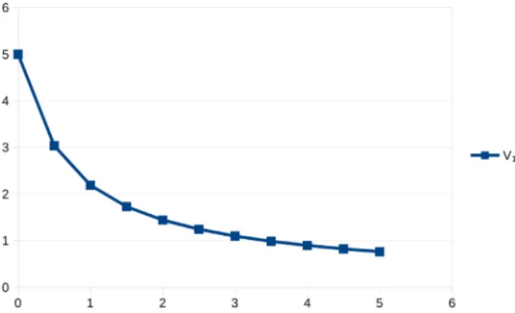
Fig. 1. The decrease of V1asλgoes from 0 to 5 in the simple sharing problem, for

a= 1, T − t1= 5 andδ= 0.

if the Lmare constant and Lm

(

τ

m, t

)

= L, then

V1=

L

δ

.

We also get the corresponding corollary:

Corollary 4. The expected payoff of the mth arriving player given the

past sequence

τ

mof arrival times is:

Vm

(

τ

m

)

= !∞ tm e−(λ+δ)(t−tm) ∞ " k=m

λ

k−m_Mk m

(

τ

m, t

)

dt . (10) 3. Some examples 3.1. Simple sharing 3.1.1. The problem

In this very simple application, we assume that a flux of the desirable good of a units per time unit is available, say a renewable resource that regenerates at the constant rate of a units per time unit, and the foragers present just share it equally. This example may fit biotrophic fungal plant parasites such as cereal rusts (see Appendix B).

3.1.2. The Value

Finite horizon. Thus, in this model (which is not accounted for by

our theory[10]),

∀

t ,

∀

m ,

∀τ

m∈ Tm

(

t

)

, Lm

(

τ

m, t

)

= a

m.

It follows that, in the finite horizon case,

Mm

(

t

)

= a

(

t− t1

)

m−1 m! . Hence, V1= a ! T t1 e−(λ+δ)(t−t1) ∞ " m=1

λ

m−1

₍

_{t− t1}

₎

m−1 m! = a ! T t1 e−(λ+δ)(t−t1)

λ

(

t− t1

)

3

eλ(t−t1)_{− 1}

4

_dt. We immediately conclude:

Theorem 3. For the simple sharing problem in finite horizon, the

value is V1= a ! T−t1 0 e−δt1− e− λt

λ

t dt . (11)

We show in Fig. 1a graph of V1 for a= 1, T = 5 and

δ

= 0 as a function of

λ

, for

λ

∈ [0, 5]. The integral was computed on a spreadsheet by the method of trapezes with a time step of .01.

Infinite horizon. In infinite horizon, we may further use the

identity !∞ 0 e−(λ+δ)t tm−1

(

m− 1

)

!dt= 1

(

λ

+

δ

)

m

easily derived by successive integrations by parts. This immediately yields V1= a ∞ " m=1

λ

m−1 m

(

λ

+

δ

)

m.

We rearrange this expression as

V1= a

λ

∞ " m=1 1 m

0

1 1+δ λ

1

m .

Now, we use the identity, valid for x∈ (0, 1), ∞

"

m=1

xm

m = − ln

(

1− x

)

to obtain the following result:

Theorem 4. For the simple sharing problem in infinite horizon, the

Value is V1= a

λ

ln

0

1+

λ

δ

1

. (12)

One can offer the following remarks:

Remark 3.

• As expected, when

λ

→ 0, V1→ a/

δ

, and V1→ 0 when

λ

→ ∞. • The derivative of V1 with respect to

λ

is always negative,

in-creasing from−a/2

δ

2_for

_λ

_{= 0 to 0 as}

_λ

_{→ ∞.}

• V1is decreasing with

δ

, but diverges to infinity as

δ

→ 0. Finally, we get

Corollary 5. For the simple sharing problem in infinite horizon, the

expected payoff of the mth forager arrived is Vm= a

λ

0

1+

_λ

δ

1

m_{−1 ∞} " k=m 1 k

0

λ

λ

+

δ

1

k = a

λ

0

1+

δ

λ

1

m−1

5

ln

0

1+

λ

δ

1

− m_"−1 k=1 1 k

0

1+

δ

λ

1−k

6

. (13)

A more general formula. At this stage, we have no explicit formula

for the mth arrived forager, m > 1, in finite horizon. We give now two formulas, whose derivations can be found inA.1:

Theorem 5. For the simple sharing problem with horizon T, the

ex-pected reward of the mth arrived forager is given by any of the fol-lowing formulas : Vm(T)

(

tm

)

= a

λ

+

δ

e− (λ+δ)(T−tm) ∞ " $=1

(

λ

+

δ

)

$

₍

_{T− t} m

)

$ $! × $−1 " k=0 1 k+ m

0

1+

_λ

δ

1−k

. (14)

or Vm(T)

(

tm

)

= a

λ

0

1+

δ

λ

1

m−1

5

ln

0

1+

λ

δ

1

− m_"−1 k=1 1 k

0

1+

δ

λ

1−k

6

− a

λ

+

δ

e− (λ+δ)(T−tm) ∞ " k=0 1 k+ m

0

1+

δ

λ

1−k

× k " $=0

(

λ

+

δ

)

$

₍

_{T− t} m

)

$ $! . (15)

The first formula is easier to use for numerical computations, but the second one has the following properties:

Remark 4.

• The second term in the bracket of the first line cancels for m= 1, giving an alternate formula for V1to(11), (but probably less useful numerically),

• the second line goes to 0 as T→ ∞, allowing one to recover formulas(13)and, combining the two remarks(12).

3.2. Harvesting a common: functional response of type 1 3.2.1. Notation

Beyond the notation of the general theory, we have:

x

(

t

)

∈ R+ Available resource at time t.

x1∈ R+ Initial amount of resource in the finite horizon problem.

x0∈ R+ Initial amount of resource in the infinite horizon problem.

a∈ R+ Relative intake rate of all foragers: rate= ax.

b∈ R+ Relative renewal rate of the resource.

c∈ R+ c= b/a: if m > c, the resource goes down.

µ

∈ R+

µ

=

λ

/a a dimensionless measure of

λ

.

δ

∈ R+ Discount factor for the infinite horizon problem.

ν

∈ R+

ν

=

δ

/a. A dimensionless measure of

δ

.

σ

m

σ

m=7mk=1tk. A real random variable.

3.2.2. The problem

We consider a resource x which has a “natural” growth rate b, (which may be taken equal to zero if desired), and decreases as it is harvested by the foragers. Each forager harvests a quantity ax of the resource per time unit. This is a functional response of type 1 in Holling’s classification (see[15]), or “proportional harvesting”, or “fixed effort harvesting”[23]. Assuming that this functional re-sponse does not change with predators density (no interference), we have

∀

t∈

(

tm, tm+1

)

, ˙x =

(

b− ma

)

x , x

(

t1

)

= x1.

3.2.3. Finite horizon

We begin with a finite horizon T and the payoff

J1= !T t1 ax

(

t

)

dt . Define

σ

m= m " k=1 tk. (16)

With respect to the above theory, we have here

Lm

(

τ

m, t

)

= ae(b−ma)(t−tm)e[b−(m−1)a](tm−tm−1)· · · e(b−a)(t2−t1)x1

= aeb(t−t1)_e−a(mt−σm)_x

1.

A more useful representation for our purpose is

Lm

(

τ

m, t

)

= e(b−ma)(t−tm)Lm−1

(

τ

m−1, tm

)

. It follows that Mm

(

t

)

= !t t1 e(b−ma)(t−tm)_M m−1

(

tm

)

dtm, M1

(

t

)

= ae(b−a)(t−t1)x1. (17)

Lemma 1. The solution of the recursion(17)is

Mm

(

t

)

=ae (b−a)(t−t1)

(

m− 1

)

!

0

1− e−a(t−t1) a

1

m−1 x1. (18)

Proof. Notice first that the formula is correct for M1

(

t

)

=

a exp[

(

b− a

)(

t− t1

)

]x1. From Eq. (17), we derive an alternate re-cursion:

d

dtMm+1

(

t

)

= [b −

(

m+ 1

)

a]Mm+1

(

t

)

+ Mm

(

t

)

, Mm+1

(

t1

)

= 0 .

It is a simple matter to check that the formula derived from(18) for Mm+1: Mm+1

(

t

)

= ae(b−a)(t−t1) m!

0

1− e−a(t−t1) a

1

m x1 together with(18)does satisfy that recursion. !

From the above lemma, we derive the following:

Corollary 6. For the proportional foraging game, we have

∞ " m=1

λ

m−1_Mm

₍

_t

₎

_{= a exp}

*

(

b− a

)(

t− t1

)

+

λ

a

(

1− e−a (t−t1)

₎

+

x1.

Substituting this result in(2), we obtain:

Theorem 6. The value of the finite horizon proportional harvesting

problem is as follows: let b a= c ,

λ

a =

µ

, then V1= aeµ !T t1 exp[

(

c−

µ

− 1

)

a

(

t− t1

)

−

µ

e−a(t−t1)] dt x1. or equivalently V1= eµ ∞ " k=0

(

−

µ

)

k k! 1

µ

− c + k + 1

3

1− e−(µ−c+k+1)a(T−t1)

4

_x 1. (19)

Proof. It remains only to derive the alternate, second, formula. It

is obtained by expanding exp[

(

−

µ

exp

(

−a

(

t− t1

))

] into its power series expansion to obtain

V1= aeµ ∞ " k=0

(

−

µ

)

k k! ! T t1 e(c−µ−k−1)a(t−t1)_{d t x} 1

and integrate each term. !

Remark 5. Remark that, although it looks awkward, formula (19) is numerically efficient, as, an alternating exponential-like series, it converges very quickly.

3.2.4. Infinite horizon

It is easy to derive from there the infinite horizon case with the same dynamics, x

(

0

)

= x0, and

J1= a

! ∞ 0

e−δt_x

₍

_t

₎

_{dt .}

Theorem 7. The Value of the infinite horizon proportional

harvest-ing problem is finite if and only if

δ

> b− a −

λ

. In that case it is as follows: let b a= c ,

λ

a =

µ

,

δ

a=

ν

,

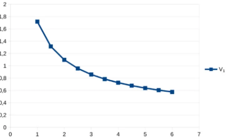
Fig. 2. The decrease of V1asλincreases, here as a function ofµ=λ/a, for the

infinite horizon proportional foraging problem. c= 2,ν= 1, x0= 1.

then V1= aeµ ! ∞ 0 exp[

(

c−

µ

−

ν

− 1

)

at−

µ

e−at] dt x0, or equivalently V1= eµ ∞ " k=0

(

−

µ

)

k k! 1

µ

+

ν

− c + k + 1x0 (20) or equivalently V1= eµ ! 1 0 zµ+ν−c_e−µz_{dz x} 0. (21)

Proof. The first formula above is obtained by carrying the

integra-tion from 0 to∞ instead of from t1 to T. The second formula fol-lows as in the finite horizon case, and the third one, numerically more useful, is obtained by considering the function

F

(

z

)

= eµ ∞ " k=0

(

−

µ

)

k k! zµ+ν−c+k+1

µ

+

ν

− c + k + 1x0, (22)

Clearly, F

(

1

)

= V1. Moreover, the condition of the theorem that

δ

> b− a −

λ

translates into

µ

+

ν

− c + 1 > 0, so that all powers of z in F(z) are positive, and hence F

(

0

)

= 0. Now, differentiate the terms of the series, to obtain

eµzµ+ν−c"∞

k=0

(

−

µ

z

)

k

k! = e

µ_zµ+ν−c_e−µz_.

This is always a convergent series. Hence it represents the deriva-tive F,(z) of F(z). As a consequence, we have

V1= ! 1 0 F,

(

z

)

dz= eµ!1 0 zµ+ν−c_e−µz_{dz x} 0. ! If

µ

+

ν

− c happens to be a positive integer, a very unlikely fact in any real application, successive integrations by parts yield a closed form expression for the integral formula(21).

Remark 6. Clearly, the same remark as in the finite horizon case

holds for formula (20). Formula (21) is even numerically easier to implement. A slight difficulty appears if

µ

+

ν

− c < 0. Remem-ber, though, that it must anyhow be larger than−1. In that case,

F,

(

0

)

= ∞. One may integrate from a small value z0, using the first term of the series(22), F

(

z0

)

. eµzµ0+ν−c+1, as a good approxima-tion of F.

We show inFig. 2a graph of V1 as a function of

µ

, for

µ

∈ [1, 6], for the infinite horizon problem, obtained with formula(21), for

c= 2,

ν

= 1, x0= 1. The integral was computed on a spreadsheet, with the formula of trapezes, with a step size of .01.

3.3. Harvesting a common: functional response of type 2 3.3.1. Notation

Beyond the notation of the general theory, we have:

x∈ R+ Available resource.

x1∈ R+ Initial amount of resource.

a∈ R+ Coefficient of the intake rate.

α

∈ (0, 1) Power parameter of the intake rate = ax1−α_.

p= 1

α−1 Other parametrization of

α

= 1/

(

1+ p

)

.

h∈ R+ _{Duration until exhaustion of the resource if the first} forager remains alone.

q∈ R− Logarithm of the probability that the first forager re-main alone until exhaustion of the resource.

3.3.2. A family of concave functional responses

In this example, we assume a non renewable resource, and foragers or predators with a concave functional response. Specif-ically, if the resource amount is x, the intake rate of a forager is assumed to be ax(1−α)_,

_α

_{∈ (0, 1). This provides us with a}

one-parameter family1 _{of concave functional responses resembling}

Holling’s type 2. By contrast to the laws most commonly used, such as the Michaelis–Menten harmonic law ax/

(

1+ hax

)

[23], and to the curves shown by Holling [15], they lack a plateau at large densities. A distinctive feature is their vertical tangent (infinite derivative) at the origin.2_{It has the nice consequence that it makes}

the resource go to zero in finite time, certainly a more realistic feature than an infinite tail with very low resource left, mainly so if the resource is discrete (number of hosts parasitized, of preys eaten, ...).3_{This makes the problem naturally with a finite horizon,}

and limits to a very small number the probability of having a very large number of foragers participating, although it is not bounded a priori.4

In short, our model is

• less realistic than the harmonic law at high prey densities, • more realistic than the harmonic law at small and vanishing

prey densities. We therefore have:

∀

t∈ [tm, tm+1] , ˙x = −max1−α, x

(

t1

)

= x1. (23) The dynamics(23)immediately integrate into:

_∀

t∈ [tm, tm+1],

xα

₍

_t

₎

₌











xα

₍

_t m

)

−

α

am

(

t− tm

)

if t≤x α

₍

_tm

₎

α

am + tm, 0 if t≥xα

(

tm

)

α

am + tm. (24)

Applying this to the first stage m= 1, we are led to introduce the two parameters

h= x

α

1

α

a and q= −

λ

h (25)

which are respectively the maximum possible duration of the har-vesting activity, assuming a lone forager, and the logarithm of the probability that the first forager be actually left alone during that time. We also introduce two more useful quantities:

p= 1

α

− 1 ,

1_{The parameter a amounts to a simple rescaling of time. The notation x}1−α_was preferred to xα_{because it simplifies later calculations.}

2_{Holling[15]does not give explicit mathematical formulas for the various}

func-tional responses. But we notice that in his Fig. 8, he seems to show a vertical tan-gent at the origin for type 2.

3_{This avoids the paradox of the “atto fox”[20].}

4_{A somewhat unpleasant consequence of this law is that, if the dimension of the}

so that

α

= 1/

(

1+ p

)

, and

∀

r∈ R+,

∀

$∈ N, $ ≥ 2 , Pr

(

1

)

= 1 , Pr

(

$

)

= $−1 8 i=1

(

r+ i

)

. (26) 3.3.3. Expected reward

With these notation we can state the following fact, whose proof is given inA.2.

Theorem 8. For the problem of harvesting a nonrenewable resource

with a functional response L

(

x

)

= axp/(p+1)_{, p a positive real number,}

using q the natural logarithm of the probability that the first forager remains alone until exhaustion of the resource, and notation(26),

Vm+1= xm+1 ∞ " $=1 q$−1 Pp+1

(

$

)

$ " n=1

(

−1

)

$−n

(

$_{− n}

)

! n " k=1 1 k!

(

m+ k

)

n−k. (27)

Remark 7. Several remarks are in order.

• The expected reward of the first forager is therefore obtained by placing m= 0 in the above formula.

• The first term of the power series in q is just 1. Therefore this could be written

V1= x1[1+ qS]

where S is a power series in q. We therefore find that if no other forager may come, i.e.

λ

= 0, hence q = 0, we recover

V1= x1: the lone forager gets all the resource. And since q < 0, V1is less than x1as soon as q-= 0.

• The series converges, and even absolutely. As a matter of fact, it is easy to see that the last two, finite, sums are less than

(

e2₊ 1

)

/2. (Taking the sum of the positive terms only and extending them to infinity.)

• The case p= 1 (i.e.

α

= 1/2) is somewhat simpler. In particular, in that case, Pp

(

$

)

= $!, and Pp+1

(

$

)

=

(

$+ 1

)

!/2.

3.3.4. Numerical computation

We aim to show that, in spite of the unappealing aspect of our formulas, they are indeed very easy to implement numerically. We focus first on the payoff of the first player, i.e. formula(27) with

m= 0.

On the one hand, q being negative, it is an alternating series, converging quickly: the absolute value of the remainder is less than that of the first term neglected, and a fortiori than that of the last term computed. Therefore it is easy to appreciate the pre-cision of a numerical computation. The smaller the intensity

λ

of the Poisson process of arrivals, the faster the series converges. On the other hand, it lends itself to an easy numerical implementation along the following scheme. Let

V1= x1 ∞ " $=1 u$ $ " n=1

v

$−nwn, wn= n " k=1 yn,k. Obviously, u$= q$−1 Pp+1

(

$

)

,

v

n=

(

−1

)

n n! , yn,k= 1 k! kn−k. Therefore, the following recursive scheme is possible :

u1= 1 ,

∀

$ > 1 , u$=

qu$−1

p+ $,

v

0= 1 ,

∀

n > 1 ,

v

n=−

v

n−1

n ,

Fig. 3. The decrease of V1asλincreases from 0 to 5 for the functional response of

type 2, with x1= 1, a = 1,α= .5. y1,1= 1 ,

∀

n > 1 , 1≤ k < n , yn,k= yn−1,k k ,

∀

n > 1 , yn,n= yn−1,n−1 n .

The sequences {un}, {vn} and {wn} need be computed only once.

Altogether, if we want to compute L steps, there are 2L2_{+ 3}

₍

_{L− 1}

₎

arithmetic operations to perform. A small task on a modern com-puter even for L= a few hundreds. Moreover, given the factorials, it seems unlikely that more than a few tens of coefficients be ever necessary, as our limited numerical experiments show. In that re-spect, the computational scheme we have proposed is adapted to the case where |q| is large (

λ

large), lumping the numerator q$−1 with the denominator Pp+1

(

$

)

—which is larger than $!— to avoid multiplying a very large number by a very small one, a numeri-cally ill behaved operation. For small |q| (say, no more than one), one may compute a few coefficients of the power series separately, and then use the polynomial to compute V1for various values of q. We show inFig. 3a plot of V1as a function of

λ

, for

α

= .5, a = 1 and x1= 1. (i.e. a time to exhaustion of the resource for a lone forager equal to two.) It was obtained using the recursive scheme above (in Scilab). For the larger

λ

= 5, we needed 40 terms in the infinite sum (which was also sufficient for

λ

= 6).

Finally, formula (27), giving the expected payoff of an agent arriving when m other agents are present, can clearly be imple-mented numerically along the same scheme as previously, replac-ing yn,k= yn−1,k/k by yn,k= yn−1,k/

(

m+ k

)

.

4. Conclusion

The problem considered here is only that of evaluating the ex-pected reward of these identical agents arriving as a Poisson ran-dom process. This seems to be a prerequisite to many problems in foraging theory in that reasonably realistic framework, although it was avoided in the investigation of the optimal patch leaving strategies[10]. (Notice, however, that our first example is not ac-counted for by that theory.) In that respect, we were able to build a rather general theory, independent of the particular functional response of the foragers and of the resource depletion/renewal mechanism. A nice feature of the theory is that, while the com-plete data of the problem involve the sequence of functions Lm(

τ

m,

t), each a function of m real variables, a very large amount of data,

the result only depends on the sequence of functions of one real variable Mm(t).

Three particular examples, of increasing complexity, all three in scramble competition (no interference), show that this general the-ory can be particularized to more specific contexts, leading to ef-ficient numerical algorithms, if not always to closed formulas. We provide numerical results that do not claim to be representative of any real situation, but are meant to show that the computation can easily be performed, and to display the qualitative aspect of the re-sults. The first two examples: simple, equal, sharing of a constant flux of goods and proportional foraging of a (slowly) renewable re-source, can easily be implemented on a spreadsheet. The example with a functional response of Holling type 2 requires a small pro-gram, that runs essentially instantly. In all three cases, the decrease of V1as

λ

increases look qualitatively similar.

However, we need, as in our examples, to be able to integrate explicitly in closed form the dynamic equation of the resource to compute the Mm sufficiently explicitly. This is why we chose the

particular functional response we proposed as an approximation of a Holling type 2 response. Admittedly a major weakness of this theory so far. What would be needed would be a theory exploit-ing the simple, sequential nature of the Markov process at hand, but not dependent on an explicit integration of the differential dy-namics. An open problem at this stage.

Also, we are far from determining any kind of optimal behavior, such as diet choice as in[11]. But this study was a first necessary step in characterizing the efficiency of the foraging process. Since we have the result for each number of agents present upon join-ing, it may be useful to decide whether an individual should join [25]. Other exciting possibilities for future research include explor-ing further the Simple sharexplor-ing example, which may provide origi-nal insights as to the evolution of the latent period in plant para-sites (Appendix B).

Appendix A. Proofs

A.1. Proof ofTheorem 5

We aim to derive formulas(14)and(15). We shall simplify the notation through the use of

α

:=

λ

+

δ

, and

θ

:= T − tm. We start from Vm= a !T tm e−αθ"∞ k=m

λ

k−m

₍

_{t− tm}

₎

k−m k

(

k− m

)

! dt = a

λ

m ∞ " k=m

λ

k k ! θ 0 e−αt t k−m

(

k− m

)

!dt .

Successive integrations by parts show that

∀

n∈ N , ! θ 0 e−αttn n!= 1

α

n+1

9

1− e−αθ n " $=0

α

$

_θ

$ $!

:

.

Substitute this in the previous formula, to get

Vm= a

α

m−1

λ

m

5

∞ " k=m

λ

k k

α

k− e −αθ"∞ k=m

λ

k k

α

k k_"−m $=0

α

$

_θ

$ $!

6

= a

α

m−1

λ

m

5

∞ " k=m

λ

k k

α

k− e− αθ"∞ $=0

α

$

_θ

$ $! ∞ " k=$+m

λ

k k

α

k

6

.

We use twice the identity

∀

n∈ N , ∞ " k=n

λ

k k

α

k = ln

0

1+

λ

_δ

1

− n−1 " k=1

λ

k k

α

k.

The two terms ln

(

1+

λ

/

δ

)

cancel each other, and we are left with

Vm= a

α

m−1

λ

m

5

− m_"−1 k=1

λ

k k

α

k+ e− αθ"∞ $=0

α

$

_θ

$ $! $+m−1_" k=1

λ

k k

α

k

6

.

We write the last sum over k as a sum from k= 1 to m − 1 plus a sum from k= m to $ + m − 1. The first one cancels with the first sum in the square bracket, to yield

Vm= a

α

m−1

λ

m e− αθ"∞ $=1

α

$

_θ

$ $! $+m−1_" k=m

λ

k h

α

k.

It suffices to re-introduce the leading factor

(

α

/

λ

)

m−1 _{in the last} sum and to shift the summation index k by m to obtain for-mula(14).

To obtain formula(15), interchange the order of summation in the above double sum (all the series involved are absolutely con-vergent): Vm= a

α

m−1

λ

m e−αθ ∞ " k=m

λ

k k

α

k ∞ " $=k−m+1

α

$

_θ

$ $! , and substitute ∞ " $=k−m+1

α

$

_θ

$ $! = e αθ₋ k_"−m $=0

α

$

_θ

$ $! to get Vm= a

α

m−1

λ

m

5

ln

.

1+

α

δ

/

− m_"−1 k=1

λ

k k

α

k− e− αθ"∞ k=m

λ

k k

α

k k−m " $=0

α

$

_θ

$ $!

6

.

Transform the last term in the square bracket as we did to get for-mula(14)to obtain formula(15).

A.2. Proof ofTheorem 8

Expected reward of the first player. We aim to derive formula(27). For simplicity, we start with the expected reward of the first player, i.e. m= 0 in that formula. We remind the reader of nota-tion(25), and we will use the extra notation

b= a1+p

_α

p_{, and}

_σ

m= m " k=1 tk. We remark that bh1+p₌x1

α

=

(

1+ p

)

x1. (A.1)

Now, in formula(24), replace xα_{(tm) by its formula, taken again in}

(24)but for t∈ [tm−1, tm]. To take care of the possibility that zero

be reached, we introduce a notation for the positive part:

[[X]]₊= max

{

X , 0

_}

.

We obtain

xα

(

t

)

= [[xα

₍

_t

m−1

)

−

α

a[

(

m− 1

)(

tm− tm−1

)

+ m

(

t− tm

)

]]]₊.

Iterate this process until expressing xα_{(t) in terms of x}α_(t

1) and finally use notation(16)to obtain

xα

(

t

)

= [[

α

a[h−

(

t2− t1

)

− 2

(

t3− t2

)

− · · ·

−

(

m− 1

)(

tm− tm−1

)

− m

(

t− tm

)

]]]+

=

α

a[[h+

σ

m− mt]]₊.

As a consequence,

Lm

(

τ

m, t

)

= b[[h +

σ

m− mt]]p₊. (A.2)

To keep the formulas readable, we use the notation(26). We are now in a position to state the following fact:

Proposition 2. For Lmgiven by(A.2)with(16), Mmas defined in(1)

is given by M1

(

t

)

= b[[h − t]]₊p, and for m≥ 2:

Mm

(

t

)

= b Pp

(

m

)

m " k=1

(

−1

)

k−1

(

m− k

)

!

(

k− 1

)

![[h− k

(

t− t1

)

]] p+m−1 + . (A.3)

Proof. Observe that the formula is correct for m= 1. Then, we need the simple lemma:

Lemma 2. Let a real number b, two real numbers u < v, and two

positive real numbers $ and r be given. Then

!v u [[b+ $s]]r₊ds= 1 $

(

r+ 1

)

3

[[b+ $

v

]]r₊+1− [[b + $u]]r₊+1

4

.

Proof of the lemma. If b+ $

v

≤ 0, then clearly the integrand is always zero, thus so is the integral, as well as our right hand side (r.h.s.). If b+ $u ≥ 0, the integrand is always positive, as well as the two terms of the r.h.s. This is a simple integration. If u <−$/b <

v

, we should integrate from−$/b to v. Then the lower bound corre-sponds to b+ $s = 0, and we only have the term corresponding to the upper bound, which is what our r.h.s. gives. _!

We use the following representation of Mm:

Mm

(

t

)

= !t t1 dtm !tm t1 dtm−1 !tm−1 t1 dtm−2. . . !t3 t1 [[h+

σ

m− mt]]p₊dt2. To carry out this calculation, we introduce, for m≥ 2 the kernel

Km

(

tm, t

)

= 1 Pp

(

m− 1

)

m_"−1 k=1

(

−1

)

k−1

(

m− k − 1

)

!

(

k− 1

)

! ×[h + kt1+

(

m− k

)

tm− mt]p+m−2, (A.4)

and the quantity

Nm

(

tm+1, t

)

=

! tm+1

t1

Km

(

tm, t

)

dtm.

We first notice that M2 is obtained by taking the positive parts of all terms in bN2(t, t). To get M3(t) we may simply replace ev-erywhere h by h+ t3− t, which behaves as a constant in previous integrations, integrate in t3from t1to t, and take the positive parts of all terms. And so on. It remains to derive the general forms of

Km and Nm by induction. Let us start from the formula given for

Km. Integrating, we get Nm

(

tm+1, t

)

= Pp

(

m

)

−1 m_"−1 k=1

(

−1

)

k−1

(

m−k

)

!

(

k−1

)

! ×[

(

h+kt1+

(

m−k

)

tm+1−mt

)

p+m−1−

(

h+mt1−mt

)

p+m−1]. The second term in the r.h.s. is independent from k. Recognizing combinatorial coefficients, and using

(

1+

(

−1

))

m−1_{= 0, we get}

m−1 " k=1

(

−1

)

k

(

m− k

)

!

(

k− 1

)

! = −1

(

m− 1

)

! m−2 " k=0

(

−1

)

k

0

m− 1 k

1

=

(

−1

)

m−1

(

m− 1

)

!,

which we can include as the term k= m of the sum, leading to

Nm

(

tm+1, t

)

= 1 Pp

(

m

)

m " k=1

(

−1

)

k−1

(

m− k

)

!

(

k− 1

)

! ×[h + kt1−

(

m− k

)

tm+1− mt]m. Taking the positive part of each term in (a2_/2)N

m(t, t) yields

for-mula(A.3), and adding tm+1− t to all terms yields formula analo-gous to(A.4)for Km+1, proving the proposition. !

We therefore have V1 = b ∞ " m=1

λ

m−1 Pp

(

m

)

m " k=1

(

−1

)

k−1

(

m− k

)

!

(

k− 1

)

! × ! h+t1 t1 [[h− k

(

t− t1

)

]]₊p+m−1e−λ(t−t1)dt = b ∞ " m=1

λ

m−1 Pp

(

m

)

m " k=1

(

−1

)

k−1

(

m− k

)

!

(

k− 1

)

! ! h/k 0

(

h− kt

)

p+m−1_e−λt_dt.

Using the power expansion of exp

(

−

λ

t

)

, and then successive inte-grations by parts, we find

!h/k 0

(

h− kt

)

p+m−1e−λtdt= ∞ " $=0 ! h/k 0

(

h− kt

)

p+m−1

(

−

λ

t

)

$ $! dt =

θ

p+m"∞ $=0

(

−

λ

h

)

$ k$+1 m₈+$ i=m

(

p+ i

)

−1_. We substitute this expression in the formula for Mm(t), regroup

powers of

λ

h and products p+ i:

V1= bhp

λ

∞ " m=1 m " k=1

(

−1

)

k+m−1

(

m− k

)

!

(

k− 1

)

! ∞ " $=m

(

−

λ

h

)

$ k$−m+1_Pp

₍

$_{+ 1}

)

.

We take a factor

λ

h out, change the order of summation and use

(A.1)to find V1= x1 ∞ " $=1 q$−1 Pp+1

(

$

)

$ " m=1 m " k=1

(

−1

)

m+k

(

m− k

)

! k! k$−m.

Finally, let n= $ − m + k replace m as a summation index. We ob-tain: V1= x1 ∞ " $=1 q$−1 Pp+1

(

$

)

$ " n=1

(

−1

)

$−n

(

$_{− n}

)

! n " k=1 1 k! kn−k. (A.5)

which is formula(27)with m= 0. !

Expected reward of later players. We focus on the reward of the m+ 1-st arrived player, i.e. when m players are already present. We seek now to instantiate formula(10)with m= n + 1. Let

xm+1= x

(

tm+1

)

,

θ

m+1= xα m+1

α

a and

σ

$ m+1=

σ$

−

σ

m. We easily obtain Lm+n= b

,,

θ

m+1+

σ

mm+1+n− m

(

t− tm+1

)

−

(

m+ n

)

t

--p +. An analysis completely parallel to the previous one leads to

M_mm+n₊₁= _Pb p

(

n

)

n " k=1

(

−1

)

k−1

(

n− k

)

!

(

k− 1

)

![[

θ

m+1−

(

m+ k

)(

t− tm+1

)

]] p+n−1 + .

Using the similarity with formula(A.3), we get formula(27):

Vm+1= xm+1 ∞ " $=1 q$−1 Pp+1

(

$

)

$ " n=1

(

−1

)

$−n

(

$_{− n}

)

! n " k=1 1 k!

(

m+ k

)

n−k. as desired. !

Appendix B. Simple sharing and the evolution of fungal plant parasites

The “Simple sharing” example may fit biotrophic fungal plant parasites such as cereal rusts. These fungi travel as airborne spores. When falling on a plant, a spore may germinate and the fungus may penetrate the plant tissue. Such an infection results in a very small (say 1 mm2_{large) lesion. After a latent period during which} the fungus takes up the products of the plant host’s photosynthe-sis, the lesion starts releasing a new generation of spores.