Comparing sensitivity analysis methods to advance lumped watershed model identification and evaluation

(1)

HAL Id: hal-00298785

https://hal.archives-ouvertes.fr/hal-00298785

Submitted on 1 Nov 2006

HAL is a multi-disciplinary open access

archive for the deposit and dissemination of sci-entific research documents, whether they are pub-lished or not. The documents may come from teaching and research institutions in France or abroad, or from public or private research centers.

L’archive ouverte pluridisciplinaire HAL, est destinée au dépôt et à la diffusion de documents scientifiques de niveau recherche, publiés ou non, émanant des établissements d’enseignement et de recherche français ou étrangers, des laboratoires publics ou privés.

Comparing sensitivity analysis methods to advance

lumped watershed model identification and evaluation

T. Tang, P. Reed, Thibaut Wagener, K. van Werkhoven

To cite this version:

T. Tang, P. Reed, Thibaut Wagener, K. van Werkhoven. Comparing sensitivity analysis methods to advance lumped watershed model identification and evaluation. Hydrology and Earth System Sciences Discussions, European Geosciences Union, 2006, 3 (6), pp.3333-3395. �hal-00298785�

(2)

HESSD

3, 3333–3395, 2006 lumped model sensitivity analysis Y. Tang et al. Title Page Abstract Introduction Conclusions References Tables Figures J I J I Back Close

Full Screen / Esc

Printer-friendly Version

Interactive Discussion

EGU Hydrol. Earth Syst. Sci. Discuss., 3, 3333–3395, 2006

www.hydrol-earth-syst-sci-discuss.net/3/3333/2006/ © Author(s) 2006. This work is licensed

under a Creative Commons License.

Hydrology and Earth System Sciences Discussions

Papers published in Hydrology and Earth System Sciences Discussions are under open-access review for the journal Hydrology and Earth System Sciences

Comparing sensitivity analysis methods

to advance lumped watershed model

identification and evaluation

Y. Tang, P. Reed, T. Wagener, and K. van Werkhoven

Department of Civil and Environmental Engineering, The Pennsylvania State University, University Park, Pennsylvania, USA

Received: 29 September 2006 – Accepted: 27 October 2006 – Published: 1 November 2006 Correspondence to: P. Reed (preed@engr.psu.edu)

(3)

HESSD

Full Screen / Esc

EGU

Abstract

This study tested four sensitivity analysis methods: (1) local analysis using parameter estimation software (PEST), (2) regional sensitivity analysis (RSA), (3) analysis of vari-ance (ANOVA), and (4) Sobol’s method to identify sensitivity tools that will advvari-ance our understanding of lumped hydrologic models for the purposes of model improvement,

5

calibration efficiency and improved measurement schemes. The methods’ relative ef-ficiencies and effectiveness have been analyzed and compared. These four sensitiv-ity methods were applied to the lumped Sacramento soil moisture accounting model (SAC-SMA) coupled with SNOW-17. Results from this study characterize model sensi-tivities for two medium sized watersheds within the Juniata River Basin in Pennsylvania,

10

USA. Comparative results for the 4 sensitivity methods are presented for a 3-year time series with 1 h, 6 h, and 24 h time intervals. The results of this study show that model parameter sensitivities are heavily impacted by the choice of analysis method as well as the model time interval. Differences between the two adjacent watersheds also suggest strong influences of local physical characteristics on the sensitivity methods’

15

results. This study also contributes a comprehensive assessment of the repeatabil-ity, robustness, efficiency, and ease-of-implementation of the four sensitivity methods. Overall ANOVA and Sobol’s method were shown to be superior to RSA and PEST. Relative to one another, ANOVA has reduced computational requirements and Sobol’s method yielded more robust sensitivity rankings.

20

1 Introduction

In this paper we apply and evaluate the differences between four popular sensitivity analysis methods, selected to represent the variety of methods currently used. The four sensitivity analysis methods include: (1) local analysis using the parameter esti-mation software (PEST), (2) regional sensitivity analysis (RSA), (3) analysis of variance

25

(4)

HESSD

Full Screen / Esc

EGU moisture accounting model, a medium complexity spatially lumped rainfall-runoff model

used for river forecasting throughout the USA. The model is implemented in two water-sheds in the Susquehanna River Basin in Pennsylvania and run at hourly, six hourly, and daily time steps.

Broadly, models of watershed hydrology are irreplaceable components of water

re-5

sources studies including flood and drought prediction, water resource assessment, cli-mate and land use change impacts, or non-point source pollution analysis (e.g.,Singh and Woolhiser, 2002). Hydrologic models are evolving from single purpose tools to complex decision support systems that can perform all (or at least many) of the tasks mentioned above in a single software package. In many cases, hydrologists are moving

10

towards models of highly complex environmental systems that include close coupling of surface and groundwater flow processes, feedbacks with the atmosphere, transport of water and solutes, and spatially explicit representations of system characteristics and states (e.g., Duffy, 1996, 2004). In integrated assessment applications models may even include socioeconomic components to integrate human behavior (Wagener

15

et al.,2005). In general, hydrologic models are highly non-linear, contain thresholds, and often have significant parameter interactions. These properties make it difficult to evaluate how models of hydrologic systems behave and which parameters control this behavior during different response modes (e.g.,Demaria et al.,2006). The increasing trend towards more complex models and its potential consequences in terms of

compu-20

tational constraints and obfuscating model impacts on decision making motivates the need for enhanced model identification and evaluation tools (Beven and Freer,2001; Vrugt et al.,2003;Saltelli et al.,2004;Wagener and Kollat,2006).

Hydrologic models play an important role in elucidating the dominant controls on wa-tershed behavior and in this context it is important for hydrologists to identify the

domi-25

nant parameters controlling model behavior. One approach to gain this understanding is through the use of sensitivity analysis, which evaluates the parameter’s impacts on the model response (Hornberger and Spear,1981;Freer et al.,1996;Wagener et al., 2001;Liang and Guo,2003;Hall et al.,2005;Pappenberger et al.,2005;Sieber and

(5)

HESSD

Full Screen / Esc

EGU Uhlenbrook,2005). Sensitivity analysis results can be used to decide which

parame-ters should be the focus of model calibration efforts, or even as an analysis tool to test if the model behaves according to underlying assumptions (e.g.,Wagener et al.,2003). Ultimately, sensitivity methods should serve as diagnostic tools that help to improve mathematical models and potentially help us to identify where gaps in our knowledge

5

are most severe and are most strongly affecting prediction uncertainty. Data gaps are particularly important in the context of guiding field measurement campaigns (Lang-bein, 1979; Moss, 1979; Wagener and Kollat, 2006; Reed et al., 2006). Section 2 provides a more detailed review of existing sensitivity analysis methods and a detailed discussion of the four methods compared in this study.

10

2 Sensitivity analysis tools and sampling schemes

2.1 Overview

Model sensitivity analysis charaterizes the impact that changes in model inputs have on the model outputs in a strict sense. Sensitivity measures are determined mathemat-ically, statistmathemat-ically, or even graphically. There are several prior studies that have broadly

15

reviewed and classified the sensitivity analysis methods that exist (Saltelli et al.,2000, 2004;Helton and Davis,2003;Oakley and O’Hagan,2004;Frey and Patil,2002; Chris-tiaens and Feyen,2002). Any sensitivity analysis approach can be broken up into to two components (Wagener and Kollat, 2006): (1) a strategy for sampling the model parameter space (and/or state variable space), and (2) a numerical or visual measure

20

to quantify the impacts of sampled parameters on the model output of interest. The im-plementation of these two components varies immensely (e.g.,Freer et al.,1996;Frey and Patil,2002;Hamby,1994;Patil and Frey,2004;Pappenberger et al.,2006; Vande-berghe et al.,2006), and guidance is currently lacking to help modelers decide which approach is best suited to the needs of a particular study. Generally, the approaches

25

(6)

HESSD

Full Screen / Esc

EGU et al.,1999;Muleta and Nicklow,2005).

The nominal range and differential analysis methods are two well known local pa-rameter sensitivity analysis methods (Frey and Patil, 2002; Helton and Davis, 2003). Nominal range sensitivity analysis calculates the percentage change of outputs due to the change of model inputs relative to their baseline (nominal) values. The

percent-5

age change is seen as the sensitivity of the corresponding input. Differential analysis utilizes partial derivatives of the model outputs with respect to the perturbations of the model input. The derivative values are themselves the metrics of sensitivity. Further analysis can be conducted by approximating the simulation model using Taylor’s series (Helton and Davis,2003).

10

The nominal range and differential analysis methods have the advantages of being straightforward to implement while maintaining modest computational demands. The major drawback of these methods is their inability to account for parameter interactions, making them prone to underestimating true model sensitivities. Alternatively, global parameter sensitivity analysis methods vary all of a model’s parameters in predefined

15

regions to quantify their importance and potentially the importance of parameter inter-actions.

There are a variety of global sensitivity analysis methods such as regional sensitivity analysis (RSA) (Young,1978;Hornberger and Spear,1981), variance based methods (Saltelli et al., 2000), regression based approaches (Spear et al., 1994; Helton and

20

Davis,2002), and Bayesian sensitivity analysis (Oakley and O’Hagan,2004). Global methods attempt to explore the full parameter space within pre-defined feasible pa-rameter ranges. In this paper, our goal is to test a suite of sensitivity methods and discuss their relative benefits and limitations for advancing lumped watershed model identification and evaluation.

25

The four sensitivity analysis approaches which include PEST, RSA, analysis of vari-ance (ANOVA), and Sobol’s method were selected for comparison due to their popu-larity and large number of applications (Doherty,2003; Doherty and Johnston,2003; Moore and Doherty,2005;Wagener et al.,2003;Lence and Takyi,1992;Freer et al.,

(7)

HESSD

Full Screen / Esc

EGU 1996;Pappenberger et al.,2005;Mokhtari and Frey,2005;Sobol’,1993,2001;Fieberg

and Jenkins,2005;Hall et al.,2005). The sensitivity analysis methods tested in this study range from local to global and capture a broad range of analysis methodologies (differential analysis, RSA, and variance-based analysis). The main characteristics of these four methods are summarized in Table1. In Sect.2.2, each of these approaches

5

and the associated statistical sampling schemes used in this study are discussed in more detail. In the context of this paper we assume that the selection of an appropri-ate numerical measure, is satisfied through two chosen objective functions based on the root mean square error (RMSE) (see5.2). Readers interested in how parameter sensitivity changes with different objective functions can reference the following studies

10

(Wagener et al.,2001;Demaria et al.,2006). 2.2 Sensitivity analysis tools

2.2.1 PEST

PEST, which stands for parameter estimation, is a model independent nonlinear pa-rameter estimation tool (Doherty,2003;Doherty and Johnston,2003;Doherty,2004;

15

Moore and Doherty,2005). PEST was developed to facilitate data interpretation, model calibration and predictive analysis. Like many other parameter estimation or model cal-ibration tools, PEST aims to match the model simulation with an observed set of data by minimizing the weighted sum of squared differences between the two. The opti-mization problem is iteratively solved by linearizing the relationship between a model’s

20

output and its parameters. The linearization is conducted using a Taylor series expan-sion where the partial derivatives of each model output with respect to every parameter must be calculated at every iteration. For each iteration, the solution of the linearized problem is the current optimal set of parameters. The current optimal set is then com-pared to that of the previous time step to determine when to terminate the optimization

25

process. During the linearization step, the forward difference or central difference op-erators can be used for calculating the derivatives. Parameter ranges, initial parameter

(8)

HESSD

Full Screen / Esc

EGU values, and parameter increments must be provided by the user. The parameter vector

is updated at each step using the Gauss-Marquardt-Levenberg algorithm (Marquardt, 1963;Levenberg, 1944). The derivatives of the model outputs with respect to its pa-rameters are calculated and provide a measure of the parameter sensitivities at each iteration. The “composite sensitivity” is provided by PEST as a byproduct of the

pa-5

rameter estimation results. Equation (1) defines the composite sensitivity of parameter

i :

s_i = (JtQJ)1/2_{i i} /m (1)

whereJ is the Jacobean matrix and Q is the cofactor matrix which in most cases is a

diagonal matrix whose elements are composed of squared weights for model outputs.

10

If the model outputs are equally weighted,Q is equal to the identity matrix. The number

of outputs, m, is the number of data records in the time series in this study. Thus s_i is the normalized magnitude of the Jacobean matrix column with respect to parameter i . As expected for a local sensitivity analysis method, Eq. (1) is a univariate analysis of parameter impacts on model outputs (i.e., no parameter interactions are considered).

15

2.2.2 Regional sensitivity analysis using Latin hypercube sampling

RSA (Young,1978;Hornberger and Spear,1981) is also called generalized sensitivity analysis (GSA) (Freer et al.,1996) and has been widely used in hydrology (e.g.Lence and Takyi, 1992; Spear et al., 1994; Freer et al., 1996; Pappenberger et al., 2005; Sieber and Uhlenbrook,2005;Ratto et al.,2006). Monte Carlo sampling and

“behav-20

ioral/nonbehavioral” partitioning are the two major components of this method. Monte Carlo sampling is used to generate n parameter sets in the feasible parameter space defined using a multi-variate uniform distribution. After model evaluations using these parameters, the sets of parameters are decomposed into two separate groups (behav-ioral/good and nonbehavioral/bad) according to the model’s performance or behavior.

25

RSA identifies the difference between the underlying distributions of the behavioral and nonbehavioral groups. Either graphical methods (e.g., marginal cumulative distribution

(9)

HESSD

Full Screen / Esc

EGU function plots) or statistical methods such as Kolmogorov-Smirnov (KS) testing

(Kot-tegoda and Rosso, 1997) are then used to characterize if a parameter significantly impacts behavioral results.

Freer et al.(1996) extended the original RSA by breaking the behavioral parameter sets into ten equally sized groups. (Wagener et al., 2001) modified this approach

5

further by including all parameter sets and avoiding the need to specify behavioral and non-behavioral sets. Instead, the population is divided into ten bins of equal size based on a sorted model performance measure (Wagener and Kollat, 2006). Conclusions about parameter sensitivities are made qualitatively by examining differences in the marginal cumulative distributions of a parameter within each of the ten groups. If the ten

10

lines with respect to ten different groups are clustered, the parameter is not sensitive to a specific model performance measure, i.e., there is no difference in underlying distribution. Conversely, the degree of dispersion of the lines is a visual measure of a model’s sensitivity to an input parameter. Wagener and Kollat (2006) implemented the original idea ofFreer et al.(1996) visually using the Monte Carlo analysis toolbox

15

(MCAT) (Wagener et al.,2001,2003,2004) where the marginal cumulative distributions of the ten groups are plotted as the likelihood value versus the parameter values (e.g., see Figs. 5 and 6).

In this study, Latin hypercube sampling (LHS) was used to sample the feasible pa-rameter space for testing RSA based on the recommendations and findings of prior

20

studies (e.g.Osidele and Beck,2001;Sieber and Uhlenbrook,2005). LHS integrates random sampling and stratified sampling (Mckay et al.,1979;Helton and Davis,2003) to make sure that all portions of the parameter space are considered. The method divides the parameters’ ranges into n disjoint intervals with equal probability 1/n from which one value is sampled randomly in each interval. LHS is generally recommended

25

for sparse sampling of the parameter space and the parameter interactions are ne-glected as noted byWilliam et al.(1999). More details about LHS are available in the following papers (Mckay et al.,1979;Helton and Davis,2003;William et al.,1999).

(10)

HESSD

Full Screen / Esc

EGU 2.2.3 Analysis of variance using iterated fractional factorial design sampling

Assuming model response (e.g., RMSE of streamflow in this study) is normally dis-tributed, the role of ANOVA is to quantify the differences of the mean model responses that result from samples of each parameter. In ANOVA, parameters are “grouped” into particular ranges of parameter values representing intervals with equal

parame-5

ter value width, contrasting to RSA in which parameter sets are “grouped” based on objective values. According to ANOVA terminology, a parameter is called a “factor” and a parameter group is termed a “level” of the factor. ANOVA essentially partitions the model output or response into the overall mean, main factor effects, factor interac-tions, and an error term (Neter et al., 1996;Mokhtari and Frey,2005). Theoretically,

10

ANOVA can capture a range from the first order (main effects from single parameters) to the total order of effects (i.e., all parameter impacts including all interactions). How-ever, it is not feasible to calculate all of the effects for a complex model in practice due to computational limitations. Fortunately, prior studies have shown that second order interactions are usually sufficient for capturing a model’s output variance (Box et al.,

15

1978;Henderson-Sellers et al.,1993;Liang and Guo,2003). Therefore, our analysis focuses on first order and second order effects within the ANOVA model. The ANOVA model with main and second order effects of two factors is shown in Eq. (2):

Y_{i j k} = µ + α_i + β_j + (α × β)_{i j}+ ε_{i j k} (2)

where i and j indicate the levels of factors A and B respectively, α_i is the main effect of

20

i th level of A, β_j is the main effect of jth level of B, (α × β)_{i j} represents the interaction

of A and B. The error term, ε_{i j k}, reflects the effects that are not explained by the main effects and interactions of the two factors.

The F -test is used to evaluate the statistical significance of differences in the mean responses among the levels of each parameter or parameter interaction. The F-values

25

are calculated for all parameters and parameter interactions. The higher the F-values are, the more significant the differences are and therefore the more sensitive the pa-rameter or papa-rameter interaction is. Detailed presentation of the ANOVA calculation

(11)

HESSD

Full Screen / Esc

EGU table for main effects and second order effects can be found in other studies (Neter

et al.,1996;Mokhtari and Frey,2005). In addition to the F-test, the coefficient of de-termination (R2) quantifies how the ANOVA model shown in Eq. (2) captures the total variation of model responses with the inclusion of the second order parameter interac-tions. In cases where parameter interactions are important the coefficient of

determi-5

nation should improve (or increase) with the addition of the interaction term (α × β)_{i j} from Eq. (2).

When applying the ANOVA method the statistical sampling scheme used to quan-tify the model response is a key determinant of the method’s computational feasibility and accuracy. If one parameter or parameter interaction is analyzed at a time in

suc-10

cession, the total number of model runs will be excessively large and most hydrologic applications would be computationally intractable. In this study, the iterated fractional factorial design (IFFD) sampling scheme (Andres and Wayne, 1993; Andres, 1997; Saltelli et al.,1995) was used to limit the computational burden posed by ANOVA while seeking high quality results.

15

IFFD works well when first and second order parameter effects dominate (Andres, 1997). Using IFFD in ANOVA allows users to neglect higher order interactions not included in the model (Liang and Guo, 2003; Andres,1997) while generating highly repeatable results (Saltelli et al.,1995). Consequently, the number of model runs re-quired can be reduced substantially. IFFD as implemented in this study samples the

20

parameters at three different levels: low, middle, and high. The parameter levels are defined as equally spaced intervals within the predefined parameter ranges. Using a small number of factor levels enables the sampling scheme to attain statistically signif-icant results efficiently and accurately (Mokhtari and Frey,2005;Andres,1997). IFFD extends the basic orthogonal fractional factorial design (FFD) by conducting multiple

25

iterations. The basic operations in IFFD include orthogonalization, folding, replication and random sampling (Andres and Wayne,1993;Andres,1997;Saltelli et al.,1995). The orthogonalized design guarantees equal frequency for two parameter combina-tions but also differentiates the main effects from two-way interactions. A detailed

(12)

pre-HESSD

Full Screen / Esc

EGU sentation of IFFD is beyond the scope of this paper. Readers interested in detailed

descriptions of IFFD are referred to the following papers (Andres and Wayne,1993; Andres,1997;Saltelli et al.,1995).

2.2.4 Sobol’s method using quasi-random sequence sampling

In Sobol’s method (Sobol’,1993), the variance of the model output is decomposed into

5

components that result from individual parameters as well as parameter interactions. Conventionally, the direct model output is replaced by a model performance measure such as RMSE as used in this study. The sensitivity of each parameter or parameter interaction is then assessed based on its contribution (measured as a percentage) to the total variance computed using a distribution of model responses. Assuming the

10

parameters are independent, the Sobol’s variance decomposition is shown in Eq. (3):

D(y)=X i D_i +X i <j D_{i j}+ X i <j <k D_{i j k} + D12···m (3)

where D_i is the measure of the sensitivity to model outputy due to the i th component

of the input parameter vector denoted asΘ, D_{i j} is the portion of output variance that results due to the interaction of parameter θ_i and θ_j. The variable m defines the total

15

number of parameters. The variance decomposition shown in Eq. (3) can be used to define the sensitivity indices of different orders shown below in Eq. (4)–(5).

first order S_i = Di D (4) second order S_{i j} = Di j D (5) total S_{T i} = 1 − D∼i D (6) 20

where S_i denotes the sensitivity that results from the main effect of parameter θ_i. The second order sensitivity index, S_{i j}, defines the sensitivity that results from the inter-action of parameters θ_i and θ_j. The average variance, D_∼i, results from all of the

(13)

HESSD

Full Screen / Esc

EGU parameters except for θ_i. The total order sensitivity, S_{T i}, represents the main effect

of θ_i as well as its interactions up to mth order of analysis. A parameter which has a small first order index but large total sensitivity index primarily impacts the model output through parameter interactions.

The variances in Eq. (3) can be evaluated using approximate Monte Carlo numerical

5

integrations. The Monte Carlo approximations for D, D_i, D_{i j}, and D_∼i are given in Eqs. 7-12 as presented in the following prior studies (Sobol’,1993,2001;Hall et al.,2005):

b f₀= 1 n n X s=1 f (Θ_s) (7) b D= 1 n n X s=1 f2(Θ_s) − bf₀2 (8) c D_i = 1 n n X s₌₁

f (Θ(a)_s )f (Θ(b)_{(∼i )s},Θ(a)_{i s}) − bf₀2 (9)

10 c D_{i j}c= 1 n n X s=1

f (Θ(a)_s )f (Θ(b)_{(∼i ,∼j )s},Θ(a)_{(i ,j )s}) − bf₀2 (10) c D_{i j} =Dc_{i j} c −cD_i−cD_j (11) d D_∼i = 1 n n X s₌₁

f (Θ(a)_s )f (Θ(a)_{(∼i )s},Θ(b)_{i s}) − bf₀2 (12) where n is the sample size,Θ_s denotes the sampled individual in the scaled unit hy-percube, and (a) and (b) are two different samples. All of the parameters take their

15

values from sample (a) are represented by Θ(a)_s . The variables Θ(a)_{i s} and Θ(b)_{i s} denote that parameter θ_i uses the sampled values in sample (a) and (b), respectively. The symbolsΘ(b)_{(∼i )s}andΘ(b)_{(∼i )s}represent cases when all of the parameters except for θ_i use the sampled values in sample (a) and (b), respectively. The symbolΘ(a)_{(i ,j )s} represents

(14)

HESSD

Full Screen / Esc

EGU parameters θ_i and θ_j with sampled values in sample (a). Finally, Θ(a)_{(∼i ,∼j )s} represents

the case when all of the parameters except for θ_i and θ_j utilize sampled values from sample (b).

The original Sobol’s method required n×(2m+1) model runs to calculate all the first order and the total order sensitivity indices. An enhancement of the method made

5

by Saltelli (2002) provides the first, second and total order sensitivity indices using

n×(2m+2) model runs. In this study, we implemented this modified version of Sobol’s

methodology to compute the first order, second order and total order indices.

The convergence of the Monte Carlo integrations used in Sobol’s method is heavily affected by the sampling scheme selected. The error term in the Monte Carlo

integra-10

tion decreases as a function of 1/√n given uniform, random samples at n points in the

m-dimensional space. However, in this study we elected to use Sobol’s quasi-random sequence (Sobol’, 1967,1994) to increase the convergence rate to nearly 1/n. The quasi-random sequence samples points more uniformly along the Cartesian grids than uncorrelated random sampling. Details about Sobol’s quasi-random sequence can be

15

found in the following studies (Sobol’,1967,1994;Bratley and Fox,1988;William et al., 1999).

3 Overview of the lumped hydrologic models

The SNOW-17 (Anderson,1973) and the Sacramento soil moisture accounting (SAC-SMA) models (Burnash, 1995) are popular and the United States National Weather

20

Service (US NWS) uses them for river forecasting (Moreda et al.,2006;Koren et al., 2004;Smith et al.,2004;Reed et al.,2004). In this study, lumped versions of these models have been coupled where SAC-SMA uses SNOW-17’s outputs as forcing. Sec-tions3.1and3.2provide brief overviews of both models.

(15)

HESSD

Full Screen / Esc

EGU 3.1 SNOW-17

SNOW-17 (Anderson,1973) is a conceptual model that simulates the energy balance of a snowpack using a temperature index method. Air temperature and precipitation are the model inputs. The states and processes include snow melt, snow cover accumula-tion, surface energy exchange during non-melt periods, snow cover heat storage, areal

5

extent of snow cover, retention and transmission of liquid water, and heat exchange at the snow-soil interface. Snow melt, snow cover accumulation, and areal extent are the three most influential components in the model.

Snow melt is calculated separately for rain-on-snow periods and non-rain periods. The snow melt during rain-on-snow periods is computed based on energy and mass

10

balance equations with average wind function (UADJ) as the only parameter. In con-trast, snow melt during non-rain periods is calculated empirically. The maximum melt factor (MFMAX) and the minimum melt factor (MFMIN) control this calculation. When calculating the accumulation of snow cover, the form of precipitation is simply deter-mined by a threshold temperature (PXTEMP). The snowfall correction factor (SCF)

15

adjusts gage precipitation estimates for biases during snowfall. To determine the areal extent of snow cover, a pre-defined depletion curve relates the areal extent to areal wa-ter equivalent based on the historical maximum wawa-ter equivalent and the wawa-ter equiv-alent above which 100% of snow cover exists. Process calculations are described in more detail inAnderson(1973). The main processes and corresponding twelve model

20

parameters in SNOW-17 are shown in Fig. 1. Based on the prior work of Anderson (2002), we have focused our sensitivity analysis on five of SNOW-17’s parameters (ex-cluding the areal depletion curve). These five parameters and their allowable ranges (Anderson,2002) are summarized in Table2.

3.2 Sacramento soil moisture accounting model

25

The SAC-SMA model (Burnash,1995) is a sixteen parameter lumped conceptual wa-tershed model used for operational river forecasting by the US NWS. It represents

(16)

HESSD

Full Screen / Esc

EGU the soil column by an upper and lower zone of multiple storages. The upper zone is

divided into free water and tension water storages. The tension water can move verti-cally down to the lower zone by leakage or spill into the free water storage only when the tension water storage (UZTWM) is filled. The free water in the upper zone can then move laterally as interflow or move vertically down to the lower zone as percolation.

5

Capacities of the two storages are model parameters (UZFWM and UZTWM), while the volume of water in each at any time step are model states. Similar to the upper zone, the lower zone also has tension water and free water storages. The free water in the lower zone is further partitioned into two types: primary and supplemental free water storages, both of which can contribute to base-flow but drain independently at

10

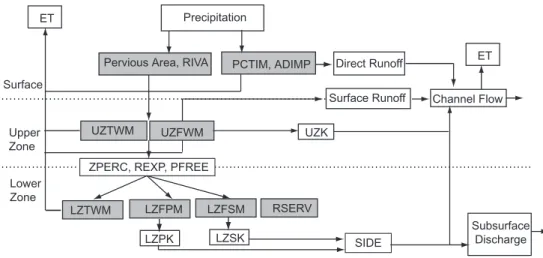
different speeds following Darcy’s law. The maximum storages for these different types of lower zone free water are the lower zone maximum tension water (LZTWM), the primary free water (LZFPM), and the supplemental free water (LZFSM). SAC-SMA’s processes and parameters are illustrated in more detail in Fig. 2. It is indicated in the figure that there are four principal forms of runoff generated by SAC-SMA: 1) direct

15

runoff on the impervious area, 2) surface runoff when the upper zone free water stor-age is filled and the precipitation intensity is greater than percolation and interflow rate, 3) the lateral interflow from upper zone free water storage, and 4) primary baseflow. The direct runoff is composed of the impervious runoff over the permanent impervious area and the direct runoff on the temporal impervious area. The permanent

impervi-20

ous area, represented by parameter PCTIM (percent of impervious area), represents constant impervious areas such as pavements. The temporal impervious area, repre-sented by parameter ADIMP (additional impervious area), includes the filling of small reservoirs, marshes, and temporal seepage outflow areas which become impervious when the upper zone tension water is filled. Prior work (Peck,1976) has shown that

25

thirteen out of sixteen parameters control model performance and must be calibrated. Feasible ranges of these thirteen parameters are presented byBoyle et al.(2000) and also used in the calibration studies ofTang et al.(2006b,a) andVrugt et al.(2003) (see Table2). As shown in Table 2, the maximum allowable value of ADIMP specified by

(17)

HESSD

Full Screen / Esc

EGU the author is 0.4 indicating that 40% of the watershed area is the temporal impervious

area, which can lead to large direct runoff under wet conditions.

4 Case study

4.1 Juniata watershed description

The Juniata Watershed, part of the Susquehanna River Basin, covers an area of

5

8800 km2 in the ridge and valley region of the Appalachian Mountains of south cen-tral Pennsylvania. The watershed is within the US NWS mid-Atlantic river forecast center (MARFC) area of forecast responsibility. The primary aquifer formations are composed of sedimentary and carbonate rocks that are presented in alternating lay-ers of sandstone, shale, and limestone. Approximately, 67 percent of the watlay-ershed

10

is forested, 23 percent is agricultural, 7 percent is developed area, and the rest is mine lands, water, or miscellaneous. There are 11 major sub-watersheds (see Fig. 3), among which, RTBP1, LWSP1, MPLP1, and NPTP1 have heavily controlled flows from reservoirs. Our preliminary analysis of the watershed focused on 7 headwater sub-watersheds where flows are not managed. Figure 5 illustrates our preliminary analysis

15

of the hydrologic conditions within the seven sub-watersheds by plotting their flow du-ration curves as well as monthly averages for streamflow, potential evapodu-ration, and precipitation. Figure 4 shows that the SPKP1 (Spruce Creek) and SXTP1 (Saxton) wa-tersheds have distinctly different flow regimes. In the remainder of our study, we have evaluated the model sensitivities within these two watersheds using the four sensitivity

20

analysis tools introduced in Sect. 2. As will be discussed in more detail in Sect. 5, our analysis evaluates model sensitivities for different temporal and spatial scales (i.e., SPKP1 and SXTP1 have drainage areas of 570 and 1960 km2, respectively).

(18)

HESSD

Full Screen / Esc

EGU 4.2 Data set

The SAC-SMA/SNOW-17 lumped model used required input forcing data consisting of precipitation, potential evapotranspiration (PE), and air temperature. The precipitation data are next generation radar (NEXRAD) multisensor precipitation estimator data from the US NWS. Hourly data for precipitation and air temperature were available from 1

5

January 2001 to 31 December 2003. The observed streamflow in the same period was obtained from United States Geological Survey (USGS) gauge stations located at the outlets of the SPKP1 and SXTP1 watersheds.

5 Computational Experiment

5.1 Model setup and parameterizations

10

In this study, we used a Linux computing cluster with 133 computer nodes composed of dual or quad AMD Opteron processors and 64 GB of RAM. Two month warmup periods (1 January to 28 Feburary 2001) were used to reduce the influence of initial conditions. Model performance was evaluated using three different time intervals (1 h, 6 h, 24 h) to test how parameter sensitivities change due to different prediction time scales. The a

15

priori parameter settings used for the SNOW-17 and SAC-SMA models where based on the recommendations of the Mid-Atlantic River Forecasting Center of the US NWS. The primary algorithmic parameters for PEST were set based on the recommenda-tions of Doherty (2004). The initial Marquardt lambda and its adjust factor were set to be 5 and 2 respectively. When calculating the derivatives, the parameters were

20

incremented by a fraction of the current parameters’ values subject to the absolute in-crement lower bounds. The fraction is 0.01 and the lower bounds vary from parameter to parameter based on their magnitudes. The parameter estimation process terminates if one of the following conditions is satisfied: 1) the number of iterations exceeds 30; 2) the relative difference between the objective value of the current iteration and the

(19)

HESSD

Full Screen / Esc

EGU minimum objective value achieved to date is less than 0.01 for 3 successive iterations;

3) the algorithm fails to lower the objective value over 3 successive iterations; 4) the magnitude of the maximum relative parameter change between optimization iterations is less than 0.01 over 3 successive iterations.

Statistical sample sizes are key parameters for RSA, ANOVA, and Sobol’s method.

5

In this study, the sample sizes were configured based on both literature recommenda-tions and experiments by observing the convergence and reproducibility of the sensi-tivity analysis results. Sieber and Uhlenbrook (2005) used a sample size of 10 times the number of perturbed parameters while doing sensitivity analysis on a distributed catchment model using LHS. However, the experimental analysis showed this is far

10

from enough for our study. Examining statistical convergence as a function of increas-ing sample size, we determined a size of 10 000 was sufficient for LHS in RSA. For the ANOVA method, typically the F-values increase for the sensitive parameters with increases in sample size (Mokhtari and Frey,2005). Our analysis of convergence for the ANOVA method’s F-values and parameter sensitivity rankings showed that a

sam-15

ple size of 10 000 was sufficient when using IFFD sampling. For Sobol’s quasi-random sequenceSobol’(1967) states that additional uniformity can be obtained if the sample size is increased according to the function n=2k, where k is an integer. Building on this recommendation, our analysis showed that Sobol’s sensitivity indices converged and were reproducible using a sample size 8192 (213).

20

5.2 Objective functions

Two different model performance objective functions were used to screen the sensitivity of SAC-SMA and SNOW17 for high streamflow and low streamflow. The first objective was the non-transformed root mean square error (RMSE) objective, which is largely dominated by peak flow prediction errors due to the use of squared residuals. The

25

second objective was formulated using a Box-Cox transformation of the hydrograph (z=[(y+1)λ−1]/λ where λ=0.3) as recommended byMisirli et al.(2003) to reduce the impacts of heteroscedasticity in the RMSE calculations (also increasing the influence

(20)

HESSD

Full Screen / Esc

EGU of low flow periods).

5.3 Bootstrap confidence intervals

For ANOVA and Sobol’s method, the F-values and sensitivity indices can have a high degree of uncertainty due to random number generation effects (Archer et al.,1997; Fieberg and Jenkins,2005). In this study, we used the bootstrap method (Efron and

5

Tibshirani,1993) to provide confidence intervals for the parameter sensitivity rankings for both ANOVA and Sobol’s method. Essentially, the samples generated by IFFD or Sobol’s sequence were resampled N times when calculating the F-values or sensitivity indices for each parameter, resulting in a distribution of the F-values or indices. The moment method (Archer et al.,1997) was adopted for acquiring the bootstrap

confi-10

dence intervals (BCIs) for this paper. The moment method is based on large sample theory and requires a sufficiently large resampling dimension to yield symmetric 95% confidence intervals. In this study, the resample dimension N was set to 2000 based on prior literature discussions as well as computational experiments that confirmed a symmetric distribution for standard errors. Readers interested in detailed descriptions

15

of the bootstrapping method used in this paper can reference the following sources (Archer et al.,1997;Efron and Tibshirani,1993).

5.4 Evaluation of sensitivity analysis results

As argued byAndres(1997), good sensitivity analysis tools should generate repeatable results using a different sample set to evaluate model sensitivities. The effectiveness

20

of a sensitivity analysis method refers to its ability to correctly identify the influential parameters controlling a model’s performance. Building on Andres (1997), we have tested the effectiveness of each of the sensitivity methods using an independent LHS-based random draw of 1000 parameter groups for the 18 parameters analyzed in this study.

25

(21)

sensitiv-HESSD

Full Screen / Esc

EGU ity analysis methods were combined to develop three parameter sets. Set 1 consists of

the full randomly generated independent sample set of 1000 parameter groups. In Set 2, the parameters classified as highly sensitive or sensitive are set to a priori values while the remaining insensitive parameters are allowed to vary randomly. Lastly, in Set 3 the parameters classified as being highly sensitive or sensitive vary randomly and

5

the insensitive parameters are set to a priori values.

Varying parameters that are correctly classified as insensitive in Set 2 should the-oretically yield a zero correlation with the full random sample of Set 1 (i.e., plot as a horizontal line). If some parameters are incorrectly classified as insensitive then the scatter plots show deviations from a horizontal line and increased correlation coe

ffi-10

cients (e.g., see Fig. 10a). Conversely, if the correct subset of sensitive parameters is sampled randomly (i.e., Set 3) than they should be sufficient to capture model output from the random samples of the full parameter set in Set 1 yielding a linear trend with an ideal correlation coefficient of 1. We extended the evaluation methodology of An-dres (1997) by calculating the corresponding correlation coefficients instead of using

15

scatter plots.

6 Results

Sections6.1–6.4 present the results attained for each of the four sensitivity analysis methods tested in this study. Results are presented for the SPKP1 and SXTP1 water-sheds at 1 h, 6 h, and 24 h timescales. Section 6.5 then provides a detailed analysis

20

of how the results from each sensitivity method compare in terms of their selection of highly sensitive, sensitive, and insensitive parameters for the SAC-SMA/SNOW-17 lumped model. Additionally, Sect.6.5builds on the work ofAndres(1997) to evaluate the relative effectiveness of the methods in identifying the key input parameters control-ling model performance. Detailed conclusions on how individual watershed properties

25

impact model performance are beyond the scope of this paper.

(22)

sev-HESSD

Full Screen / Esc

EGU eral ways that sensitivity analysis methods can be evaluated and used in the context

of watershed model identification and evaluation. The current study builds on the opti-mization research ofTang et al.(2006b) by focusing on how well PEST, RSA, ANOVA, and Sobol’s method can identify the set of model input parameters that control model performance. Successful screening of the relative importance of input parameters and

5

their interactions can help to limit the dimensionality of calibration search problems and serve to enhance the efficiency of uncertainty analysis. Recall from Sect.5 that the model performance objectives used in this study evaluate the influence of high stream-flow conditions via the RMSE measure and low streamstream-flow conditions via the Box-Cox transformed RMSE (TRMSE). Small values of these measures implies that the

SAC-10

SMA/SNOW-17 streamflow projections closely match observations in the simulated period.

6.1 Sensitivity results for PEST

In the case of PEST, sensitivities are computed using the Jacobean derivative-based composite measures defined in Eq. (1). The method is termed local because the

com-15

posite derivatives are evaluated at a single point in the parameter space deemed locally optimal by the Gauss-Marquardt-Levenberg algorithm. Tables3and4provide the sen-sitivities computed by PEST for the RMSE and TRMSE objectives, respectively. In the tables, highly sensitive parameters are designated with dark grey shading, sensitive parameters have light grey shading, and insensitive parameters are not shaded. The

20

SNOW-17 and SAC-SMA parameters are listed separately as are the 1 h, 6 h, and 24 h results for each watershed.

As a caveat, the thresholds used to differentiate highly sensitive, sensitive, and in-sensitive parameters are based only on the relative magnitudes of the derivatives given in each column, making them subjective and somewhat arbitrary. The thresholds were

25

determined by ranking each column in ascending order and then plotting the relative magnitudes of the derivatives. Results were classified as either highly sensitive or sensitive where the derivative values changed the most significantly. Insensitive

(23)

pa-HESSD

Full Screen / Esc

EGU rameters had small derivative values that could not be distinguished. Note different

thresholds were used for Tables3and4since the Box-Cox transformation reduced the original range of RMSE by approximately an order of magnitude. The results in Tables3 and4show that PEST did not detect significant changes in parameter sensitivities for high flow (RMSE) versus low flow (TRMSE) conditions. Also differences in the

time-5

scales of predictions as well as watershed locations did not significantly change the PEST sensitivity designations in both tables. Overall PEST found the parameters for impervious cover (PCTIM, ADIMP) and those for storage depletion rates (UZK, LZPK, LZSK) significantly impacted model performance, especially for daily time-scale predic-tions. The mean water-equivalent threshold for snow cover (SI) and lower zone storage

10

parameters (LZTWM, LZFSM, and LZFPM) were classified by PEST as being the least sensitive.

6.2 RSA Results

As described in Sect.2.2.2, a visual extension of RSA (Young,1978;Hornberger and Spear,1981;Freer et al.,1996;Wagener and Kollat,2006) was used to evaluate

pa-15

rameter sensitivities for the SAC-SMA/SNOW-17 lumped model. Results were com-puted for the same timescales and watersheds as were presented for PEST. Given the large number of results analyzed, Figs. 5 and 6 provide sample plots for our RSA analysis, whereas the full sensitivity classifications are summarized in Tables5and6. In Figs. 5 and 6 each model parameter has its own plot with its range on the horizontal

20

axis and its cumulative normalized RMSE distribution value on the vertical axis. In the plots, color shading is used to differentiate the likelihoods of each one of the ten bins used to divide the input parameter samples. High likelihood bins plotted in purple rep-resent portions of the parameters’ ranges where low RMSE values are expected. In the context of sensitivity analysis, RSA measures the distribution of model responses

25

that result from the 10 000 Latin hypercube input parameter groups sampled. When parameters are insensitive (see the SNOW-17 results shown in Fig. 5) each of the 10 sample bins plot over each other in linear trend lines that are representative of

(24)

uni-HESSD

Full Screen / Esc

EGU formly distributed RMSE values. Sensitive parameters produced highly dispersed bin

lines such as those shown for ADIMP shown in Fig. 6.

The SAC-SMA/SNOW-17 sensitivity classifications resulting from RSA are presented in Tables5 and6. The classifications represent our qualitative interpretation of visual plots similar to those in Figs. 5 and 6 for each timescale and each watershed. As is

5

standard in hydrologic applications of RSA (e.g.,Freer et al.,1996;Wagener and Kol-lat, 2006), only individual parameter impacts on model performance are considered and parameter interactions have been neglected. Analysis of Tables 5 and 6 show significant changes in sensitivity when comparing across timescales, watersheds, and model performance objectives. Examples of these changes include the increased

im-10

portance of the SNOW-17 parameters for gage precipitation adjustment factor (SCF) and minimum melt factor in non-rain periods (MFMIN) at the daily timescale. High flow and low flow conditions in both watersheds impacted RSA classification’s of highly sen-sitive parameters. The RMSE measure (i.e., high flow) identified additional impervious area (ADIMP) as the most sensitive parameter in tested cases. Shifting the focus to

15

low flow using the TRMSE measure resulted in the vadose zone storage (LZTWM) as being classified as the most sensitive parameter.

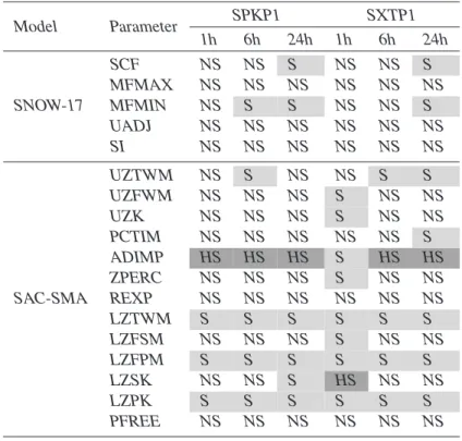
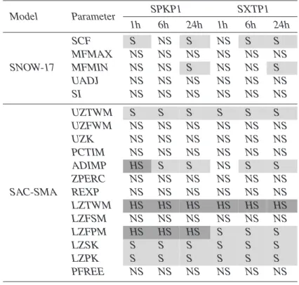
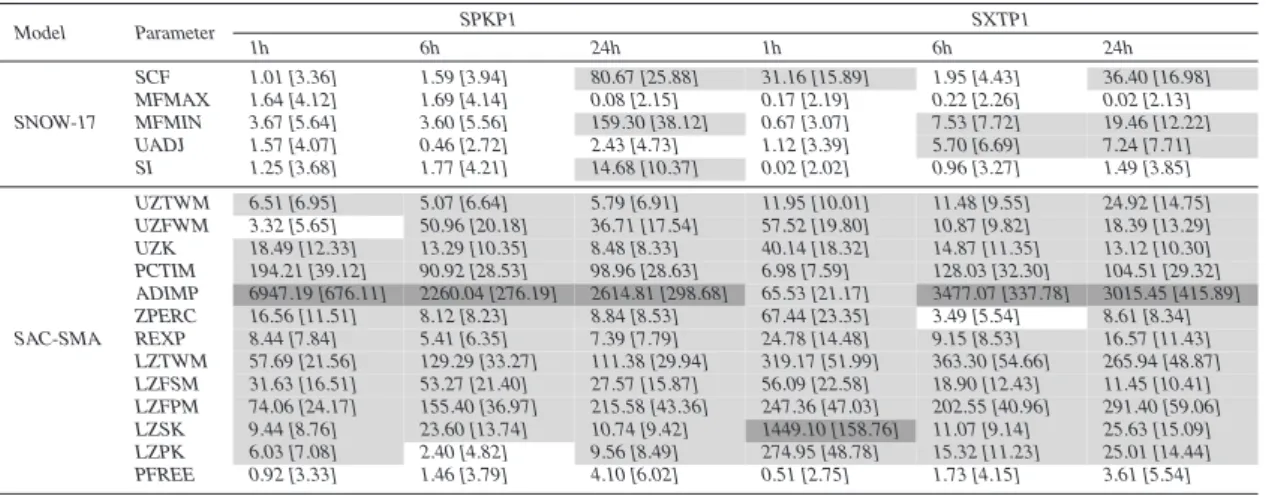
6.3 Sensitivity results for ANOVA

Recall that ANOVA is a parametric analysis of variance that uses the assumption of normally distributed model responses (RMSE and TRMSE for streamflow in this study)

20

to partition variance contributions between single parameters and parameter interac-tions. In this study, a second order ANOVA model (i.e., a model that considers pair wise parameter interactions) was fit to the model outputs and the F-test is used to evaluate the statistical significance of each parameter’s or parameter interaction’s impact on the model output. Higher F-values indicate higher significance or sensitivity. Additionally,

25

the coefficient of determination R2can be used to measure if incorporating parameter interactions into the ANOVA model improves its ability to represent model output vari-ability (Mokhtari and Frey,2005). Because random sampling can introduce significant

(25)

HESSD

Full Screen / Esc

EGU uncertainty into the calculation of F-values, we have followed the recommendations of

Archer et al. (1997) and used statistical bootstrapping to provide 95% confidence in-tervals for our ANOVA sensitivity rankings. Tables7 and 8 provide F-values for each parameter as well as its bootstrapped confidence interval. Tabular presentation of the ANOVA results improved their clarity since the F-values ranged over 4 orders of

mag-5

nitude [0.02–7000] making plots difficult to interpret.

Tables7and8are formatted similarly to the prior sensitivity tables where highly sen-sitive parameters have dark grey shading, sensen-sitive parameters have light grey shad-ing, and insensitive parameters have no shading. These classifications were based on the F-distribution where a threshold of 4.6 represents less than a 1-percent chance of

10

misclassifying a parameter as sensitive. As can be seen in the tables, some param-eters’ F-values were up to three orders of magnitude larger than 4.6. A threshold of 460 was used to classify parameters as being highly sensitive. Although the threshold used to classify highly sensitive parameters is subjective, it accurately captures those parameters with very large F-values.

15

Analysis of Table7shows that for the high-flow RMSE objective, the most significant differences in sensitivities across timescales and across watersheds involved SNOW-17 parameters. The results show increasing sensitivities for the snow accumulation gage precipitation adjustment factor (SCF) and the minimum melt factor for non-rain periods (MFMIN) at the daily timescale. Overall, Table7shows that most of SAC-SMA

20

parameters are sensitive for high flow conditions regardless of timescale or watershed. The high flow RMSE analysis identified additional impervious area (ADIMP) as having the highest influence on model variance while percolation of free water (PFREE) is rated to have the least impact.

In Table8 the ANOVA results using the low flow TRMSE objective are substantially

25

different from those for high flow in Table7. There is a pronounced difference between ANOVA predicted sensitivities for the two watersheds for the low-flow measure. For the SPKP1 watershed most of the SAC-SMA parameters remain sensitive across all tested timescales, whereas parameters describing upper zone storage and flows (UZFWM,

(26)

HESSD

Full Screen / Esc

EGU UZK, PCTIM) are classified as insensitive for SXTP1. As would be expected for low

flows, Table8 shows a general reduction relative to Table 7in the influence of upper zone parameters and an increase in the importance lower zone parameters.

Beyond single parameter sensitivities, the coefficients of determination in Table 9 show that 2nd order interactions (or pair wise parameter interactions) improve the

ac-5

curacy of the ANOVA model, which means the model better represents the total vari-ance of the SAC-SMA/SNOW-17 model output. The coefficients of determination show that 2nd order parameter interactions improve the ANOVA models’ performances by up to 50%. Figure 7 illustrates the 2nd order parameter interactions impacting the SAC-SMA/SNOW-17 model. Second order analysis changes the degrees of freedom

10

used when analyzing the F-distribution making it necessary to define a new threshold in Fig. 7. An F-value threshold of 3.32 designates at least a 99% likelihood of being sensitive. Again higher F-values imply higher sensitivity.

Figure 7 provides a more detailed portrayal of how parameter sensitivities change across timescales for each of the watershed models. The RMSE-based ANOVA

inter-15

actions in Fig. 7a for the SPKP1 watershed show that lower zone parameter interac-tions are increasingly more important for longer timescale, whereas the opposite trend is present for the SXTP1 watershed. These plots imply each watershed model has a “unique” set of parameter interactions impacting its performance (Beven,2000).

The uniqueness of each watershed model is further supported by the TRMSE results

20

shown in Fig. 7b. As expected lower zone parameter interactions are important for predicting low-flows for both watersheds. Interestingly, all of the low-flow predictions for the SPKP1 watershed are heavily impacted by parameter interactions, more so than any of the other cases analyzed using the ANOVA method.

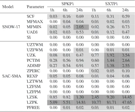
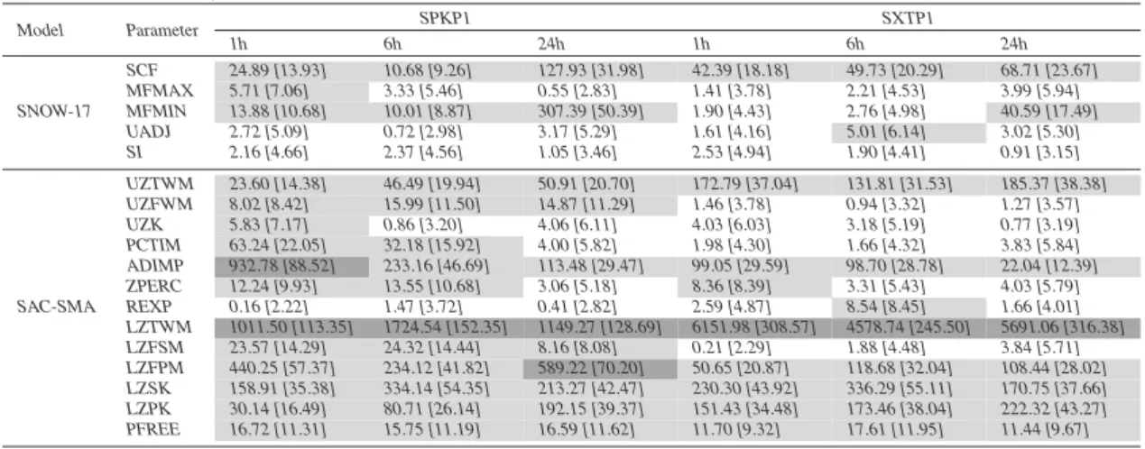
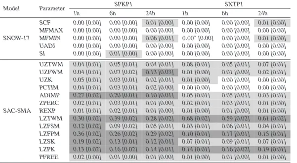
6.4 Sensitivity results for Sobol’s method

25

Recall from Sect.2.2.4, that Sobol’s method decomposes the overall variance of the sampled SAC-SMA/SNOW-17 model output to compute 1st order (single parameter), 2nd order (two parameter), and total order sensitivity indices. These indices are

(27)

pre-HESSD

Full Screen / Esc

EGU sented as percentages and have straightforward interpretations as representing the

percent of total model output variance contributed by a given parameter or parameter interaction. The total order indices are the most comprehensive measures of a single parameter’s sensitivity since they represent the summation of all variance contributions involving that parameter (i.e., its 1st order contribution plus all of its pair wise

interac-5

tions).

Table 10 shows the relative importance of 1st and 2nd order effects for all of the cases analyzed. Readers should note that the truncation and Monte Carlo approxi-mations of the integrals required in Sobol’s method can lead to small numerical errors (e.g., seeArcher et al.,1997;Sobol’,2001;Fieberg and Jenkins,2005) such as slightly

10

negative indices or for example in Table10the few cases where 1st and 2nd order ef-fects sum to be slightly larger than 1. In this study these effects were very small and did not impact parameter rankings. Table 10 supports our analysis assumption that 1st and 2nd order parameter sensitivities explain nearly all of the variance in the SAC-SMA/SNOW-17 model’s output distributions. The table also shows that the importance

15

of 2-parameter interactions ranged from 9% to 40% of the total variance depending on the model performance objective, the prediction timescale, and the watershed.

Tables11and12summarize the total order indices (i.e., total variance contributions) for the SAC-SMA/SNOW-17 parameters analyzed. Again highly sensitive parameters are designated with dark grey shading, sensitive parameters have light grey shading,

20

and insensitive parameters are not shaded. In all of the results presented for Sobol’s method, parameters classified as highly sensitive had to contribute on average at least 10-percent of the overall model variance and sensitive parameters had to contribute at least 1-percent. These thresholds are subjective and their ease-of-satisfaction de-creases with increasing numbers of parameters or parameter interactions. In Tables11

25

and 12 the total order indices again show that the model performance objective, the prediction timescale, and the watershed all heavily impact the SAC-SMA/SNOW-17 sensitivities.

(28)

vari-HESSD

Full Screen / Esc

EGU ance of the simulation model’s output. Only the minimum melt factor for non-rain

pe-riods (MFMIN) parameter has a statistically reliable sensitivity when the bootstrapped confidence intervals are considered. Tables11and12 also insinuate that most of the SAC-SMA model parameters are sensitive. For the high-flow RMSE results, the up-per zone free water storage (UZFWM) and the additional imup-pervious area (ADIMP)

5

were the most sensitive SAC-SMA parameters. The lower zone storage parameters dominate model response for the low-flow TRMSE measure. In particular, the tension water storage (LZTWM) appears to be the dominant overall parameter, especially for the SXTP1 watershed’s results where it explains 60% of the output’s variance.

Figure 8 provides a more detailed understanding of the total order indices presented

10

in Tables11and12. Similar to the ANOVA interaction plots in Sect.6.3, these figures show the matrix of parameter interactions where circles designate pairings that con-tribute at least 1% of the overall model output variance. The actual 2nd order indices’ values are shown with the color shading defined in the plots’ legends. These plots show how the dominant parameters for both the RMSE and TRMSE results tend to

15

have the greatest number of interactions (e.g., ADIMP and UZFWM in Fig. 8). Inter-estingly, there are very distinct differences for the parameter interactions for the two watersheds. Recall from Table10that the SXTP1 hourly RMSE results had the largest contribution from 2nd order effects (44% of the total variance). Both Table11and the interactions shown in Fig. 8a confirm the increased importance of interactions,

partic-20

ularly interactions with lower zone parameters. When comparing the RMSE results in Fig. 8a with TRMSE results in Fig. 8b the shift from high-flow to low flow analysis tends to increase the importance interactions with lower zone parameters for the SPKP1 wa-tershed, whereas the opposite is true for the SXTP1 watershed. Readers should note that our 1% threshold for Sobol’s method is particularly conservative when analyzing

25

Figs. 8a and b since the number of variables analyzed increases from 18 for 1st order analysis to 162 parameter interactions in 2nd order analysis.

(29)

HESSD

Full Screen / Esc

EGU 6.5 Comparative summary of sensitivity methods

Sections6.1–6.4present classifications of SAC-SMA/SNOW-17 model parameters into three categories: (1) highly sensitive, (2) sensitive, and (3) insensitive. Given the large number of cases analyzed in this study, Fig. 9 was developed to provide a compara-tive summary of the results attained from the four sensitivity analysis methods. These

5

figures show that there are distinct similarities and differences between the sensitiv-ity classifications attained using each method. For example, despite the subjective decisions required to differentiate highly sensitive and sensitive parameters, generally RSA, ANOVA, and Sobol’s method agree on their classifications of the most sensitive parameters for each scenario.

10

All four sensitivity methods show that the SAC-SMA/SNOW-17 model’s responses are “uniquely” determined by the performance objective specified, prediction timescale, and specific watershed being modeled (Beven,2000). Differences between the four sensitivity methods’ classifications as illustrated in Fig. 9 are particularly pronounced for parameters at the threshold between sensitive and insensitive. One of the biggest

15

discrepancies shown in the plots is that PEST generally found the SNOW-17 parame-ters to be sensitive for hourly and 6-hourly predictions. None of the global sensitivity methods showed a similar result, making it likely that the PEST results are reflective of local optima in the model’s response surface, which would be expected to be highly multimodal (Duan et al.,1992;Tang et al.,2006b).

20

Figure 9 shows that RSA generally defined the smallest subset of SAC-SMA/SNOW-17 parameters as being sensitive or highly sensitive. The RSA version used in this study is unique among the four tested sensitivity methods in the sense that our clas-sifications required qualitative assessments of a visual representation of results. As noted above RSA yields very similar rankings for highly sensitive results, but the

quali-25

tative interpretation of sensitivity becomes more challenging for parameters that show modest sensitivity.

(30)

HESSD

Full Screen / Esc

EGU the four sensitivity methods, it does not allow for any quantitative analysis of their

rel-ative effectiveness as screening tools. Building onAndres(1997), we have tested the effectiveness of each of the sensitivity methods used in this study. We have used the sensitivity classifications given in Fig. 9 in combination with an independent LHS-based random draw of 1000 parameter groups for the 18 parameters analyzed in this study.

5

Recall from Sect.5.4, that the independent sample and the sensitivity classifications in Fig. 9 were used to develop three parameter sets. Set 1 consists of the full ran-domly generated independent sample set. In Set 2, the parameters classified as highly sensitive or sensitive are set to a priori fixed values while the remaining insensitive parameters are allowed to vary randomly. Lastly, in Set 3 the parameters classified as

10

being highly sensitive or sensitive vary randomly and the insensitive parameters are set to a priori values.

Figure 10 illustrates that by plotting Set 2 versus Set 1 as well as Set 3 versus Set 1 we can test the effectiveness of the sensitivity analysis methods. As shown for the Sobol method’s results in Fig. 10a varying parameters that are correctly classified as

15

”insensitive” in Set 2 should theoretically yield a zero correlation with the full random sample of Set 1 (i.e., plot as a horizontal line). If some parameters are incorrectly classified as insensitive then the scatter plots show deviations from a horizontal line and increased correlation coefficients as is the case for the PEST, RSA, and ANOVA results in Fig. 10a. Conversely, if the correct subset of sensitive parameters is sampled

20

randomly (i.e., Set 3) than they should be sufficient to capture model output from the random samples of the full parameter set in Set 1 yielding a linear trend with an ideal correlation coefficient of 1. Figure 10b shows that the Sobol’s method yields the highest correlation between Set 3 and Set 1 followed closely by ANOVA. Interestingly, PEST and RSA yield similar correlations for the SPKP1 watershed’s results shown in Fig. 10.

25

More generally, the plots in Fig. 10 show that this analysis can be quantified using correlation coefficients.

Table13provides a summary of correlation coefficients for all of the test cases an-alyzed in this study. Although PEST shows the worst performance overall, it is