HAL Id: insu-03040609
https://hal-insu.archives-ouvertes.fr/insu-03040609
Submitted on 19 Mar 2021
HAL is a multi-disciplinary open access
archive for the deposit and dissemination of
sci-entific research documents, whether they are
pub-lished or not. The documents may come from
teaching and research institutions in France or
abroad, or from public or private research centers.
L’archive ouverte pluridisciplinaire HAL, est
destinée au dépôt et à la diffusion de documents
scientifiques de niveau recherche, publiés ou non,
émanant des établissements d’enseignement et de
recherche français ou étrangers, des laboratoires
publics ou privés.
between satellite, reanalysis, and local-scale observations
C. Di Biagio, Jacques Pelon, Y. Blanchard, Lilian Loyer, Stephen R. Hudson,
V.P. Walden, Jean-Christophe Raut, S. Kato, Vincent Mariage, Mats
Granskog
To cite this version:
C. Di Biagio, Jacques Pelon, Y. Blanchard, Lilian Loyer, Stephen R. Hudson, et al.. Towards a better
surface radiation budget analysis over sea ice in the high Arctic Ocean: a comparative study between
satellite, reanalysis, and local-scale observations. Journal of Geophysical Research: Atmospheres,
American Geophysical Union, 2021, 126 (4), pp.e2020JD032555. �10.1029/2020JD032555�.
�insu-03040609�
1. Introduction
The Arctic is experiencing the fastest and most evident climate change on Earth (Serreze & Barry, 2011). Clouds and surface properties both play a crucial role in the surface energy budget of this region, as they determine the amount of shortwave (SW) and longwave (LW) radiation in the lower atmosphere. The water content in super-cooled boundary layer clouds is also of particular importance for the Arctic region (e.g., Pithan et al., 2018) as atmospheric circulation patterns may be changing (Graham et al., 2017b). The surface energy budget, in turn, affects sea ice growth and melt, evaporation, atmospheric structure, and stability, with consequences for regional and large-scale meteorology and climate (Bintanja & Krikken, 2016; Bouras-sa et al., 2013; Döscher et al., 2014). However, due to present day limitations in observations and atmospher-ic reanalysis, understanding and predatmospher-icting climate change over this sensitive region still remains limited (Kay et al., 2016).
Both satellite and reanalysis products are often used for Arctic energy budget studies and aim to accurately represent cloud fraction, distribution and microphysical properties, as well as surface properties. However, it has been shown that both satellite-retrieved and model-simulated surface SW and LW radiation fields are largely biased in different seasons at high latitudes (Zygmuntowska et al., 2012; Kay & L'Ecuyer, 2013; Liu & Key, 2016; Lenaerts et al., 2017; Graham et al., 2017a, 2019). Biases in satellite products, such as the Clouds and the Earth's Radiant Energy System Energy Balanced and Filled (CERES-EBAF) as well as the Synoptic
Abstract
Reanalysis datasets from atmospheric models and satellite products are often used for Arctic surface shortwave (SW) and longwave (LW) radiative budget analyses, but they suffer from limitations and require validation against local-scale observations. These are rare in the high Arctic, especially for longer periods that include seasonal transitions. In this study, radiation and meteorological observations acquired during the Norwegian Young Sea Ice Cruise (N-ICE2015) campaign over sea ice north of Svalbard (80–83°N, 5–25°E) from January–June 2015, cloud lidar observations from the Ice-Atmosphere-Ocean Observing System and the Cloud and Aerosol Lidar with Orthogonal Polarization are compared to daily and monthly satellite retrievals from the Clouds and the Earth's Radiant Energy System (CERES) and ERA-Interim and ERA5 reanalysis. Results indicate that surface temperature is a significant driver for winter LW radiation biases in both satellite and reanalysis data, along with cloud optical depth in CERES. In May, the SW and LW downwelling irradiances are close to observations and cloud properties are well captured (except for ERA-Interim), while SW upward irradiances are biased low due to surface albedo biases in all datasets. Net SW and LW radiation biases are comparable (∼20–30 Wm−2) but opposite in signfor ERA-Interim and CERES in May, which allows for error compensation. Biases reduce to ±10 Wm−2
in ERA5. In June downward LW remains biased low (8–10 Wm−2) in all datasets suggesting unsettled
cloud representation issues. Surface albedo always differs by more than 0.1 between datasets, leading to significant SW and total flux differences.
© 2020. American Geophysical Union. All Rights Reserved.
Study Between Satellite, Reanalysis, and local-scale
Observations
C. Di Biagio1,2 , J. Pelon2, Y. Blanchard3 , L. Loyer2, S. R. Hudson4 , V. P. Walden5 , J.-C. Raut2 , S. Kato6 , V. Mariage2, and M. A. Granskog4
1LISA, UMR CNRS 7583, Université Paris-Est-Créteil, Université de Paris, Institut Pierre Simon Laplace (IPSL), Créteil, France, 2LATMOS/IPSL, Sorbonne Université, Université Versailles Saint Quentin, CNRS, Paris, France, 3Centre pour l’Étude et la Simulation Du Climat à l’Échelle Régionale (ESCER), Université Du Québec à Montréal, Montréal, Québec, Canada, 4Norwegian Polar Institute, Fram Centre, Tromsø, Norway, 5Department of Civil and Environmental Engineering, Washington State University, Pullman, WA, USA, 6NASA Langley Research Center, Hampton, VA, USA
Key Points:
• Surface albedo, temperature, and cloud properties contribute to bias Clouds and the Earth's Radiant Energy System (CERES) and ERA-Interim surface irradiances, while ERA5 performs better
• In spring ERA-Interim and CERES SW and LW biases compensate allowing estimates of total surface radiation to agree with surface observations
• Differences up to 0.1 in gridded surface albedo remain between the datasets and affect shortwave and total surface radiation budgets
Supporting Information: • Supporting Information S1 Correspondence to: C. Di Biagio, [email protected] Citation:
Di Biagio, C., Pelon, J., Blanchard, Y., Loyer, L., Hudson, S. R., Walden, V. P. et al. (2021). Toward a better surface radiation budget analysis over sea ice in the high Arctic Ocean: a comparative study between satellite, reanalysis, and local-scale observations. Journal
of Geophysical Research: Atmospheres, 126, e2020JD032555. https://doi. org/10.1029/2020JD032555 Received 6 FEB 2020 Accepted 15 NOV 2020 Author Contributions: Conceptualization: C. Di Biagio, J. Pelon
Data curation: S. R. Hudson,
V. P. Walden, V. Mariage
Formal analysis: C. Di Biagio, J. Pelon,
Y. Blanchard, L. Loyer, V. Mariage
Funding acquisition: J. Pelon, S. R.
Hudson, V. P. Walden, M. A. Granskog
Investigation: S. R. Hudson,
V. P. Walden, V. Mariage, M. A. Granskog
Methodology: C. Di Biagio, J. Pelon,
Y. Blanchard, L. Loyer, S. R. Hudson, V. P. Walden, J.-C. Raut, M. A. Granskog
Project administration: J. Pelon,
TOA (Top-of-Atmosphere) and surface fluxes and clouds (CERES-SYN) products, appear to be quite signif-icant in relation to cloud frozen water (CFW; Lenaerts et al., 2017). The fixed satellite overpass time and low spatial resolution may also contribute to biases in observations, but this problem is expected to be less critical in the Arctic, which experiences more frequent satellite overpasses than lower latitudes. Addition-ally, the assumptions made for retrieval algorithms (e.g., vertical cloud distribution) and/or the specifica-tion of surface albedo can be crude in terms of the regional and seasonal changes of ice and snow-covered surfaces in satellite products (e.g., Blanchard et al., 2014; Van Tricht et al., 2016). On the other hand, the ERA-Interim reanalysis dataset (Dee et al., 2011), that is, the global atmospheric reanalysis produced by the European Center for Medium-Range Weather Forecasts (ECMWF), has been shown to overestimate surface temperature and underestimate cloud liquid water (CLW) amount over the polar ocean in winter and spring (Graham et al., 2019; Lenaerts et al., 2017; Sedlar, 2018; Zygmuntowska et al., 2012) and, to a smaller extent, the CFW in similar conditions (Lenaerts et al., 2017). Recently the new ERA5 reanalysis was also produced by ECMWF, bringing several improvements in terms of resolution and overall quality, as for example, in sea surface temperature and sea ice parameters (Hersbach et al., 2019, 2020). Nevertheless, surface temperature bias (in winter) over sea ice still a concern in ERA5 (Wang et al., 2019).
The improvement of satellite and reanalysis products through a better representation of processes in mete-orological models, is a primary objective of the A-Train space-borne observatory (https://atrain.nasa.gov/, Stephens et al., 2018). For example, the combination of such data has already been used to improve the parametrization of super-cooled boundary-layer water clouds at high latitudes (Forbes et al., 2016). None-theless, due to specific Arctic surface properties, improving satellite and reanalysis products requires having accurate surface-based field observations to compare with (Blanchard et al. 2014; Liu et al. 2017). Such observations are challenging and are mostly limited to the International Arctic Systems for Observing the Atmosphere coastal stations in the high Arctic (Uttal et al., 2016) and to a few sets of observations from dedicated field experiments and long-term stations over the Arctic region (e.g., Di Biagio et al., 2012). The first intensive field campaign documenting the cloud, albedo, and radiation fields and their coupled var-iations over a full-year period over the Arctic Ocean was the Surface HEat Budget of the Arctic (SHEBA) experiment, which occurred from October 1997 to October 1998 (Intrieri et al., 2002; Perovich et al., 2002; Persson et al., 2003; Shupe & Intrieri, 2004). Most of the campaigns following SHEBA were performed dur-ing summer when ship-based access is easiest (for example, the Arctic Sumer Cloud Ocean Study, ASCOS, [Tjenström et al., 2014], the Arctic Clouds in Summer Experiment, ACSE, [Sotiropoulou et al., 2016], and the measurements performed from the Tara vessel [Riihelä et al., 2017; Vihma et al., 2008]).
The Norwegian young sea Ice cruise (N-ICE2015, January–June 2015, http://www.npolar.no/en/projects/n-ice2015.html) is the most recent experiment to investigate processes linked to the younger and thinner Arc-tic sea ice during the winter to summer transition. Compared to SHEBA, N-ICE2015 was conducted in the more synoptically-active North Atlantic sector of the Arctic Ocean north of Svalbard. During N-ICE2015, observations of the atmosphere, ocean, ice dynamics, snow and ice physics, and marine ecosystem, includ-ing all components of surface SW and LW radiation and surface shortwave albedo, were performed (Gran-skog et al., 2018). Winter surface radiation data during N-ICE2015 showed a bimodal distribution of surface net (downward minus upward) LW flux comparable to that observed during SHEBA (Graham et al., 2017a). The two modes of the distribution correspond to clear-sky conditions (about −40 Wm−2) and cloudy
condi-tions (∼0 Wm−2) (Shupe & Intrieri, 2004). The radiatively clear state was shown to be usually prevalent
dur-ing the Arctic winter (Stramler et al., 2011). Furthermore, satellite data indicate that the two winter states are likely to operate over the entire Arctic basin (Cesana et al., 2012; Stramler et al., 2011), but both large scale and regional models inadequately represent the atmospheric vertical stability and transitions between them (Pithan et al., 2016). The analyses performed by Graham et al. (2017a, 2019) for N-ICE2015 showed that positive biases of about +20 W m−2 (monthly averages) were linked to surface temperature biases in the
ERA-Interim reanalysis with respect to ground-based observations.
During the N-ICE2015 field experiment, platforms from the Ice-Atmosphere-Arctic Ocean Observing System (IAOOS) project were deployed. The IAOOS network is the first ever ensemble of autonomous drifting buoys with both atmospheric and oceanic profiling instruments distributed over the high central Arctic, including the region north of 82°N (Provost et al., 2015). Other extensive programs of buoys deployment across the Arctic Ocean, such as the International Arctic Buoy Program (http://iabp.apl.washington.edu/index.html),
Resources: J. Pelon, M. A. Granskog Software: C. Di Biagio, Y. Blanchard,
L. Loyer, V. Mariage
Supervision: J. Pelon, M. A. Granskog Validation: C. Di Biagio
Visualization: C. Di Biagio
Writing – original draft: C. Di Biagio,
J. Pelon
Writing – review & editing:
C. Di Biagio, J. Pelon, Y. Blanchard, S. R. Hudson, V. P. Walden, J.-C. Raut, S. Kato, M. A. Granskog
were mostly focused on surface measurements over the past decades. Instead, the IAOOS buoys include a backscatter lidar system for cloud and aerosol profiling, surface meteorological sensors, snow and ice temperature profiler, and ocean profilers (Mariage et al., 2017; Provost et al., 2015). The IAOOS platforms were designed to perform regular year-round observations of the atmosphere, sea ice, and ocean composi-tion and structure, simultaneously. IAOOS lidar observacomposi-tions acquired during the Barneo 2014 campaign (October–December 2014) and during N-ICE2015 (Di Biagio et al., 2018; Mariage et al., 2017) were used to investigate the occurrence and distribution of winter to summertime clouds and aerosols in the high Arctic Ocean. It was shown that low-level clouds (below 2 km altitude) were very frequent north of Svalbard in spring (Di Biagio et al., 2018). The observed attenuation of lidar signals confirms that mixed phase clouds occur often as previously reported from SHEBA observations (Shupe et al., 2006) and over Arctic land sta-tions (Shupe, 2011).
In this study, the dataset of the radiation fluxes, surface albedo, meteorological parameters, and cloud oc-currence and properties from N-ICE2015 and IAOOS in the winter to summer 2015 period were used in combination with Cloud and Aerosol Lidar with Orthogonal Polarization (CALIOP) space-borne data to compare with state-of-the-art satellite and reanalysis datasets: the CERES-SYN, CERES-EBAF, ERA-Inter-im and the new ERA5 products. The goal is to evaluate the accuracy of these data sets, which are widely used in Arctic research, with local-scale observations and identify sources of discrepancies. First, the data and analysis methods are presented in Section 2, followed by results of the comparisons in Section 3. The observed differences between the measurements and CERES-SYN and EBAF retrievals and ERA-Interim and ERA5 reanalysis are discussed with the aid of the IAOOS and CALIOP observations in Section 4 before concluding the study.
2. Data and Methods
In the following subsections, the different datasets used in this study and their processing, including spatial and temporal colocation, are described. Uncertainty estimates for all used variables and details on their calculation are provided in Table S1 in the supporting information.
2.1. Ground-Based Observations
2.1.1. N-ICE2015 Radiation, Albedo and Meteorological Data
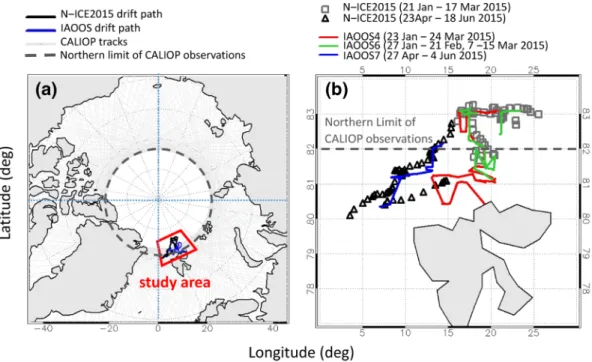
Atmospheric measurements during N-ICE2015 were performed at an ice camp installed about 300 m away from the Norwegian research vessel Lance as it drifted with the sea ice from January–June 2015 north of Svalbard (Cohen et al., 2017; Granskog et al., 2018; Kayser et al., 2017; Walden et al., 2017). Meteorological conditions were highly variable in winter, with the passage of several storms, but became more stable in spring and summer (Cohen et al., 2017; Walden et al., 2017). The vessel was navigated into the ice pack, moored sequentially to four different ice floes and drifted with them (Cohen et al., 2017). The drift path for N-ICE2015 during this study period is shown in Figure 1 and covers the region ∼80°–83°N latitude and ∼5°–25°E longitude. The drifting periods were 38 days for Floe 1 (15 January–21 February), 24 days for Floe 2 (24 February–19 March), 49 days for Floe 3 (18 April–15 June), and 16 days for Floe 4 (7–21 June). A break was taken from mid-March to mid-April to refuel and resupply. The first three floes started in the northern part of the Nansen basin whereas Floe 4 drifted closer to the ice edge (see Figure 1 in Granskog et al. (2018) showing the ice extent on the May 25, 2015 and the N-ICE2015 floe trajectories).
Radiative fluxes at the surface were measured on all four floes during N-ICE2015 (Hudson et al., 2016; Walden et al., 2017). Downward and upward SW and LW irradiances (SWdw, SWuw, LWdw, LWuw) were
meas-ured at 1 min resolution by Kipp & Zonen CMP22 and CGR4 radiometers (200–3,600 nm and 4.5–42 μm bandwidth, respectively), both equipped with a Kipp & Zonen CVF4 heating and ventilation unit. Each of the radiometers was calibrated by the manufacturer before and after the field campaign. The accuracy was 2% (or 5 W m−2) for global downward solar radiation, 3% for reflected solar radiation, and less than 3%
for downward and upward longwave fluxes (Walden et al., 2017). The height of the instruments above the snow surface was between 1 and 1.2 m on each of the floes throughout the experiment. The surface below the instruments was snow, so that the field of view of the upward instruments was always a snow-covered sea-ice surface.
The radiometers were checked daily to ensure that they were free of frost, rime, or moisture, and they were leveled and ventilated. A set of quality flags (QF) was developed for the data set (0-good data, 1-use with caution, and 2-bad data) (Walden et al., 2017). In our analysis, we considered only data with QF = 0 and eliminated days for which more than 30% of data had QF equal to 1 and 2. This removed 22 days of meas-urements, 12 of them in March, 2 in April, 4 in May, and 4 in June. Because of the need to reposition the ship when the floes broke up and the quality-control selection, the only almost complete month of radiation measurements was May (27 days). The other months have a fewer number of days of measurements: 11 (January), 19 (February), 4 (March), 6 (April), and 12 (June).
Surface broadband shortwave albedo (A) data, that is, the ratio of upward to downward SW irradiance meas-urements, were derived in springtime for a 3 h period centered around local noon (Walden et al., 2017). Radiation instruments were installed close to the weather mast providing complementary meteorological data of temperature, pressure, wind speed and direction (Hudson et al., 2015). Meteorological radiosondes were launched twice a day (at about 0 UTC and 12 UTC), either from the ice by the ship or from the ship's deck (Hudson et al., 2017; Kayser et al., 2017).
2.1.2. IAOOS Lidar Observations of Aerosols and Clouds
Three IAOOS lidar systems, identified as IAOOS 4, 6, and 7, working at ∼800 nm wavelength, were deployed in the region north of Svalbard during the N-ICE2015 campaign (see Figure 1). The IAOOS lidars profiled in the ∼60 m–15 km altitude range. Measurements were performed up to four times per day with a typical 10-min averaging sequence for each profile and a vertical resolution between 15 and 60 m. Calibration and data corrections (desaturation, geometrical factor and background corrections) were performed to derive the attenuated backscatter coefficient (βatt) and the integrated attenuated backscatter (IAB) according to the
anal-ysis by Mariage et al. (2017). Clouds, aerosols, blowing snow, precipitation or pristine molecular profiles were discriminated using IAOOS observations with an algorithm based on lidar signal strength presented by Di Biagio et al. (2018). Near-surface (1.5 m) temperature and surface pressure were measured on these platforms.
Figure 1. (a) Map showing the drift tracks of the N-ICE2015 ice camps and the three IAOOS buoys during the
January–June 2015 period. The CALIOP tracks north of 70°N are also shown. The red area indicates the study area. (b) Detail of the N-ICE2015 and IAOOS drift paths in a smaller region north of Svalbard archipelago. The N-ICE2015 ship positions are shown as daily averages. CALIOP, Cloud and Aerosol Lidar with Orthogonal Polarization; IAOOS, Ice-Atmosphere-Arctic Ocean Observing System; N-ICE2015, Norwegian young sea ICE 2015.
The IAOOS low level (<2 km) cloud fraction was determined from observations as a 5-days running average of cloud occurrence measured by the lidar system (see also Di Biagio et al., 2018). The cloud optical thick-ness (COT) at 800 nm was estimated from IAOOS observations as follows. For large cloud backscattering (e.g., high cloud reflectance) the cloud transmission can be assumed to be very low so that the IAB is nearly constant and only depends on the lidar extinction-to-backscattering ratio Sc, and the multiple scattering
factor η, as IAB = 1/(2ηSc) (Spinhirne et al., 1989). This allows the determination of the effective lidar
ex-tinction-to-backscattering ratio Sce = ηSc. The backscattering coefficient (β) can then be derived from the
attenuated backscattering coefficient by solving the lidar equation
att z z exp 2Sce 0z r dr
(1) using a forward calculation algorithm (Klett, 1985). The extinction coefficient was retrieved as
z Sc
z ,and the low cloud COT was equal to the product of the lidar ratio with the integrated backscatter coefficient:
max min z c zCOT S r dr for clouds from zmin = 0 up to an altitude zmax considered here to be equal to 2 km. A mul-tiple scattering factor η = 0.8, was considered here based on previous IAOOS lidar analyses (Mariage et al., 2017).
2.2. Satellite Observations 2.2.1. CALIOP Cloud Data
CALIOP data were considered in this study together with IAOOS surface observations to retrieve satellite information on cloud cover and vertical distribution (Winker et al., 2009). CALIOP is the primary instru-ment of the CALIPSO (Cloud-Aerosol Lidar and Infrared Pathfinder Satellite Observation) satellite. The CALIOP version 4.10 data products (Vaughan et al., 2017) were used. Data were available for the entire period of N-ICE2015. The cloud occurrence (%) for each day in the surrounding area of the N-ICE2015 measurement site was estimated as the ratio of the number of CALIPSO pixels with at least one cloud layer in the column to the total number of CALIPSO pixels in the region. The cloud occurrence was calculated for the whole 0–10 km altitude range and separately in the 0–2, 2–5, and 5–10 km altitude domains.
2.2.2. CERES-EBAF and CERES-SYN Radiation Data
Surface radiation data were derived from two CERES products: (i) the CERES-EBAF Surface Ed4.0 dataset (Kato et al., 2013) providing the monthly and climatological averages of surface clear-sky and all-sky upward and downward SW and LW fluxes and (ii) the SYN1deg-Day Edition 4.0 dataset (D. A. Rutan et al., 2015), hereafter referred as CERES-SYN, providing daily surface clear-sky and all-sky upward and downward SW and LW fluxes. Both datasets are over 1° by 1° global grid. In the retrieval algorithm, CERES TOA radiance measurements are converted into instantaneous SW and LW surface fluxes using scene-dependent angular directional models based on the Moderate Resolution Imaging Spectroradiometer (MODIS) retrievals of cloud properties and ancillary meteorological data from the Goddard Earth Observing System (GEOS) rea-nalysis product (version 5.4.1 in CERES-SYN).
The CERES-SYN surface irradiances are computed hourly by a radiative transfer model that uses as input MODIS-derived cloud properties (Collection 5). Temperature and humidity profiles used in computations are from GEOS data (Rienecker et al., 2008). The CERES-EBAF radiation product uses the CERES-SYN hourly irradiance as input, then data are adjusted and temporally interpolated to achieve consistency in the TOA fluxes with the CERES-SYN monthly mean (Kato et al., 2018). Uncertainties in the different compo-nents of the surface radiation fields are estimated in the Arctic as ± 14, ± 16, ± 12, and ± 12 Wm−2 for SW
dw,
SWuw, LWdw, and LWuw, respectively, for both the CERES-EBAF and CERES-SYN products (Kato et al., 2013,
2018). It should be noted that radiative fluxes derived from the combination of CloudSat, CALIPSO, and MODIS (2B-FLXHR-Lidar) are not yet available for the time period of this study. The daily and monthly sur-face broadband SW albedo was estimated in this study as the ratio between upward and downward all-sky CERES-SYN and CERES-EBAF shortwave irradiances. The broadband land surface albedos in both prod-ucts are inferred from the clear-sky TOA albedo estimated from CERES measurements (Rutan et al., 2009). The MODIS data over partly cloudy scenes are used in the CERES retrievals to retrieve the surface albedo over the clear-sky portion of the partly cloudy scenes. The spectral surface albedo over ocean is based on
look-up tables from Jin et al. (2004) and estimated as a function of solar zenith angle, wind speed, cloud and aerosol optical depth and ocean chlorophyll concentration. Over snow and ice, the spectrally-varying surface albedo is derived a function of grain size, solar zenith angle and optical depth (see CERES documen-tation at https://ceres.larc.nasa.gov/data/).
Cloud information for SYN data were also extracted. These are the cloud cover, the cloud visible (550 nm) COT, and the liquid and frozen cloud water content (CLW, CFW, units of kg m−2) and are from the
CERES-observed geostationary (GEO) and MODIS data products. For cloud cover we used the mid–high, mid–low, and low cloud types that are defined by their cloud-top height as being in the 500–300 hPa range (about 5.5–9 km height for a standard atmosphere of 288.15 K and 1013.25 hPa as surface temperature and pressure), 700–500 hPa range (3–5.5 km height) and greater than 700 hPa (below 3 km height), respectively. Note that only MODIS-derived cloud properties are used for surface irradiance computation over polar regions between 60° to poles because GEO data are only available between 60°S and 60°N. Also, it should be mentioned that the COT in SYN and EBAF is not the classical “1621” MODIS product, which is the best suited product for bright surfaces. This is because the Aqua–MODIS 1.6 µm channel used in the 1621 re-trieval failed shortly after launch and the 1.24 µm channel was used as an alternative in both Aqua and Terra Ed4.0 daytime cloud optical depth retrievals over snow (Minnis et al., 2020). However, the 1.24 µm channel is not optimal for COT retrieval since more affected by surface reflectance. Surface shortwave downward flux validation of radiative transfer results over Dome C in Antarctica suggests that the 1.24 µm derived COT for thin clouds over snow can be overestimated by a factor of two or more (Loeb et al., 2018).
2.2.3. AMSR2 Sea Ice Concentration Data
Sea ice concentration (SIC) data, that is, the fraction of ocean covered by ice, were used as ancillary product to link point measurements of surface albedo and upward LW radiation during N-ICE2015 to gridded satel-lite observations and reanalysis products, as further discussed in Sect. 2.5. The SIC daily data were derived from AMSR2 (Advanced Microwave Scanning Radiometer 2) observations on the JAXA (Japan Aerospace Exploration Agency) satellite GCOM-W1 (Global Change Observation Mission 1st – Water). The Arctic Radiation and Turbulence Interaction STudy (ARTIST) Sea Ice algorithm (Spreen et al., 2008) is applied to microwave radiometer data to retrieve sea ice concentration data with a resolution of 6.25 and 3.125 km in latitude and longitude. The 3.125 km data were used here. The estimated error is 25% for 0% SIC and de-creases to 5.7% at 100% SIC. For SIC above 65%, the error is less than 10% (Spreen et al., 2008).
2.3. Reanalysis Datasets: ERA-Interim and ERA5
The ERA-Interim reanalysis and forecast data (Dee et al., 2011) and the ERA5 dataset released in 2017 (Hersbach et al., 2020) were used in this study to compare meteorological, cloud properties and radiative fluxes to local scale observations. Data gridded at 0.25° latitude by 0.25° longitude were considered in the analysis. We used the 2-m air temperature (T2m), sea ice concentration (SIC), and low, middle, high, and total cloud cover (LCC, MCC, HCC, TCC, respectively), cloud liquid and frozen water content (CLW, CFW), and downward and upward LW and SW surface radiation fluxes for all-sky conditions. The LCC is for 800– 1,000 hPa levels (about <2 km for standard atmosphere), middle cloud cover (MCC) 450–800 hPa (about 2–6 km), and high cloud cover (HCC) <450 hPa (about >6 km). For ERA-Interim the T2m, SIC, cloud cover, CLW and CFW data were from the reanalysis dataset while the surface radiation components were retrieved from the forecast dataset. The ERA-Interim reanalysis and forecast data were retrieved at their highest tem-poral resolution that is, 6 h for reanalysis data and 3 h for forecast data. The ERA5 dataset were available at 1 h resolution for all variables.
The CLW and CFW from reanalysis were used to estimate the COT at 550 nm for liquid and ice clouds using the formula by Mitchell (2002):
3 ext
/ 4 eff
COT Q CW R
(2) The different terms in Equation 2 are the extinction efficiency (Qext), the water liquid or frozen content
(CW), the density of water or ice (ρ), and the effective radius of the cloud particles (Reff). For liquid clouds
m−3, and R
eff = 30 ± 10 µm. The Qext values were retrieved from Stengel et al. (2018), while the Reff for liquid
and ice clouds and their variability was taken from the literature (e.g., Han et al., 1994; King et al., 2004; Turner, 2005). To note that the Reff is assumed fixed in Equation 2 for both water and ice clouds, while in
reanalysis the Reff is parameterized as a function of height for water clouds in ERA-Interim (Reff varying
between 10 µm at the surface and 45 µm at the top of the atmosphere) and following the Martin et al. (1994) parameterization in ERA5, and as a function of temperature for ice clouds (see the reanalysis documenta-tion at https://www.ecmwf.int/en/elibrary/9233-part-iv-physical-processes and https://www.ecmwf.int/en/ elibrary/16648-part-iv-physical-processes). Therefore Equation 2 is an approximation of the COT in ERA data.
The surface broadband albedo was estimated in this study as the ratio between SWuw and SWdw all-sky
fluxes. In the ECMWF Integrated Forecasting System (IFS) the surface albedo is calculated considering sep-arately solar radiation with wavelengths greater/less than 700 nm and for direct and diffuse solar radiation (giving 4 components to albedo). The land albedo for the four components are available at the start of the forecast and are calculated from a monthly climatology derived from MODIS not including the effects of snow. At each time step within the model, the four albedo components are updated to add the contribution from snow, represented as a single additional layer over the uppermost soil level and its albedo varies with snow age and depends on vegetation height. For low-vegetation conditions, snow albedo ranges between 0.52 (old snow) and 0.88 (fresh snow). The four albedo components are used as dynamic variables in the radiation scheme, and this implies that the amount of radiation reflected from the surface depends on cloud cover, trace gas concentrations, and solar zenith angle.
2.4. Radiative Transfer Modeling
Theoretical SW and LW upward and downward surface irradiances were determined with the radiative trans-fer code (RTC) Streamer version 3 (Key, 2002; Key & Schweiger, 1998), using surface and radiosonde mete-orological observations performed from N-ICE2015 as input datasets (Hudson et al., 2015, 2017https://data. npolar.no/dataset/). In the model, a discrete ordinate method is used to solve the radiative transfer equation. The RTC SW calculations were made every half-day for the latitudinal position of the surface camp and with reflectance values forced in each spectral band to match observations. Clear sky surface flux calculations were compared to N-ICE2015 surface radiation measurements for clearer periods (days 119 and 143) in high al-bedo conditions. An aerosol optical depth of about 0.005–0.012 was identified to make Streamer to match better with observations (agreement better than 10 W m−2 on SW fluxes). This is consistent with the average
aerosol optical depth of 0.01 at 532 nm reported for the region by Di Biagio et al. (2018) based on CALIOP observations. Therefore, an aerosol-free atmosphere was considered in the calculations, which is expected to have a limited impact on both SW and LW calculations in cloudy conditions. The Streamer calculations were performed in the visible spectral domain at each day for different COT values assuming that a single 500 m thick layer of water cloud is present in the atmosphere. A best guess COT was estimated as the value providing the best agreement with the surface all-sky measured SW irradiances from N-ICE2015.
2.5. Spatial and Temporal Sampling of the Different Datasets
Satellite and reanalysis gridded datasets were extracted to be spatially co-located with the N-ICE2015 obser-vations. To this aim, the CERES-SYN, ERA-Interim, ERA5, and AMSR2 provided at daily or sub-daily reso-lution and the monthly CERES-EBAF data were first selected and spatially averaged within ±0.5° latitude (±56 km) and ±0.5° longitude (±7–10 km at 83°–80°N) from the daily and monthly average N-ICE2015 positions, respectively. The ±0.5° condition was used in order to align to the CERES gridding resolution of 1°. This selection resulted in taking the CERES-SYN/EBAF closest grid cell to the N-ICE2015 average posi-tion for each day/month. Conversely, data in 16 cells (142–211 cells) around the N-ICE2015 posiposi-tion were averaged for ERA (AMSRS2) data based on the ±0.5° latitude/longitude selection. To test the sensitivity to spatial data sampling, we also extracted reanalysis data within ±0.25° latitude (±28 km) by ±0.25° longi-tude (±3–5 km) from the N-ICE2015 position. For ERA-Interim we found less than 3% difference (e.g., up to 10 Wm−2) in the SW and LW irradiances and less than 2% in the surface albedo compared to extraction at
0.5° by 0.5°. As differences are both positive and negative, this can be considered as noise. This is, however, nonnegligible and should be kept in mind when interpreting the comparisons.
The CALIOP cloudiness data were also extracted to be co-located with the N-ICE2015 observations and were used to compare to the IAOOS, CERES, and ERA datasets. Given the limited number of overpasses per day from CALIOP over the N-ICE2015 study area, the ±0.5° latitude/longitude condition imposed for the other products did not allow retrievals of daily evolution of clouds at the local scale. The selection was thus extended to ±2° from the daily N-ICE2015 position. Average differences between 2% and 9% in the ERA cloud dataset (TCC, HCC, MCC, LCC) were obtained when extracting data within ±0.5° as compared to ±2°. These differences suggest that a direct comparison of ERA reanalysis data within ±0.5° from the N-ICE2015 position with CALIOP data within ±2° range is still meaningful. Smaller differences are expect-ed for CERES data sampling over a larger grid (1° latitude/longitude).
The different datasets were then averaged daily and monthly for the comparisons. Monthly averages for ERA-Interim, ERA5, and CERES-SYN datasets were performed only over the days of N-ICE2015 measure-ments, to match observations. Even if these data are not complete monthly averages, they provide typical conditions for these months and allow a direct comparison with the N-ICE2015 observations. In contrast, these values provide only limited comparison to the CERES-EBAF monthly mean values, in particular for June when only 12 days of observations are available for N-ICE2015 in the first half of the month.
In order to compare N-ICE2015 local point measurements to satellite and reanalysis gridded data including both sea ice and open water fractions, we estimated the daily N-ICE2015-derived gridded surface albedo (Agrid, N-ICE2015) and upward LW irradiance (LWuw-grid,N-ICE2015) as:
grid,N ICE2015 SIC N ICE2015 1 SIC OCEAN
A A A
(3)
4
4uw grid,N ICE2015 SIC SNOW ICE N ICE2015 1 SIC OCEAN 273.15 1.8
LW T
(4) The SIC in Equations 3 and 4 was taken from daily AMSR2 observations extracted around N-ICE2015 po-sition, and σ = 5.67 10−8 J s−1 m−2 K−4 is the Stefan-Boltzmann constant. In Equation 3, we calculated the
daily mean open water albedo AOCEAN as a function of the solar zenith angle (θ) following the formulation
of Taylor et al. (1996). For the range of daily averaged θ at the N-ICE2015 position (between 67° and 80° in the April to June period) the AOCEAN albedo varies between 0.06 and 0.15. In Equation 4 we assume that the
open water temperature is that of the freezing point of sea water (−1.8°C) and that the emissivity of snow-ice and ocean is 1. As shown in Feldman et al. (2014) the emissivity of snow-ice and ocean is however lower than 1 and varying with wavelength, with average values of 0.975 for snow-ice and 0.925 for ocean over the thermal infrared domain. We also assume in Equation 4 that the TN-ICE2015 measured at 2 m height equals
the surface skin temperature. The comparison with the CERES-SYN data shows that TN-ICE2015 is within 4%
the gridded Tskin from satellite. The approximations in Equation 4 as well as the uncertainty on SIC and AN-ICE2015 were taken into account to estimate the overall uncertainty on Agrid,N-ICE2015 and LWuw-grid,N-ICE2015
(see Table S1). The surface albedo and the upward SW irradiance are the two quantities most influenced by the open water fraction, therefore showing possible differences passing from local to grid spatial scales. The upward LW is less affected in spring as temperature and emissivity of ice and water are similar. Equations 3
and 4 would allow a quantitative evaluation of the impact of the open water area in the grid cell for these two variables. This will be discussed in Section 3.1.2.
2.6. Uncertainty Calculation and the Impact of Spatial Sampling
Table S1 in the supporting information summarizes data, uncertainties and their method of calculation as considered in the present analysis. The uncertainty of daily and monthly averages is the associated standard deviation, while the error propagation formula is used to estimate the uncertainty for derived quantities. For CERES-SYN and EBAF we assume nominal uncertainties on radiation products from the literature (Kato et al., 2013, 2018). For reanalysis, CALIOP and AMRS2 data together with daily and monthly average, data are also spatially aggregated to represent an average ± 0.5° area around N-ICE2015. The uncertainty (standard deviation) on the spatial averaging is not taken into account in the present analysis, with the only exception of SIC from AMSR2. For reanalysis data the standard deviation over temporal averaging is usually much larger than the one derived from spatial averaging (for instance it is less than 1%–2% for T2m and LW radiation components) or of the same order of magnitude but related mostly to random spatial fluctuations
in particular for cloud cover and CLW and CFW variables. For variables affected by spatial heterogeneity, as the SIC, surface albedo and SW radiation components affected by sea ice melting and dynamics during spring and summer, the spatial distribution of data and its impact on averaging is discussed in the next sec-tions and supported by histograms in the main text and in the supporting information.
3. Results
3.1. Meteorological and Surface Properties Data 3.1.1. Surface Temperature
Near surface temperature measurements during N-ICE2015 observed both close to the ship and by the IAOOS buoys are shown in Figure 2a. Field data show that the evolution of the 2 m temperature is strongly modulated by large-scale storm events entering from the North Atlantic (Cohen et al., 2017). The near-sur-face temperature typically varies between a cold state (230–240 K) and a warm state (∼270 K) in January and February. In springtime, the temperature gradually increases to reach a rather stable 270–275 K in June. The temperature datasets from IAOOS and N-ICE2015 agree on average better than 0.5 K (±0.8 K) in wintertime, but the IAOOS measurements are on average higher by about 2.5 K in springtime, possibly due to solar heating of the body of the buoy; one exception is the large peak difference that exceeds 10 K that
Figure 2. (a) Near surface temperature from 2 m sensor on the meteorological mast during N-ICE2015, T2m from
the ERA-Interim and ERA5 reanalysis datasets, and from the IAOOS T1.5 m sensors. The skin temperature from CERES-SYN is also shown. Data are daily averages ± their standard deviation. (b) Daily average surface shortwave all-sky broadband albedo from N-ICE2015, ERA-Interim, ERA5, and CERES-SYN datasets and monthly mean albedo from CERES-EBAF. The N-ICE2015 gridded data represent the observed data for the grid cell of 0.5° by 0.5° latitude and longitude around N-ICE2015 position calculated from Equation 3. For the sake of clarity, only the uncertainty on N-ICE2015 point and gridded data and CERES-EBAF and CERES-SYN datasets are shown while uncertainties on reanalysis data are omitted. (c) Daily average ± standard deviation of sea ice concentration from ERA-Interim and ERA5 reanalysis datasets, and retrieved from AMSR2 satellite observations. Data from ERA-Interim, ERA5, CERES-SYN, and AMSR2 are within ±0.5° latitude and longitude from daily N-ICE2015 average positions. The CERES-EBAF data are extracted within ±0.5° latitude and longitude from monthly N-ICE2015 average positions. CERES, Clouds and the Earth's Radiant Energy System; ASMR2, Advanced Microwave Scanning Radiometer 2; ERA, ECMWF reanalysis; IAOOS, Ice-Atmosphere-Arctic Ocean Observing System; N-ICE2015, Norwegian young sea ICE 2015.
(a)
(b)
was observed on day 144. Some of these differences may be also explained by the distance between the buoy and the ship in spring. As shown in Graham et al. (2019) and Wang et al. (2019), and evident in Figure 2a, ERA-Interim and ERA5 have a positive temperature bias of 2–11 K during clear, cold periods in January and February (days 20–60). Whereas, there is an excellent agreement with the observations during winter for cloudy periods and throughout spring (although there can be a 2–4 K bias in some cases). The CERES-SYN temperature has a positive bias during winter clear periods (differences up to 11 K) while it is in good agreement during springtime with few exceptions in early May (differences up to 7 K).
3.1.2. Surface Broadband Albedo
The surface broadband albedo (Figure 2b) derived from N-ICE2015 SW fluxes (Walden et al., 2017) shows relatively constant and high values (∼0.82) for snow covered sea ice in early spring weakly decreasing dur-ing sprdur-ing, suggestdur-ing that no significant changes in surface state occurred locally along the N-ICE2015 drift path before mid-June. It is to be noted that albedo values observed in April during N-ICE2015 were only slightly smaller than those observed for thicker ice in 1998 during SHEBA (Perovich et al., 2002). However, the sea ice in the Svalbard region was very dynamic, and there were often open water leads in the vicinity of the ice camp. When looking at the gridded N-ICE2015 albedo retrieved from Equation 3 it appears ev-ident that two periods exist: the first one before day 145 (May 25th) when point and gridded albedo agree because SIC is close to 100%. This is corroborated by histograms shown in Figure S1 in the supporting in-formation indicating a monomodal distribution peaked between 90% and 95% for SIC for AMSR2 and also for ERA data over the whole analyzed region around N-ICE2015 position for two periods before day 145. In this phase, the point albedo measurements from N-ICE2015 are representative of the grid cell albedo. The second period after day 145 shows a significant discrepancy (up to 0.2) between point and gridded albedo because of the melt onset in late May and the decrease of the SIC over the studied area (Figure 2c). Figure S1
shows that after day 145 the spatial distribution of the SIC becomes more heterogeneous and shows in late spring values spanning from <10% to >95% in AMSR2, therefore representative of ice-covered and ice-free regions. This will impact SWuw irradiance comparisons. We note that point (N-ICE2015) and gridded
(sat-ellite, reanalysis) SW fluxes will not be directly comparable after day 145. On the opposite, we have deter-mined from Equation 4 that the LWuw irradiance differs less than 5% between point and gridded definitions
in winter and early spring and less than 2% during May and June, since ice and water surface temperatures are similar. Thus, for LWuw we can assume point values to be representative of the grid cell for comparison
with satellite and reanalysis datasets throughout the whole investigated period. The histograms identifying average values and time distributions will be discussed in more detail in Section 3.2.
Compared to N-ICE2015 observations, both ERA-Interim and ERA5 surface albedo data are in agreement with both point and gridded data before and after day 145 within uncertainties, despite an underestimation of 0.05–0.1 in ERA-Interim compared to point observations. After day 145 both ERA products underesti-mate by up to about 0.1 the N-ICE2015 gridded albedo and by up to 0.25 the point measurements. In rea-nalysis data the mid-May to mid-June period corresponds to a strong decrease in sea ice cover as shown in AMSR2 data. The SIC decrease is larger in ERA-Interim and ERA5 than observed with AMSR2 (Figure 2c) between days 145 and 155 in particular, which could explain the lower bias compared to the N-ICE2015 gridded albedo in this period. The sea ice concentration continues to be lower in ERA-Interim compared to AMSR2 in mid-June, but not in ERA5, nonetheless the surface albedo is in good agreement (less than 0.1 difference) with N-ICE2015 gridded data for both ERA-Interim and ERA5. Examples of the spatial distribu-tion of surface broadband SW albedo for ERA-Interim and ERA5 is provided in Figure S2.
The CERES-SYN product underestimates the surface albedo by 0.1–0.3 compared to N-ICE2015 point meas-urements, with peaks of 0.6 difference in end of May (day 150). Differences are lower but still significant (larger than 0.1 and up to 0.3–0.4) when comparing to N-ICE2015 gridded data. The CERES-EBAF dataset is comparable to CERES-SYN. It is to be noted that CERES, ERA-Interim, and ERA5 values agree to within 0.1–0.2 until mid-May (day 140) and in mid-June and diverge in between.
The underestimation of the seasonal CERES albedo dataset compared to local observations was already reported for spring by Pistone et al. (2014) and Riihelä et al. (2017). Part of the difference, as also seen in comparison to the N-ICE2015 gridded data in Figure 2b, may be explained by considering the different spa-tial resolution of the different products and the N-ICE2015 observations. As reported in Itkin et al. (2017), the distance to the sea ice edge was between 50 and 250 km for most of the N-ICE2015 experiment. This
distance is not very large compared to the size of the grid of ERA-Interim (0.25° by 0.25°) or more particu-larly for CERES (1° by 8° between 80° and 89° latitude, Doelling et al., 2013). Significant differences may be expected especially for CERES when the ship is close to the ice edge (end of March, April and May). After repositioning the ship to the north at the end of April, the distance to the ice edge is larger and the differenc-es in albedo are smaller (but still about 0.1–0.2 both compared to point and gridded data).
In conclusion, this analysis shows that albedo is a critical parameter to determine, but beyond scale issues, it seems that both ERA-Interim and more particularly CERES are underestimating its value for early spring when the spatial distribution of sea ice is quite homogeneous around the ship position. This suggests that problems exist in the representation of surface state and properties in these products independently of the spatial sampling differences compared to surface observations. Conversely, ERA5 works better in represent-ing albedo in particular in early sprrepresent-ing period. It should be also noted that albedo measurements derived around noon during N-ICE2015 are only lower limit estimates of the real daily albedo, that is surface snow albedo increases for increasing solar zenith angles (Wiscombe & Warren, 1980). Therefore, differences be-tween CERES/ERA-Interim/ERA5 and N-ICE2015 should be expected to be even larger than reported here because of the different temporal sampling.
3.1.3. Cloud Occurrence, Structure, and Properties
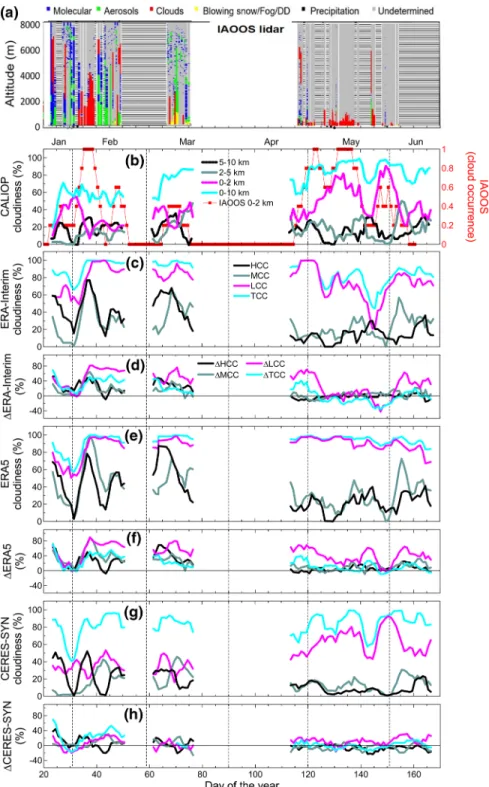
The IAOOS lidar observations show a high occurrence of clouds (Figures 3a and 3b), in particular between days 30 and 40 (early February) that are associated with storm events seen in Figure 2a. More stable mete-orological conditions were reached during spring, with a persistent layer of low-level clouds. These were mostly water clouds as characterized by strong backscattering and attenuation (Di Biagio et al., 2018) ob-served by IAOOS during May (days 120–150). The dominance of low-level clouds in spring in this region is confirmed by CALIOP observations (Figure 3b); in this dataset, clouds below 2 km represent between 40% and 100% of the total cloud cover between days 120 and 170. Examining the CALIOP observations at larger scales (not shown) suggests that low-level clouds in spring occur frequently over the entire Arctic Ocean, which may be linked to Bering and Siberian air inflows (Di Biagio et al., 2018).
Figure 3 also shows that some differences exist between the IAOOS and CALIOP cloud observations, par-ticularly in winter. This is probably due to the different temporal and spatial sampling between the two data-sets: IAOOS are local scale observations over 10-min averages every 4 h, whereas CALIOP data are averages over ±2° around the IAOOS position over several overpasses that are hours apart. Moreover, the IAOOS lidar is looking from the surface, not detecting clouds above low clouds when they are present (mostly water clouds in spring as previously mentioned). Whereas, CALIOP measures the entire troposphere using obser-vations from the top of the atmosphere, with exception of some low-level clouds (Blanchard et al., 2014). Compared to CALIOP observations, both ERA-Interim and ERA5 generally overestimates cloud cover at all levels during wintertime over the study region (Figures 3c–3f). This difference in cloud cover was already identified in previous studies over the Arctic Ocean (Zygmuntowska et al., 2012), and in particular during storm periods. On the contrary, both reanalysis products perform well at reproducing the occurrence of medium and high clouds compared to CALIOP during spring, as well as the dominance of LCC during this period, which is present in both the CALIOP and IAOOS datasets. Nonetheless, the exact amount and temporal variations of cloud cover at all levels is somewhat different in ERA-Interim and ERA5 compared to CALIOP and IAOOS, with periods of both underestimation and overestimation of LCC and/or TCC in ERA-Interim and a general overestimation of LCC in ERA5. In particular, it is seen that during May, although good agreement in low cloud cover is observed, most of the time the associated COT remains smaller in ERA-Interim (see Figures 4a and 4b). Indeed, only the mid-May (days 135–142) and June pe-riods show significant liquid water content and higher COT in ERA-Interim (see Figure 4c). Examples of the distribution of the ERA-Interim and ERA5 COT over the analyzed region in three different periods in spring are shown in Figure S3. It is interesting to note from Figure 3 that the TCC is always larger than 50% for reanalysis products, including non-negligible amount of both low and high clouds, also during the clear periods identified in the temperature dataset in Figure 2a in January and February. The COT is however about zero during the winter clear periods in both ERA-Interim and ERA5 and associated to almost zero water, suggesting that very thin clouds contribute to the cloud cover in these periods.
Figure 3. (a) Vertical cross section of the feature classification from IAOOS lidar observations co-located with N-ICE2015 observations (DD indicates Diamond
Dust; white regions correspond to periods with no measurements, while gray parts stands for altitudes where the lidar signal was not exploitable); (b, c, e, and g) vertically resolved cloud occurrence obtained from CALIOP measurements, ERA-Interim and ERA5 reanalysis datasets, and CERES-SYN (from MODIS algorithm), respectively, in the period from January–June 2015 north of Svalbard. For CERES-SYN cloud HCC correspond to the mid-high clouds, MCC to the mid-low clouds, and LCC to the low clouds classes. Five day running average of IAOOS low clouds (<2 km) occurrence is also shown in panel (b). Panels (d, f, and h) report the differences in cloud occurrence between ERA-Interim, ERA5, CERES-SYN, and CALIOP, respectively. The ΔHCC is (HCC—CALIOP 5–10 km), ΔMCC is (MCC—CALIOP 2–5 km), ΔLCC is (LCC—CALIOP 0–2 km), and ΔTCC is (TCC—CALIOP 0–10 km). The ERA-Interim, ERA5, and CERES-SYN data are within ±0.5° lat/lon from daily N-ICE2015 average position whereas CALIOP is within ±2.0°. Data are shown as 5-days running averages in all plots with the exception of the IAOOS profiles in (a) that are measured at 10-min intervals. CALIOP, Cloud and Aerosol Lidar with Orthogonal Polarization; CERES, Clouds and the Earth's Radiant Energy System; ERA, ECMWF reanalysis; HCC, high cloud cover; IAOOS, Ice-Atmosphere-Arctic Ocean Observing System; LCC, low cloud cover; MCC, middle cloud cover; TCC, total cloud cover.
The CERES-SYN product reproduces the cloud occurrence very well and the repartitioning of low, medium, and high clouds as compared to CALIOP data in the spring to summer time (Figures 3g–3h). However, an overestimation of cloud occurrence at all levels (as well as COT in clear periods) is detected in wintertime compared to CALIOP observations, but a lower cloud cover is usually found compared to reanalysis. Note that the cloud levels are not exactly the same between the different products, and this may lead to some discrepancy. It should be mentioned that previous works have indicated underestimation of CERES cloud occurrence in the Arctic linked with the dominance of thin clouds in this region and the relative high COT threshold values in MODIS cloud mask algorithms (e.g., COT of 0.5 for the MODIS 1621 product for bright surfaces for instance leading to 22% undetected clouds in the Arctic, Chen et al., 2019). This underestima-tion is not apparent in our dataset compared to CALIOP observaunderestima-tions.
As shown in Figure 4c, the CLW and CFW is significantly higher in CERES compared to ERA-Interim, leading to a COT larger than five for CERES most of the time in spring, and much smaller values (frequently
Figure 4. (a) Visible cloud Optical thickness (COT) from ERA-Interim, ERA5, and CERES-SYN and the COT from the
radiative transfer code (RTC). (b) COT for liquid and ice clouds, (c) cloud liquid, and (d) cloud frozen water content (CLW, CFW) for ERA-Interim, ERA5, and CERES-SYN. Data are shown as daily averages. The COT for ERA-Interim and ERA5 is retrieved from Equation 2 assuming a fixed Reff for clouds. CERES, Clouds and the Earth's Radiant Energy System;ERA, ECMWF reanalysis.
below 1) for ERA-Interim. The CLW and CFW for CERES on the contrary are at about 0.5 and 1 kg m−2
almost constantly during winter (as well as the COT), therefore they do not reproduce the alternation of clear and storm periods as instead reproduced in ERA data as the combination of liquid and ice clouds. This results, as previously noted, in an overestimate of the COT in clear periods and an underestimate during storm periods in winter in the CERES dataset. The COT from CERES for April and May is in good agreement with the COT retrieved from the N-ICE2015 radiation measurements using the radiative transfer code simulations. The ERA5 dataset shows larger CLW compared to ERA-Interim (up to 5 times higher) in particular during spring leading to considerably higher COT values than ERA-Interim, values that are in good agreement with CERES and RTC estimates. However, it is interesting to note that the COT agrees be-tween ERA5 and CERES in many times in spring even if the corresponding CLW and CFW are significantly higher in CERES data, suggesting different assumptions in MODIS retrieval compared to Equation 2 used here for ERA COT retrieval. Average values of about 5 are seen in early May (days 124–134) and at the end of May (146–151) but are close to 10 for days 135–142. Average values in June are in better agreement with the total optical depths from ERA-Interim over the atmospheric column, although CERES exhibits smaller values near day 163. The clear-sky episodes on days 143 and 166 are well identified, despite a COT between 1 and 5 is obtained.
3.2. Radiative Fluxes
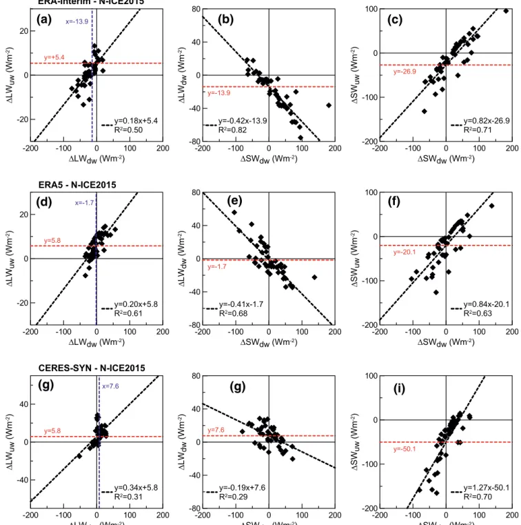
Radiative fluxes measured during N-ICE2015 (Walden et al., 2017) and those from SYN, CERES-EBAF, ERA-Interim and ERA5 are shown in Figure 5. Differences between N-ICE2015 observations and reanalysis/satellite data are illustrated in Figure 6.
Figure 5. (a–f) Temporal evolution of SW and LW downward (dw), upward (uw), and net (dw-uw) irradiance data and (g) total (SW + LW) net irradiance for
N-ICE2015 and co-located ERA-Interim, ERA5, CERES-SYN, and CERES-EBAF datasets. All data are shown as daily averages except CERES-EBAF data that are monthly averages. For the sake of clarity error bars are not shown in the plots. Clear sky episodes (days 143 and 166) are marked by vertical dotted lines. Data interruptions occurred in different periods due to N-ICE2015 measurement gaps or due to data quality. CERES, Clouds and the Earth's Radiant Energy System; ERA, ECMWF reanalysis; LW, longwave; N-ICE2015, Norwegian young sea ICE cruise; SW, shortwave.
3.2.1. Winter Longwave Radiation
In winter, as discussed by Graham et al. (2017a) and Walden et al. (2017), and in agreement with earli-er SHEBA data (Shupe & Intriearli-eri, 2004; Stramler et al., 2011), longwave radiation switches between two states: one with a near neutral LW net budget (LWnet ∼0 Wm−2) namely the “opaquely cloudy state” (storm
periods), and another with a large negative (upward) net longwave radiative flux LWnet of ‒40 to ‒60 Wm−2
namely the “radiatively clear state.” These two states correspond to the warm and cold winter tempera-ture cases shown in Figure 2a. As described by Graham et al. (2019), ERA-Interim and ERA5 capture the “opaquely cloudy” and the “radiatively clear” states and their transition during N-ICE2015, as shown in LW fields (Figures 5a–5c). However, clear states are associated with a high positive surface temperature bias, resulting in an overestimation of LWuw. A negative bias is observed for both LWuw and LWdw radiation
com-ponents during the “opaquely cloudy” storm periods, possibly due to the fact that the enhanced cloudiness compared to observations (Figures 3c–3d), is not capable to fully compensate for lower CLW and CFW in the ERA-Interim as previously identified (Lenaerts et al., 2017). The ERA5 LWdw dataset is also biased high
in clear sky period in early February (Graham et al., 2019). As a result, the total net radiation in winter from ERA-Interim and ERA5 is in agreement with N-ICE2015 during storms and periods of high cloudiness. However, the net radiation is significantly underestimated during clear periods in particular for ERA-Inter-im, leading to a net surface cooling from that is, about 25–30 W m−2 larger than the observations on daily
time scales. The negative bias is lower for ERA5, but particularly in early February this reflects a larger compensation of downward and upward LW biases.
The CERES-SYN data reproduce the transition between clear and cloudy periods in winter in LWdw and
LWuw data, but both components are positively biased during clear phases due to the temperature bias
and the overestimate of COT during clear-sky periods in the CERES product (Figure 4a). The LWdw is also
strongly biased low (down to 40 W m−2) during storm periods because of the underestimation of COT as Figure 6. Differences between ERA-Interim, ERA5, and CERES-SYN daily and CERES-EBAF monthly LW, SW, and net radiation data from N-ICE2015
observations. Horizontal dotted lines represent constant values of ±25 Wm−2. CERES, Clouds and the Earth's Radiant Energy System; ERA, ECMWF reanalysis; LW, longwave; N-ICE2015, Norwegian young sea ICE cruise; SW, shortwave.
shown in Figure 4a. As a consequence, the winter transition between clear and cloudy periods is marked by a shift from positive bias up to about 40 W m−2 during clear periods to negative bias down to 30 W m−2
during storm phases in the LWnet radiation.
3.2.2. Spring Longwave and Shortwave Radiation
The situation changes in spring when cloudiness is dominated by low clouds and local scale forcings as SW radiation is now contributing significantly to the radiative budget. Also, the surface albedo changes as snow melt begins, which affects SW radiation. During spring, there were two short episodes of clear skies on days 143 and 166, corresponding to local minima of net LW radiation. The second episode is outside of the period of IAOOS observations, but the first one corresponds to a transition between low-level dense water clouds to mid-level extended ice clouds (Figure 3b). This decrease is also seen in the larger-scale cloud fractions from CALIOP, ERA-Interim and CERES-SYN data (Figures 3b–3g) but not in the ERA5 dataset (Figure 3e). In spring, LWuw radiation from ERA-Interim and ERA5 is in good agreement with observations (Figures 5a–
5c), as expected from surface temperature agreement between reanalysis and observations. A systematic and strong bias is seen in LWnet cooling for ERA-Interim, which originates from a low bias in the downward
LW radiation. Thus, the net LW cooling in ERA-Interim can reach -80 Wm−2 on daily time scales and can,
at times, provide 60 W m−2 more cooling than measured during N-ICE2015. This might be due to a low bias
in the cloud water content and not to the cloud fraction, which is mostly over 60% in May (Figures 3c–3d) except during the clear sky event on day 143. In contrast, better agreement in both upward and downward components and the net LW radiation is found for the ERA5 and the CERES-SYN datasets (within ±25 W m−2) due to the better reproduction of both surface temperature and cloud properties compared to
obser-vations in spring. However, we note a systematic negative bias in LWnet for ERA5 in spring, particularly in
June, and a positive bias in both LWdw and LWnet in ERA5 for day 143 because of an overestimate the COT
during the clear sky day, as shown in Figure 4a. The CERES-SYN reproduces well the LWnet throughout
springtime, but we evidence a compensation between a slight positive bias for LWuw in CERES-SYN before
day 140 because of a slight temperature bias and a slight negative bias of LWdw.
Figures 5d–5f shows that the two clear-sky events on days 143 and 166 lead to peaks in the SW radiation in the observations. The duration in particular of the first event seems to be much longer in the ERA-Interim dataset, extending from day 143–152, when the cloud optical thickness remains close to zero (Figure 4a). The temporal resolution of the clear-sky events is better captured by ERA5 and CERES-SYN. Good overall agreement between ERA-Interim, ERA5, and the N-ICE2015 data is observed for both the upward and downward SW radiation before day 145, when we can also assume N-ICE2015 point measurements repre-sentative of the ±0.5° grid averages because of the homogeneity of sea ice and albedo over the region, as discussed in Section 3.1.2. For CERES-SYN, the SWdw component is in good agreement with observations
before day 145, whereas the SWuw is systematically biased low by up to 50 Wm−2 on daily scale.
After day 145, when sea ice melting begins, the N-ICE2015 point data cannot be used anymore as reference, and in fact we observe a significant deviation of both satellite and reanalysis data from surface observa-tions, in particular in the SWuw component. The SWuw is systematically lower (by more than 100 Wm−2)
for CERES-SYN between days 145 and 155 compared to reanalysis, while the three data sets agree within their uncertainties afterward, but being always lower than N-ICE2015 point data. The SWdw component is
systematically higher for ERA-Interim in the aftermath of the clear sky period between days 144 and 152 compared to ERA5 and CERES-SYN, as anticipated because of the low COT in this dataset. Thereafter the SWdw component is in good agreement between ERA-Interim and ERA5 during June, but higher in
CERES-SYN between about days 155–160 because a lower COT, as also identified as negative bias in LWdw data. To
note that the sharp peak in ΔSWdw and ΔSWuw seen in all data for day 158 and reaching about 220 Wm−2 in
CERES-SYN and 140 to 180 Wm−2 in ERA5 and ERA-Interim is also the result of only partial N-ICE2015
observations during that day, therefore biasing the observational reference data.
Surface heating due to positive SWnet is in good agreement between reanalysis and observations before day
145, while the SWnet is larger in CERES-SYN. The CERES-SYN shortwave heating is much larger also
com-pared to reanalysis products after day 145, reflecting the differences in surface albedo as shown earlier. The SW surface net heating can be as large as 120 W m−2 on daily time scales for ERA-Interim and ERA5 with
and an absolute peak of 96 W m−2 in the observational dataset. The CERES-SYN surface heating may reach
about 200 W m−2 on a daily basis.
3.2.3. Winter to Spring Net Radiation Budget
The total net radiation (Figure 5g) shows a steady evolution of the N-ICE2015 net radiation budget over the first 6 months of the year, from a minimum of -60 W m−2 in winter to a maximum of 50 W m−2 at the end of
spring. Results from ERA-Interim and ERA5 for total radiation are in agreement with observations within ±25 Wm−2 from the end of winter through the end of May. In June, the differences between ERA datasets
and N-ICE2015 reach up to 70 W m−2 on daily time scales due to the strong overestimate of the SW net
radi-ation in link with the spatial representativeness of the albedo in N-ICE2015 observradi-ations. The CERES-SYN data overestimate the total net radiation in the whole winter to springtime period with differences below 50 W m−2 before mid-May and up to 120 W m−2 afterward compared to N-ICE2015 point observations and
up to 80 W m−2 compared to reanalysis data. The only exception is the negative bias of total net radiation
during winter cloudy period around days 35–40 and day 47.
3.2.4. Springtime Transition From Sea Ice to Sea Ice Melting Conditions
To have a more detailed view on the variability of the fluxes and the representativeness of average values for evolving surface state and ice conditions, we have reported in Figures 7 and 8 the histograms of SW and LW fluxes derived for three 5-days periods, regularly spaced from end of April to early June, from reanal-ysis data and N-ICE2015 observations. These periods correspond to days 115–120, 135–140, and 155–160, representative of homogeneous sea ice conditions over the studied region (115–120, 135–140) and the sea ice melting period (155–160). The figures illustrate that while the distribution of LW radiation is basically monomodal around average values for all datasets, the distribution of SW data is more flat because of the stronger variation of SW radiation in link with solar zenith angle, clouds, and surface albedo. Therefore, average values for SW radiation are affected by larger uncertainties than LW data to represent variation in irradiance levels over daily scales. However, this does not affect the identified biases. For instance, during period 115–120 both SWdw, SWuw, and LWdw are biased low in ERA-Interim, and this is the result of albedo
and COT underestimation, as illustrated both as histograms in the investigated regions/time period in Fig-ures S2 and S3 of the supporting information, while the bias is lower in ERA5 data compared to observa-tions. The period 135–140 is affected by a stronger underestimation of COT for liquid clouds by ERA-Inter-im data compared to ERA5, as evidenced by both histograms (Figure S3) and daily averages (Figure 4), and this induces a strong negative bias in LW radiation and a positive bias in the SW field, while surface albedo differences play a minor role. For the days 155–160, when sea ice melting is taking place over the analyzed area, the reanalysis products show differences from point SW N-ICE2015 data, and a lower bias compared to observations is obtained for LWdw and LWnet from reanalysis.
3.2.5. Monthly Means
Table 1 summarizes all the monthly means from N-ICE2015, ERA-Interim, ERA5, and CERES-EBAF/SYN data and their differences for the months of February, May, and June. Analysis of monthly means allows quantification of significant biases at longer time scales. The N-ICE2015 observations are in good agree-ment with the SHEBA results (Graham et al., 2017a).
To compare the monthly CERES-EBAF (and ERA-Interim/ERA5) and N-ICE2015 observations, we report SW, LW, and net radiation differences (ΔSW, ΔLW, and Δnet, respectively) and their downward and upward components in Figure 6 also for monthly CERES data.
During winter, the CERES-EBAF total net radiation is about 10 W m−2 lower (in absolute value) than
obser-vations from N-ICE2015. This is due to the upward and downward fluxes exceeding obserobser-vations because of warmer surface temperatures, and COT that are too large during clear periods, as in the CERES-SYN data. As seen in Figures 6c and 6f, the retrieved CERES-EBAF (and ERA-Interim) net SW and LW fluxes show opposite biases of about 25–30 W m−2 with respect to observations in May, in contrast to CERES-SYN that is,
biased only in the SW component by 45 W m−2 over the monthly mean, and ERA5 that shows opposite but
much lower biases (of the order of 10 W m−2 or less) in SW and LW net fluxes. The CERES-EBAF LW bias
is again possibly due to a warm surface temperature bias, a bias that is not detected in the daily SYN data, which might possibly be the result of flux adjustments in the EBAF retrieval. The SW bias in EBAF data
is due to the underestimation of the surface albedo. However, the albedo from the EBAF data is closer to observations than that for the SYN data, so the net SW bias is lower for EBAF than for SYN. The LWnet from
CERES-EBAF is comparable to ERA-Interim in May but they are both biased for different reasons: surface temperature is causing the bias in CERES-EBAF, whereas cloud properties are mostly biasing ERA-Interim (as for example in May, during the cloud biased periods as previously discussed). This bias appears to be maintained in June in CERES-EBAF (in contrast to CERES-SYN) in LWuw data, combined with a possible
bias in cloud properties although much reduced in the analyses.
Similar biases are observed in the SW budget from the end of April through May (prior to the clear skies on day 143) but are of opposite sign. From the end of May and throughout June, SWnet biases increase in
ERA-Interim and ERA5 starting around day 145 (25 May) (SWnet being between 30 and 80 Wm−2 higher
than N-ICE2015), which means a significantly larger surface heating linked with sea ice melting in the
Figure 7. Histograms showing the relative occurrence of the SW downward, upward, and total net radiation measured during N-ICE2015 for the three
different 5-days selected periods and retrieved from ERA-Interim and ERA5 data over the ±0.5° region around N-ICE2015 position. The three periods correspond to the day of the year (DOY) intervals 115–120 (25th to 30th April), 135–140 (15th to 20th May), and 155–160 (4th–9th June). Averages and standard deviation of the radiation components over the five days intervals are reported in each plot (units are Wm−2). ERA, ECMWF reanalysis; N-ICE2015, Norwegian young sea ICE 2015.