HAL Id: insu-01649741
https://hal-insu.archives-ouvertes.fr/insu-01649741
Submitted on 2 Dec 2020HAL is a multi-disciplinary open access archive for the deposit and dissemination of sci-entific research documents, whether they are pub-lished or not. The documents may come from teaching and research institutions in France or abroad, or from public or private research centers.
L’archive ouverte pluridisciplinaire HAL, est destinée au dépôt et à la diffusion de documents scientifiques de niveau recherche, publiés ou non, émanant des établissements d’enseignement et de recherche français ou étrangers, des laboratoires publics ou privés.
Detecting recovery of the stratospheric ozone layer
Martyn Chipperfield, Slimane Bekki, Sandip Dhomse, Neil R. P. Harris, Birgit
Hassler, Ryan Hossaini, Wolfgang Steinbrecht, Rémi Thiéblemont, Mark
Weber
To cite this version:
Martyn Chipperfield, Slimane Bekki, Sandip Dhomse, Neil R. P. Harris, Birgit Hassler, et al.. De-tecting recovery of the stratospheric ozone layer. Nature, Nature Publishing Group, 2017, 549 (7671), pp.211 - 218. �10.1038/nature23681�. �insu-01649741�
1
Detecting Recovery of the Stratospheric Ozone Layer
Martyn P. Chipperfield1,2, Slimane Bekki3, Sandip Dhomse1, Neil R.P. Harris4, Birgit Hassler5, Ryan Hossaini6, Wolfgang Steinbrecht7, Rémi Thiéblemont3 and Mark Weber8
1. School of Earth and Environment, University of Leeds, UK.
5
2. National Centre for Earth Observation, University of Leeds, U.K. 3. LATMOS-IPSL, Paris, France.
4. Centre for Atmospheric Informatics and Emissions Technology, Cranfield University, UK. 5. Bodeker Scientific, New Zealand.
6. Lancaster Environment Centre, Lancaster University, UK.
10
7. Deutscher Wetterdienst, Hohenpeissenberg, Germany.
8. Institute of Environmental Physics, University of Bremen, Germany.
Revised version 2 July 28, 2017
15
As a result of the 1987 Montreal Protocol and its amendments, the atmospheric loading of anthropogenic ozone-depleting substances is decreasing. Accordingly, recovery of the stratospheric ozone layer is expected. However, short data records and atmospheric variability confound the search for early signs of recovery. Moreover, climate change is masking ozone recovery from ozone-depleting
20
substances in some regions and will increasingly affect the extent of recovery. Here we discuss the nature and timescales of ozone recovery, and explore the extent to which it can be currently detected in different atmospheric regions.
Depletion of the stratospheric ozone layer has been one of the most prominent environmental issues of the past 40 years. The layer prevents biologically damaging solar
25
ultraviolet (UV) radiation (wavelengths below about 300 nm) from reaching the surface and was thus a key factor in creating the conditions for the evolution of life on earth1. Ozone is also an efficient absorber of terrestrial infra-red radiation and therefore a ‘greenhouse’ gas, albeit one that is produced in the atmosphere rather than emitted at the surface. In recent years it has become clear that there is a strong coupling between stratospheric ozone and
30
climate change.
Serious concern over ozone depletion started in the 1970s when it was realised that the break-down of man-made compounds such as chlorofluorocarbons (CFCs) in the middle stratosphere would release chlorine atoms which could catalytically destroy ozone2,3. Research activity increased greatly following the discovery in 1985 of large and unexpected
35
depletion in the Antarctic lower stratosphere during spring4, the so-called Antarctic ozone hole. This depletion was caused by increasing levels of chlorine and bromine in the atmosphere but, crucially, also involved the conversion of stable chlorine reservoir species into active ozone-destroying forms on the surface of polar stratospheric clouds which form in winter and spring5. Atmospheric scientists failed to predict the ozone hole in advance as the
40
models used to forecast the evolution of the ozone layer did not include such processes6. By the time of the discovery of the Antarctic ozone hole the process for international protection of ozone layer had already been initiated and the framework for its implementation
2
set up by the signing of the Vienna Convention in 1985. The Montreal Protocol on Substances which Deplete the Ozone Layer was signed in September 1987 and ratified by
45
January 1989. The protocol, with its 30th anniversary this year, was a major achievement in terms of global environmental protection although it initially placed only modest limits on the production and consumption of major ozone-depleting substances (ODSs) such as CFCs and bromine-containing halons. Importantly, the protocol allowed for further strengthening through later amendments and adjustments, and over time these revisions have led to an
50
almost complete ban on major classes of ODSs including CFCs, replacement hydrochlorofluorocarbons (HCFCs) and related compounds such as methyl chloroform and carbon tetrachloride. These compounds have atmospheric lifetimes of the order of 10-100 years7, and so the response of the atmospheric chlorine and bromine loading to changes in emissions is slow. Nevertheless, observations show5 that the abundance of these gases in
55
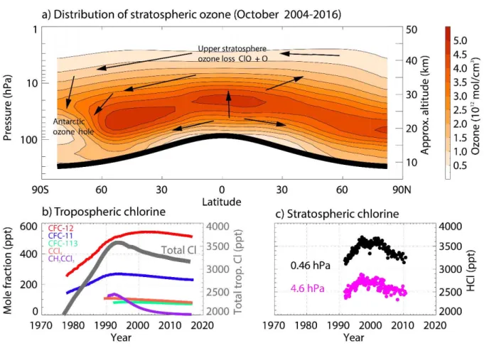
the lower atmosphere is largely responding to the Montreal Protocol limits as expected and most major ODSs are decreasing (Figure 1). The sum of tropospheric chlorine peaked in 1993 and the sum of tropospheric bromine peaked a few years later in 1997. The stratospheric abundance of chlorine (which largely resides as HCl in the upper stratosphere8) and bromine, derived from these ODSs, followed these tropospheric
60
variations but with a delay of ~3 to 7 years (depending on the region) due to the slow timescale for transport and degradation of ODSs through the stratosphere9. Accordingly, we expect stratospheric ozone depletion due to chlorine and bromine to follow this behaviour of increasing depletion through the late 1990s, followed by a turn-around and slow ‘recovery’. Unfortunately, variability in other factors affecting ozone, such as stratospheric dynamics
65
(i.e. wind, temperature), aerosol loading, and solar irradiance, all complicate this simple picture and mask the small signal of ozone recovery from ODSs – expected to be around a few percent per decade globally. An important question is therefore to what degree and where can we detect ozone recovery. A further important question is the ultimate extent to which the ozone layer will recover, given the increasing impact of climate change on
70
atmospheric structure and composition. In this perspective, we analyse what observations and models can already tell us about the current status of recovery is and where ozone is heading. We show that ozone recovery is proceeding consistent with our understanding and argue that it should not be seen as a single detectable event, but rather a slow direction of travel for which the evidence will become gradually clearer as our data records increase.
75
Recovery of the Ozone Layer
Although the concept of an ‘ozone layer on the mend’ may appear simple, discussions on this topic within the atmospheric science community are often heated and become very nuanced. So, why is detecting the recovery of the stratospheric ozone layer a tricky subject?
80
Can’t we just define recovery as when ozone levels return to their former values before significant ozone depletion occurred? At first that appears conceptually trivial, but complications immediately arise when we consider that the rest of the atmosphere is also changing. The continuing rise in CO2 is altering the physical structure of the atmosphere: the tropopause is rising so the stratosphere is getting thinner; its temperature structure is
85
changing, and the Brewer-Dobson Circulation in which air is transported into and through the stratosphere (Figure 1) may accelerate in the future10. As a result, there may be stronger upwelling in the tropics and faster descent over the middle latitudes and polar regions. Because ozone abundance increases with altitude in the lower stratosphere (where most of
3
the ozone resides), this would lead to less ozone in the tropics and more ozone at higher
90
latitudes. Cooling in the upper stratosphere is already increasing ozone in that region by slowing gas-phase ozone destruction cycles11,12. All these changes are driven fundamentally by increasing greenhouse gases (GHGs), especially CO2. At the same time, N2O and CH4 are also currently increasing, with CH4 in particular very sensitive to variations in emissions from its natural and anthropogenic sources13. The balance between the various catalytic
95
cycles which result from ODS, CH4 and N2O degradation and drive ozone loss will therefore change as well. What is clear is that the chemistry and dynamics of the stratosphere will have changed sufficiently that recovery to ozone levels prior to ozone depletion is not a sensible concept. The picture is complicated further when we consider how recovery occurs in different parts of the atmosphere or in different seasons.
100
If the atmosphere is not returning to its former state, then should we not look to changes in surface UVB radiation (or even the consequences) as the best measure for recovery? After all, the motivation for the Montreal Protocol was to avoid the risk of health and other impacts of increased UVB. However, possible changes in non-stratospheric factors such as tropospheric ozone, clouds, aerosols and the earth’s albedo, coupled with their large
105
variability, all make it hard to draw meaningful conclusions about recovery of surface UVB14. It is a more complex picture even than for ozone.
From a regulatory point of view, as control of production and consumption is the tool that policy-makers can employ, the success of the Montreal Protocol is judged primarily by the changes in atmospheric ODS concentrations. From this perspective, the Montreal Protocol is
110
already undoubtedly a success; ODS levels are decreasing15 with expected benefits for ozone and UVB radiation and also for climate. However, the impact of these ODS declines on ozone levels has proved much harder to detect.
Definitions of ozone recovery have tended to be based on the concept of a state or stage being reached. Since recovery is often defined with respect to the effect of ODSs (the key
115
factor in the Montreal Protocol), each stage requires a clear attribution of ozone changes to the decline and ultimately return of ODSs to their pre-industrial levels16. The following stages (or fingerprints) of recovery have been defined16: 1) a significant slowing down of stratospheric ozone decline; then 2) the onset of a significant increase; and finally 3) the full recovery of ozone from ODSs, when ozone is no longer significantly affected by them.
120
However, it is more beneficial to think of recovery as the direction of travel rather than the destination. Indeed, full recovery does not necessarily imply a return of stratospheric ozone to pre-1980 levels because the influence of other factors, notably increasing GHG levels, is growing. The ODS levels in the atmosphere are clearly decreasing (Figure 1) and the first stage (or ‘fingerprint’) of the ozone response, the end of the ozone decline, has been
125
observed5,17. However, it has been difficult to establish the occurrence of the next stage, i.e. a general upward trend in ozone due to declining ODSs. This may be surprising, since ODS levels have now been in decline for 15 to 20 years. However, due to the long atmospheric lifetimes of ODSs (typically many decades7), this decline is about three times slower than their rapid increase before the Montreal Protocol came into effect. Back then, it took 10 to 15
130
years to clearly detect the significant decrease in global ozone. Everything else being equal, we might expect 30 to 40 years before detecting a significant upward trend in global ozone due to declining ODS levels becomes possible18.
Diagnosing Ozone Recovery from Current Observations
4
Regular stratospheric ozone observations started with ground-based Dobson spectrophotometers in the mid-1920s19,20. Continuous measurements from space started in 1978 with the Solar Backscatter UltraViolet (SBUV) instrument21 and so global ozone observations now span a time period of nearly forty years (see Figure 2). This includes about 20 years of observations after the global stratospheric ODS peak around 1997 (or 16
140
years after the later ODS peak in polar regions9). The length of the observable recovery period thus covers about two decades which is short to identify uniquely ODS-related recovery among other sources of variability that operate on multi annual or decadal timescales. However, given the importance of this topic there have been many studies which have investigated observationally based ozone trends over this period22–28.
145
Satellite and ground-based data revealed a dramatic decline in the total ozone column (i.e. the total number of ozone molecules in the whole depth of the atmosphere, per unit area) of about 3%/decade until the mid-1990s, caused by ODS increases (Figure 2). In the NH, the lowest annual mean total ozone columns occurred in 1992, resulting from enhanced ozone destruction linked to heterogeneous chemistry on volcanic aerosols and transport
150
changes29–31, after the major volcanic eruption of Mt Pinatubo in 1991, a few years before the peak in stratospheric ODS. In the late 1990s, annual mean total ozone increased rapidly, faster than expected from the slow decrease in ODS. This is related to variability in atmospheric dynamics, notably for ozone transport, exemplified by the Brewer-Dobson circulation32,33. All long observational time series show such decadal variability (e.g. the
155
record at Arosa Switzerland since 192534).
Since 2000, stratospheric ODS levels have been decreasing slowly (at only 1/3 of the rate of the previous ODS increase), and extratropical total ozone has levelled off. Figure 2 also shows results of a multiple linear regression (MLR, see Supplementary Information) with independent linear trends before and after the ODS peak in 1996 (2000 for the polar
160
regions9) applied to annual or September mean total ozone. The MLR approach is used here to linearly decompose the ozone variability into components of a long-term trend and shorter term variability. The regression accounts for well-established sources of shorter term ozone variability (solar variations, stratospheric aerosols, variations in the Brewer-Dobson circulation, modes of climate variability such as the quasi-biennial oscillation (QBO) and El
165
Nino Southern Oscillation). In the tropics and at mid-latitudes, linear trends after 1997 are generally small and not statistically significant. In the tropics, observed total ozone has not changed much at all over the entire time period since 1979. The only region with a possibly significant positive trend in total ozone in the last decade is the Antarctic in September (the month when the ozone hole reaches its maximum areal extent), see Figure 2 or results
170
from35–38; however, results are sufficiently sensitive to uncertainties in the MLR and to the inclusion or not of a specific year in the time series, that formal identification of Antarctic ozone recovery remains uncertain (see37 and Figure S1 in Supplementary Information). Antarctic October time series shows no significant trend, nor does the Arctic in February and March (not shown).
175
The interannual variability of ozone is largest in the lower stratosphere (which dominates the behaviour of the total column). It is much smaller in the upper stratosphere where the end of the ozone decline (the first sign of ozone recovery) was first detected17. Vertically resolved ozone measurements (from multiple satellite and ground-based instruments) have now reported a possible signal of the next stage of recovery in the upper stratosphere, with ozone
180
5
unclear39. Figure 3 shows the corresponding updated ozone time series at 40 km (2 hPa). Nearly all the different observational datasets closely follow the inverted curve of stratospheric chlorine loading. However, model results show that both ODS and greenhouse gases have contributed equally to the recent upper stratospheric increase5.
185
Key issues in the detection of ozone increases from observations are the availability of several independent long-term records (to quantify uncertainty in the data) and the uncertainties of the trend estimates. Optimally, the total uncertainty should include any uncertainties based on: 1) the measurement technique40, 2) data sampling41,42, 3) the uncertainties introduced by the regression, 4) uncertainties from data preparation, especially
190
merging data from different satellites to create a full time series, and 5) differences of trends from different observation systems. While the first two sources of uncertainty are relatively well understood41, the last three have only started to be addressed in recent years. Consistent multi-decadal, vertically resolved ozone measurements from a single instrument are available only from a few sparse ground-based stations43–45. Satellite measurements do
195
provide global coverage, but no single satellite instrument spans the several decades necessary for a robust analysis of both the ozone decline and the expected subsequent increase. Therefore, measurements from different satellite instruments are being combined46–51 but individual satellite instrument characteristics (offsets and drifts) are difficult
to determine52–55. At this point robust records with comprehensive uncertainties have not
200
been achieved and a full uncertainty calculation for vertically resolved ozone trends is still missing (see39,5).
Diagnosing Ozone Recovery from Atmospheric Models
Attribution of ozone trends to specific factors (e.g. evolution of ODS levels) requires the use
205
of atmospheric chemical-dynamical models. These models, although they are by no means perfect and often show significant differences compared to observations and other models, encapsulate our best understanding of the fundamental physics and chemistry that control ozone and its variations. Those most suited for diagnosing ozone recovery are chemical transport models (CTMs) and chemistry-climate models (CCMs). Both include relevant
210
internal and external drivers, especially changing concentrations of ODSs, variations in solar forcing, effects of volcanic eruptions, and changing surface conditions. CTMs are well suited to comparisons with specific observations because dynamics (wind and temperature fields) are prescribed from meteorological re-analyses such as ERA-Interim56 or MERRA57, thus
ignoring feedbacks of chemistry on temperature and dynamics via radiatively driven heating.
215
CCMs normally calculate their own “random” realizations of meteorology, including the feedbacks of changing trace gases on temperature and transport, although they can be nudged to follow prescribed meteorology and therefore perform like a CTM36.
In contrast to observations, models allow us to compare various scenarios with different assumptions of factors affecting ozone. Using different model runs, in combination with
220
observed time series, allows the attribution of ozone changes and thus the diagnosis of ozone recovery without relying on an MLR (as in Figure 2).
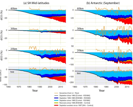
We can use CTM simulations to quantify the expected ozone change in different regions due to separate forcings in the past, notably ODS changes. Figure 4 presents such results from the TOMCAT CTM58 which quantify ozone depletion since 1960, when anthropogenic ODS
225
6
Supplementary Information). The past accumulating emissions of ODSs between 1960
and 1980 contribute more to ozone depletion than the emissions after 1980 (for which the signal only appears in the stratosphere a few years later), illustrating the difference in taking these two baselines as a reference. In any case, the model-predicted signal of recovery from
230
ODS (light green shaded region following peak ODSs in 1995) has clearly only reached a small fraction of this past depletion by 2015. Also shown in Figure 4 is the estimated impact of dynamical variability, mainly through transport, on ozone (orange line). This impact is larger in the lower stratosphere and thus it is important for the total column, since ozone density is generally largest at the higher pressures of the lower stratosphere. The resulting
235
year-to-year variations are clearly larger than the predicted signal in recovery.
Shepherd et al.59 compared column ozone observations with simulations from a CCM nudged with ERA-Interim reanalyses. The difference between a run with 1980 ODS levels and a run with realistically changing ODS indicates that global ozone columns should already have benefited from declining ODS levels. The model results in Figure 4 confirm the
240
findings of Shepherd et al. that by 2010 ODS-related midlatitude column ozone loss had already declined by 10% since the peak ODS loading in the late 1990s. Shepherd et al. also noted that tropospheric ozone increases may have compensated for ozone depletion in the tropical lower stratosphere, explaining the lack of long-term column trend there (Figure 2). As the largest impact of ODSs occurs in the springtime Antarctic lower stratosphere4, it is
245
reasonable to suppose that this may be the region with the earliest and/or clearest signs of ozone recovery17,60,61. Solomon et al.36 analysed Antarctic September column ozone observations through 2014 and found signs of recovery since 2000, at 90% confidence. They did not include the year 2002, with unusual polar vortex behaviour and small ozone loss62–64, in their analysis (see also Figure 2d). Their nudged CCM simulations indicate that
250
about one half of the ozone increase observed in September over the period 2000 to 2014 could be attributed to declining ODS. They attributed the other 50% of the increase to transport changes and the very large ozone holes of 2011 and 2015 to additional chemical losses triggered by aerosol enhancements from relatively small volcanic eruptions in Chile65. However, considerable uncertainties pertain to the simulated effects of transport and aerosol
255
changes. It cannot be ruled out that both have contributed a larger fraction to the observed ozone increase from 2000 to 2014, implying a small impact of decreasing ODS over the period.
Separating small ozone changes due to slowly decreasing ODS (less than a few percent per decade) from large dynamical (transport and temperature) related variations is difficult. This
260
is shown in Figure S2 in the Supplementary Information, which compares the different TOMCAT simulations shown in Figure 4. All time series show large similar inter-annual variations, up to ±10 DU. These are mostly due to meteorological variability, and are not seen with repeating 1980 meteorological conditions every year. The recovery signal due to declining ODS does not exceed +6 DU at mid-latitudes, which is much smaller than the large
265
year-to-year variations. The largest modelled recovery signal is in the Antarctic in September at over 20 DU. Figure S2 also shows that the model captures the large Arctic ozone depletion observed in March 201166,67. This large depletion was caused by exceptionally persistent cold stratospheric conditions and is consistent with our understanding of stratospheric ozone and is within the range of variability expected in the Arctic. Importantly, it
270
does not, therefore, undermine our expectation of long-term ozone recovery as ODS decline. A similar argument applies to the large Antarctic depletion of 201565.
7
In the upper stratosphere ozone concentrations are increased by GHG-induced cooling. The increases of observed ozone in the upper stratosphere at northern mid-latitudes after 2000 discussed above5,39 are of the same magnitude as those calculated by CCM simulations68,
275
giving some confidence in both observations and simulations. Comparison of these different simulations shows that declining ODS and stratospheric cooling have contributed about equally to the observed increase of ozone in the upper stratosphere since 2000; neither factor alone is sufficient to explain the observations. WMO/UNEP5 therefore concluded that declining ODS play a role, and that the signal of ozone recovery from ODS is seen in the
280
upper stratosphere.
The TOMCAT CTM simulations in Figure 4 (and Figure S2) clearly reiterate that the main obstacle to detecting and estimating the small ozone recovery from ODS for the 2000-2015 period is the large year-to-year variations, mostly of dynamical origin. The most common approach to account for this high frequency variability in trend analysis is the MLR, although
285
some of its assumptions may be questioned. In order to test the linear decomposition of ozone variability into independent contributions from different factors and increase the level of confidence in the MLR results, we carry out a trend analysis of observational and model time series. The external factors considered in the MLR (solar, aerosol, detrended heat fluxes (used a proxy for the variations in the Brewer Dobson Circulation), quasi-biennial
290
oscillation (QBO), see also Figure 2) mostly generate high frequency (e.g. year-to-year) variability in ozone. The long-term trend in ozone should be overwhelmingly caused by the decline in ODS and the rise in GHGs. Since the MLR cannot discriminate between these effects, it contains only one trend term.
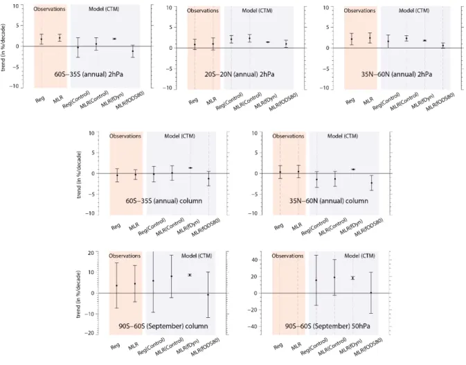
The values of the 2000-2015 ozone trends derived from a simple linear regression (i.e.
295
regression where only a linear trend is fit) and MLR are generally in good agreement for both observations and the model simulations for the tropics, mid-latitudes (NH, SH), and Antarctic (Figure 5). In addition, the MLR trend values for the observations and the control simulation are also consistent within error bars. As expected, the MLR trend representing the effect of declining ODS (‘fixed dynamics’ simulation) is clearly positive in all regions, and most
300
pronounced in the Antarctic. In contrast, the MLR trend attributed to dynamical variability (‘fixed ODS’ simulation) varies strongly from one region to another. For total ozone, the trend is negative at mid-latitudes but null in Antarctica; in the upper stratosphere, it is positive in the tropics and at northern mid-latitudes but negative at southern mid-latitudes. As mentioned before, low frequency natural dynamical variability, e.g. in the Brewer-Dobson
305
circulation, can randomly generate significant trends over 10-15 year periods69. They can mask ozone recovery from ODS. Interestingly, the value of the MLR trend for the control simulation is approximately equal to the sum of those of the ‘fixed dynamics’ and ‘fixed ODS’ simulations, suggesting that the effects of changes in ODS and dynamics are approximately additive and that an attribution analysis based on the simulations is justified70. The
310
uncertainty in the overall trend is dominated by the dynamical variability and large errors bars indicate that the dynamical proxies (QBO, detrended heat flux) in the MLR are not able to account for all the interannual variability. Note that as no ozone-dynamics feedbacks are included in the ‘fixed dynamics’ simulation, our estimation of the declining ODS contribution (inferred from this simulation) is possibly an upper limit, particularly in the upper
315
stratosphere17.
Taken together, Figures 4, 5, and S2 demonstrate how small the expected ozone recovery currently is compared to the confounding interannual dynamical variations. As expected, the
8
most certain signs for a beginning recovery can now be seen in regions where the ozone layer is most sensitive to ODS and the dynamical variability is not too large. These regions
320
are the upper stratosphere5, and, to a lesser extent, the Antarctic in September36, where our model results indicate that statistically significant recovery could be detectable with a suitable observing system. For other regions, variability is too large (e.g. Arctic, extra-tropical lower stratosphere), ODS effects are too small (e.g. tropical stratosphere), negative dynamical trends mask an ODS-driven positive trend (extratropical column ozone) or the
325
observational record is too short or not accurate enough (e.g. tropical lower stratosphere). The discrepancies between observed and simulated total ozone (black and dark blue lines in
Figure S2), notably in the NH midlatitudes in the 1980s and in the Antarctic, indicate that
simulations are subject to additional uncertainties, such as missing processes, uncertain rate constants and incomplete parametrizations, which pose additional challenges for attributing
330
ozone recovery from models.
Expectations for Recovery in the 21st Century
As ODS levels continue to decline throughout this century, the associated ozone recovery signal will become stronger and hence easier to extract, especially with gradually longer data
335
records71. Although ODS changes have been the main driver of ozone evolution throughout most of the stratosphere since the 1970s and will still be important in the future, the influence of increasing GHG concentrations (CO2, N2O, CH4) on global ozone has been growing and will become dominant in the second-half of the century5. Future low frequency variability (trends) in stratospheric ozone will likely be driven by competing effects (e.g. effects of
340
decreasing ODS versus those of increasing GHG) and the complex chemical-dynamical-radiative couplings will not be unravelled easily, again making attribution uncertain.
Our best tools for future ozone projections are 3-D chemistry-climate models, which encompass all relevant knowledge of key processes, but they need to be evaluated against observations and require significant computer resources to run a wide range of scenarios
345
over century timescales. That work is ongoing68,72 but here we show shows some illustrative
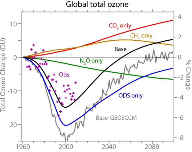
results from a simpler zonal mean latitude-height model (Figure 6). Driven by ODS concentrations declining throughout this century, global ozone is projected to recover its 1980 level by ~2030 and its 1960 level by mid-century for a standard scenario for ODS and GHG emissions (Representative Concentration Pathway (RCP) 6.0, a scenario wherein the
350
combined increase of greenhouse gases produces an increase in radiative forcing of 6 W/m2 by 2100). Note that the projected dates of return to specific historical levels, especially 1960, can vary greatly from model to model. For instance, some models predict a return of global ozone to 1960 level as early as 2030 whereas, according to other models, global ozone barely recovers the 1960 level by the end of century68. Interestingly, the model-projected
355
return of global ozone to historical levels is faster than the return of ODS to their natural levels which is likely to occur towards the end of the century if current control measures of the Montreal Protocol are adhered to in the future. This future accelerated ozone recovery, the so-called ‘super-recovery’, is mainly due to the positive influence of increasing CO2, which cools the upper stratosphere, and therefore reduces the rate of ozone loss, and CH4
360
which influences chlorine partitioning in the upper stratosphere and is a source of odd-hydrogen species which catalytically destroy ozone. In contrast the increase in N2O tends to decrease ozone73 through increased NOx-catalysed loss. Note that the predicted recovery rate for global ozone is strongly sensitive to the assumed future GHG emissions which,
9
unlike ODS emissions, are uncertain, especially in the second half of the century. This, along
365
with model uncertainties, makes model-projected ozone recovery extent and associated return dates to historical levels uncertain.
The combined influence of these drivers (ODS and GHG changes) is predicted to result in a long-term evolution of stratospheric ozone more diverse regionally than would be expected from ODS decline alone. Ozone recovery is projected to be faster in the NH than in the SH5.
370
Although the Antarctic is a region where recovery may be starting to be definitively detectable, it is also where the return of column ozone to 1960 levels is projected to occur relatively late, towards the end of the century, which is about the same time as the return of ODS concentrations to their near-natural 1960 levels68. Although the signal is more difficult to detect74,the return of Arctic ozone to 1960 levels is projected to occur earlier, around
375
2030, which is indicative of the strong influence of rising GHG concentrations75. In contrast to the rest of the globe, the future evolution of tropical ozone column is expected to be essentially driven by changes in GHG levels in the stratosphere and possibly ozone changes in the troposphere. Stratospheric ozone projections in the tropics vary widely with the assumed GHG future emission scenarios of CO2, N2O and CH4. Models predict that the
380
tropical stratospheric partial column ozone may experience either a continued decline (no recovery) with column values lower at the end of the century than the present-day due to enhanced upwelling, or a super recovery with column values higher than the 1960 levels. A future decrease in tropical total (stratosphere + troposphere) column ozone, which models suggest could be a few percent, could have serious consequences as it would increase
385
surface UVB radiation in a region where about 40% of the world population lives and population growth is large. Finally, we note that in some regions future ozone recovery might be affected in the short-term by sporadic volcanic eruptions or by the occurrence of persistently cold Arctic winters such as in 2010/11. They are part of the natural variability and would not impact the long-term ozone recovery76, although there are suggestions that
390
this variability may increase due to climate change, for example, cold winters in the Arctic stratosphere may be getting colder77, though the evidence for this is not conclusive5.
Outlook for the Ozone Layer
Our best understanding indicates that the measures taken to date through the Montreal
395
Protocol have started to remediate ozone depletion and will carry on doing so globally. The measurements and the models are imperfect, but studies have used evidence from both to show there is a consistent picture, in accord with our current understanding, that ozone recovery in the observations is still largely masked by natural variability in most regions but with clear evidence of it in the upper stratosphere and early signs of it in the Antarctic. We
400
can therefore say that we are on track for ozone ‘recovery’. However, we emphasise that ‘recovery’ is not a single event but a continuing journey; as time passes we will have more confidence that it is occurring and a better estimate of its extent. Uncertainty will gradually decrease as measurement records become longer and the growing signal emerges from the underlying natural variability. It is a matter of waiting and ensuring that high quality and
405
consistent observations continue. The quadrennial WMO/UNEP ozone assessment, with the next one due in 2018, is the forum and the milestone for community-wide scientific updates on how far we are on the road to ozone recovery.
10
We need to be vigilant against other factors which may perturb the ozone layer (e.g. extreme dynamical events78,79, volcanic eruptions31,65,80, irregular solar flux variations81, uncontrolled
410
very short-lived halogenated substances82–85, deliberate climate intervention through geoengineering86,87) to ensure that any observed changes are consistent with our understanding and do not change our expectation of long-term recovery. Provided ODS decline continues in the future as mandated by the Montreal Protocol, we will be moving from a stratospheric ozone layer mainly perturbed by anthropogenic chlorine and bromine, to
415
one where the impact of increasing greenhouse gases (CO2, CH4, N2O)88 and associated on-going climate change become more important and dominate after 2050. Safe-guarding the ozone layer in the 2nd half of this century, therefore, will require continued measurements of ozone and ODS as well as of CO2 and the atmospheric temperature structure, but increasingly also measurements of trace gases arising from increased emissions of CH4 and
420
N2O. The fundamental underlying processes are understood and are represented reasonably well in current atmospheric models. Nevertheless, since more factors with competing effects are coming into play, further improvements in these computationally expensive models (and in the machines on which they run) will be necessary, to understand better the measurements, to untangle the more complex interplay of processes controlling
425
stratospheric ozone in the future, and to ascertain that ozone has indeed recovered from anthropogenic ODS by the end of the century. Future knowledge about ozone recovery will require the commissioning and launch of new satellite instruments and the continuation of the ground-based network. In particular, these instruments must measure at a high enough vertical resolution in the lower and mid-stratosphere.
430
Acknowledgements: We are grateful to John Pyle and Paul Newman for helpful comments
on this work. We thank Anja Schmidt for comments on an early version of the manuscript, Eric Fleming for providing Figure 6, and Wuhu Feng for help with TOMCAT. The TOMCAT
435
modelling work was supported by the NERC National Centre for Atmospheric Science (NCAS) and the simulations were performed on the Archer and Leeds ARC/N8 computers. MPC acknowledges support of a Royal Society Wolfson Merit Award. MW acknowledges partial support from the Deutsche Forschungsgemeinschaft (DFG) Research Unit SHARP (Stratospheric Change and its Role for Climate Prediction) and the ESA CCI-Ozone project.
440
RT acknowledges his funding by the LABEX L-IPSL project (grant ANR-10-LABX-18-01). SB and NRPH have been partially supported by the European project StratoClim (603557 under programme FP7-ENV.2013.6.1-2). NRPH also acknowledges support from NERC CAST (NE/I030051/1). We thank the three anonymous reviewers for their comments which helped to improve the manuscript significantly.
445
Author Contribution: MPC initiated the study and recruited the author team. All authors
contributed to the writing of the paper. MPC and SD ran and analysed the TOMCAT simulations. SB, RT and MW performed the MLR studies. RH, MW, WS, SD, RT and MPC produced the figures.
450
11
References
455
1. Wayne, R. P. Chemistry of Atmospheres. (Oxford University Press, 2000).
2. Molina, M. & Rowland, F. Stratospheric sink for chlorofluoromethanes: chlorine atom -catalysed destruction of ozone. Nature 249, 810–812 (1974).
3. Stolarski, R. S. & Cicerone, R. J. Stratospheric Chlorine: a Possible Sink for Ozone.
Can. J. Chem. 52, 1610–1615 (1974). 460
4. Farman, J. C., Gardiner, B. G. & Shanklin, J. D. Large losses of total ozone in Antarctica reveal seasonal ClOx/NOx interaction. Nature 315, 207–210 (1985). 5. World Meteorological Organization (WMO). Scientific Assessment of Ozone
Depletion: 2014, Global Ozone Research and Monitoring Project - Report No. 55.
(2014).
465
6. Solomon, S., Garcia, R. R., Rowland, F. S. & Wuebbles, D. J. On the depletion of Antarctic ozone. Nature 321, 755–758 (1986).
7. SPARC. Lifetimes of Stratospheric Ozone-Depleting Substances, Their
Replacements, and Related Species. (World Climate Research Programme,
WCRP-15/2013, 2013).
470
8. Michelsen, H. A. et al. Stratospheric chlorine partitioning: Constraints from shuttle-borne measurements of [HCl], [ClNO3], and [ClO]. Geophys. Res. Lett. 23, 2361– 2364 (1996).
9. Newman, P. A., Daniel, J. S., Waugh, D. W. & Nash, E. R. A new formulation of equivalent effective stratospheric chlorine (EESC). Atmos. Chem. Phys. 7, 4537–4552
475
(2007).
10. Butchart, N. et al. Chemistry-climate model simulations of twenty-first century stratospheric climate and circulation changes. J. Clim. 23, 5349–5374 (2010). 11. Haigh, J. D. & Pyle, J. A. Ozone perturbation experiments in a two-dimensional
circulation model. Q. J. R. Meteorol. Soc. 108, 551–574 (1982).
480
12. Jonsson, A. I., Fomichev, V. I. & Shepherd, T. G. The effect of nonlinearity in CO2 heating rates on the attribution of stratospheric ozone and temperature changes.
Atmos. Chem. Phys. 9, 8447–8452 (2009).
13. Nisbet, E. G. et al. Rising atmospheric methane : 2007-14 growth and isotopic shift .
Global Biogeochem. Cycles 30, 1356–1370 (2016). 485
14. McKenzie, R. L., Aucamp, P. J., Bais, A. F., Björn, L. O. & Ilyas, M. Changes in biologically-active ultraviolet radiation reaching the Earth’s surface. Photochem.
Photobiol. Sci. 6, 218–231 (2007).
15. Montzka, S. A. et al. Present and future trends in the atmospheric burden of ozone-depleting halogens. Nature 398, 690–694 (1999).
490
16. World Meteorological Organization (WMO). Scientific Assessment of Ozone
Depletion: 2006, Global Ozone Research and Monitoring Project - Report No. 50.
(2007).
17. Newchurch, M. J. et al. Evidence for slowdown in stratospheric ozone loss: First stage of ozone recovery. J. Geophys. Res. 108, 4507 (2003).
495
18. Weatherhead, E. C. et al. Detecting the recovery of total column ozone. J. Geophys.
12
19. Dobson, G. Forty years’ research on atmospheric ozone at Oxford: A history. Appl.
Opt. 7, 387 (1968).
20. Staehelin, J. et al. Total ozone series at Arosa (Switzerland): Homogenization and
500
data comparison. J. Geophys. Res. 103, 5827–5841 (1998).
21. McPeters, R. D., Bhartia, P. K., Haffner, D., Labow, G. J. & Flynn, L. The version 8.6 SBUV ozone data record: An overview. J. Geophys. Res. 118, 8032–8039 (2013). 22. Reinsel, G. C. et al. Trend analysis of total ozone data for turnaround and dynamical
contributions. J. Geophys. Res. 110, D16306 (2005).
505
23. Zanis, P. et al. On the turnaround of stratospheric ozone trends deduced from the reevaluated Umkehr record of Arosa, Switzerland. J. Geophys. Res. 111, D22307 (2006).
24. Dhomse, S., Weber, M., Wohltmann, I., Rex, M. & Burrows, J. P. On the possible causes of recent increases in northern hemispheric total ozone from a statistical
510
analysis of satellite data from 1979 to 2003. Atmos. Chem. Phys. 6, 1165–1180 (2006).
25. Angell, J. K. & Free, M. Ground-based observations of the slowdown in ozone decline and onset of ozone increase. J. Geophys. Res. 114, D07303 (2009).
26. Chehade, W., Weber, M. & Burrows, J. P. Total ozone trends and variability during
515
1979–2012 from merged data sets of various satellites. Atmos. Chem. Phys. 14, 7059–7074 (2014).
27. Nair, P. J. et al. Subtropical and midlatitude ozone trends in the stratosphere: Implications for recovery. J. Geophys. Res. 120, 7247–7257 (2015).
28. Yang, E.-S. et al. Attribution of recovery in lower-stratospheric ozone. J. Geophys.
520
Res. 111, D17309 (2006).
29. Poberaj, C., Staehelin, J. & Brunner, D. Missing Stratospheric Ozone Decrease at Southern Hemisphere Middle Latitudes after Mt. Pinatubo: A Dynamical Perspective.
J. Atmos. Sci. 68, 1922–1945 (2011).
30. Aquila, V., Oman, L. D., Stolarski, R., Douglass, A. R. & Newman, P. A. The
525
Response of Ozone and Nitrogen Dioxide to the Eruption of Mt. Pinatubo at Southern and Northern Midlatitudes. J. Atmos. Sci. 70, 894–900 (2013).
31. Dhomse, S. S. et al. Revisiting the hemispheric asymmetry in mid-latitude ozone changes following the Mount Pinatubo eruption: A 3-D model study. Geophys. Res.
Lett. 42, 3038–3047 (2015). 530
32. Fusco, A. C. & Salby, M. L. Interannual Variations of Total Ozone and Their
Relationship to Variations of Planetary Wave Activity. J. Clim. 12, 1619–1629 (1999). 33. Weber, M. et al. The Brewer-Dobson circulation and total ozone from seasonal to
decadal time scales. Atmos. Chem. Phys. (2011). doi:10.5194/acp-11-11221-2011 34. Brönnimann, S., Luterbacher, J., Staehelin, J. & Svendby, T. M. An extreme anomaly
535
in stratospheric ozone over Europe in 1940–1942. Geophys. Res. Lett. 31, L08101 (2004).
35. Salby, M., Titova, E. & Deschamps, L. Rebound of Antarctic ozone. Geophys. Res.
Lett. 38, L09702 (2011).
36. Solomon, S. et al. Emergence of healing in the Antarctic ozone layer. Science 353,
540
269–274 (2016).
37. de Laat, A. T. J., van der A, R. J. & van Weele, M. Tracing the second stage of ozone recovery in the Antarctic ozone-hole with a ‘big data’ approach to multivariate
13
regressions. Atmos. Chem. Phys. 15, 79–97 (2015).
38. Kuttippurath, J. & Nair, P. J. The signs of Antarctic ozone hole recovery. Sci. Rep. 7,
545
585 (2017).
39. Harris, N. R. P. et al. Past changes in the vertical distribution of ozone – Part 3: Analysis and interpretation of trends. Atmos. Chem. Phys. 15, 9965–9982 (2015). 40. Millan, L. F. et al. Case studies of the impact of orbital sampling on stratospheric trend
detection and derivation of tropical vertical velocities: Solar occultation vs. limb
550
emission sounding. Atmos. Chem. Phys. 16, 11521–11534 (2016).
41. Toohey, M. & von Clarmann, T. Climatologies from satellite measurements: the impact of orbital sampling on the standard error of the mean. Atmos. Meas. Tech. 6, 937–948 (2013).
42. Toohey, M. et al. Characterizing sampling biases in the trace gas climatologies of the
555
SPARC Data Initiative. J. Geophys. Res. 118, 11847–11862 (2013). 43. Kirgis, G., Leblanc, T., McDermid, I. S. & Walsh, T. D. Stratospheric ozone
interannual variability (1995–2011) as observed by lidar and satellite at Mauna Loa Observatory, HI and Table Mountain Facility, CA. Atmos. Chem. Phys. 13, 5033–5047 (2013).
560
44. Nair, P. J. et al. Ozone trends derived from the total column and vertical profiles at a northern mid-latitude station. Atmos. Chem. Phys 13, 10373–10384 (2013).
45. Vigouroux, C. et al. Trends of ozone total columns and vertical distribution from FTIR observations at eight NDACC stations around the globe. Atmos. Chem. Phys. 15, 2915–2933 (2015).
565
46. Froidevaux, L. et al. Global OZone Chemistry And Related trace gas Data records for the Stratosphere (GOZCARDS): methodology and sample results with a focus on HCl, H2O, and O3. Atmos. Chem. Phys. 15, 10471–10507 (2015).
47. Davis, S. M. et al. The Stratospheric Water and Ozone Satellite Homogenized
(SWOOSH) database: a long-term database for climate studies. Earth Syst. Sci. Data
570
8, 461–490 (2016).
48. Sofieva, V. F. et al. Harmonized dataset of ozone profiles from satellite limb and occultation measurements. Earth Syst. Sci. Data 5, 349–363 (2013).
49. Sioris, C. E. et al. Trend and variability in ozone in the tropical lower stratosphere over 2.5 solar cycles observed by SAGE II and OSIRIS. Atmos. Chem. Phys. 14, 3479–
575
3496 (2014).
50. Kyrölä, E. et al. Combined SAGE II–GOMOS ozone profile data set for 1984-2011 and trend analysis of the vertical distribution of ozone. Atmos. Chem. Phys. 13, 10645–10658 (2013).
51. Frith, S. M. et al. Recent changes in total column ozone based on the SBUV Version
580
8.6 Merged Ozone Data Set. J. Geophys. Res. 119, 9735–9751 (2014).
52. Hubert, D. et al. Ground-based assessment of the bias and long-term stability of 14 limb and occultation ozone profile data records. Atmos. Meas. Tech. 9, 2497–2534 (2016).
53. Tegtmeier, S. et al. SPARC Data Initiative: A comparison of ozone climatologies from
585
international satellite limb sounders. J. Geophys. Res. 118, 12,229-12,247 (2013). 54. Rahpoe, N. et al. Relative drifts and biases between six ozone limb satellite
measurements from the last decade. Atmos. Meas. Tech. 8, 4369–4381 (2015). 55. Eckert, E. et al. Drift-corrected trends and periodic variations in MIPAS IMK/IAA
14
ozone measurements. Atmos. Chem. Phys. 14, 2571–2589 (2014).
590
56. Dee, D. P. et al. The ERA-Interim reanalysis: configuration and performance of the data assimilation system. Q. J. R. Meteorol. Soc. 137, 553–597 (2011).
57. Rienecker, M. M. et al. MERRA: NASA’s Modern-Era Retrospective Analysis for Research and Applications. J. Clim. 24, 3624–3648 (2011).
58. Chipperfield, M. P. New version of the TOMCAT/SLIMCAT off-line chemical transport
595
model: Intercomparison of stratospheric tracer experiments. Q. J. R. Meteorol. Soc.
132, 1179–1203 (2006).
59. Shepherd, T. G. et al. Reconciliation of halogen-induced ozone loss with the total-column ozone record. Nat. Geosci. 7, 443–449 (2014).
60. Yang, E.-S. et al. First stage of Antarctic ozone recovery. J. Geophys. Res. 113,
600
D20308 (2008).
61. Charlton-Perez, A. J. et al. The potential to narrow uncertainty in projections of stratospheric ozone over the 21st century. Atmos. Chem. Phys. 10, 9473–9486 (2010).
62. Simmons, A. et al. ECMWF Analyses and Forecasts of Stratospheric Winter Polar
605
Vortex Breakup: September 2002 in the Southern Hemisphere and Related Events. J.
Atmos. Sci. 62, 668–689 (2005).
63. Feng, W. et al. Three-dimensional model study of the Antarctic ozone hole in 2002 and comparison with 2000. J. Atmos. Sci. 822–837 (2005). doi:10.1175/JAS-3335.1 64. Stolarski, R. S., McPeters, R. D. & Newman, P. A. The Ozone Hole of 2002 as
610
measured by TOMS. J. Atmos. Sci. 62, 716–720 (2005).
65. Ivy, D. J. et al. The influence of the Calbuco eruption on the 2015 Antarctic ozone hole in a fully coupled chemistry-climate model. Geophys. Res. Lett. 44, 2556–2561 (2017).
66. Manney, G. L. et al. Unprecedented Arctic ozone loss in 2011. Nature 478, 469–475
615
(2011).
67. Chipperfield, M. P. et al. Quantifying the ozone and ultraviolet benefits already achieved by the Montreal Protocol. Nat. Commun. 6, 7233 (2015).
68. Eyring, V. et al. Multi-model assessment of stratospheric ozone return dates and ozone recovery in CCMVal-2 models. Atmos. Chem. Phys. 10, 9451–9472 (2010).
620
69. Abalos, M., Legras, B., Ploeger, F. & Randel, W. J. Evaluating the advective Brewer-Dobson circulation in three reanalyses for the period 1979-2012. J. Geophys. Res.
120, 7534–7554 (2015).
70. World Meteorological Organization (WMO). Scientific Assessment of Ozone
Depletion: 2010, Global Ozone Research and Monitoring Project - Report No. 52. 625
(2011).
71. Weatherhead, E. C. & Andersen, S. B. The search for signs of recovery of the ozone layer. Nature 441, 39–45 (2006).
72. Morgenstern, O. et al. Review of the global models used within phase 1 of the
Chemistry–Climate Model Initiative (CCMI). Geosci. Model Dev. 10, 639–671 (2017).
630
73. Revell, L. E., Bodeker, G. E., Huck, P. E., Williamson, B. E. & Rozanov, E. The sensitivity of stratospheric ozone changes through the 21st century to N2O and CH4.
Atmos. Chem. Phys. 12, 11309–11317 (2012).
74. Kreher, K., Bodeker, G. E. & Sigmond, M. An objective determination of optimal site locations for detecting expected trends in upper-air temperature and total column
15
ozone. Atmos. Chem. Phys. 15, 7653–7665 (2015).
75. Eyring, V. et al. Long-term ozone changes and associated climate impacts in CMIP5 simulations. J. Geophys. Res. 118, 5029–5060 (2013).
76. Bednarz, E. M. et al. Future Arctic ozone recovery: the importance of chemistry and dynamics. Atmos. Chem. Phys. 16, 12159–12176 (2016).
640
77. Rex, M. et al. Arctic ozone loss and climate change. Geophys. Res. Lett. 31, L04116 (2004).
78. Newman, P. A., Coy, L., Pawson, S. & Lait, L. R. The anomalous change in the QBO in 2015-16. Geophys. Res. Lett. 43, 8791–8797 (2016).
79. Osprey, S. M. et al. An unexpected disruption of the atmospheric quasi-biennial
645
oscillation. Science (80-. ). 353, 1424–1427 (2016).
80. McCormick, M. P., Thomason, L. W. & Trepte, C. R. Atmospheric effects of the Mt Pinatubo eruption. Nature 373, 399–404 (1995).
81. Dhomse, S. S. et al. On the ambiguous nature of the 11 year solar cycle signal in upper stratospheric ozone. Geophys. Res. Lett. 43, 7241–7249 (2016).
650
82. Hossaini, R. et al. Growth in stratospheric chlorine from short-lived chemicals not controlled by the Montreal Protocol. Geophys. Res. Lett. 42, 4573–4580 (2015). 83. Leedham Elvidge, E. C. et al. Increasing concentrations of dichloromethane, CH2Cl2,
inferred from CARIBIC air samples collected 1998–2012. Atmos. Chem. Phys. 15, 1939–1958 (2015).
655
84. Sinnhuber, B.-M. & Meul, S. Simulating the impact of emissions of brominated very short lived substances on past stratospheric ozone trends. Geophys. Res. Lett. 42, 2449–2456 (2015).
85. Hossaini, R. et al. The increasing threat to stratospheric ozone from dichloromethane.
Nat. Commun. 8, 15962 (2017). 660
86. Tilmes, S., Garcia, R. R., Kinnison, D. E., Gettelman, A. & Rasch, P. J. Impact of geoengineered aerosols on the troposphere and stratosphere. J. Geophys. Res. 114, D12305 (2009).
87. Nowack, P. J., Abraham, N. L., Braesicke, P. & Pyle, J. A. Stratospheric ozone changes under solar geoengineering : implications for UV exposure and air quality.
665
Atmos. Chem. Phys. 16, 4191–4203 (2016).
88. Fleming, E. L., Jackman, C. H., Stolarski, R. S. & Douglass, A. R. A model study of the impact of source gas changes on the stratosphere for 1850–2100. Atmos. Chem.
Phys. 11, 8515–8541 (2011).
89. Froidevaux, L. et al. Validation of Aura Microwave Limb Sounder stratospheric ozone
670
measurements. J. Geophys. Res. 113, D15S20 (2008).
90. Lawrence, M. G., Jöckel, P. & von Kuhlmann, R. What does the global mean OH concentration tell us? Atmos. Chem. Phys. 1, 37–49 (2001).
91. Montzka, S. A. et al. Recent trends in global emissions of hydrofluorocarbons and hydrofluorocarbons: Reflecting on the 2007 Adjustments to the Montreal Protocol. J.
675
Phys. Chem. A 119, 4439–4449 (2015).
92. Wild, J. D., Long, C. S., Barthia, P. K. & McPeters, R. D. Constructing a long-term ozone climate data set (1979–2010) from V8.6 SBUV/2 profiles. in Quadrennial
Ozone Symposium (2012).
93. Coldewey-Egbers, M. et al. The GOME-type Total Ozone Essential Climate Variable
680
16
8, 3923–3940 (2015).
94. Bojkov, R. D. et al. Vertical ozone distribution characteristics deduced from similar to 44,000 re-evaluated Umkehr profiles (1957-2000). Meteorol. Atmos. Phys. 79, 127– 158 (2002).
685
95. Blunden, J. & Arndt, Derek S., (Eds.). State of the Climate in 2015. Bulletin of the
American Meteorological Society 97, (2016).
96. Newman, P. A. et al. What would have happened to the ozone layer if
chlorofluorocarbons (CFCs) had not been regulated? Atmos. Chem. Phys. 9, 2113– 2128 (2009).
690
97. Garcia, R. R., Kinnison, D. E. & Marsh, D. R. World avoided simulations with the Whole Atmosphere Community Climate Model. J. Geophys. Res. 117, 1–16 (2012). 98. Egorova, T., Rozanov, E., Gröbner, J., Hauser, M. & Schmutz, W. Montreal protocol benefits simulated with CCM SOCOL. Atmos. Chem. Phys. 13, 3811–3823 (2013).
17
Top Ten References (Numbers refer to list above)
2. Molina, M.J. and Rowland, F.S.: Stratospheric sink for chlorofluoromethanes: chlorine atom-catalysed destruction of ozone, Nature, 249, 810–812, doi:10.1038/249810a0, 1974.
700
This paper first reported that CFCs could release chlorine in the stratosphere which would lead to ozone depletion.
3. Stolarski, R. S. and Cicerone, R. J.: Stratospheric chlorine: a possible Sink for Ozone, Canadian Journal of Chemistry, 52, 1610-1615, doi:10.1139/v74-233,1974.
705
This paper first reported that chlorine chemistry could catalytically destroy ozone.
4. Farman, J. C., B. G. Gardiner & J. D. Shanklin, Large losses of total ozone in Antarctica reveal seasonal ClOx/NOx interaction, Nature, 315, 207–210, doi:10.1038/315207a0, 1985.
This paper reports the discovery of the Antarctic ozone hole.
710
5. WMO/UNEP, Scientific Assessment of Ozone Depletion, 2014.
This is the most recent of the quadrennial ozone assessments. It is detailed summary of the state of the ozone layer.
715
17. Newchurch, M.J., et al., Evidence for slowdown in stratospheric ozone loss: First stage of ozone recovery, J. Geophys. Res., 108, 4507, 2003.
First paper to report evidence for slowdown in ozone loss in the upper stratosphere.
36. Solomon, S., D. J. Ivy, D. Kinnison, M. J. Mills, R. R Neely, A. Schmidt, Emergence of
720
healing in the Antarctic ozone layer, Science, 353 (6296), 269–274. doi:10.1126/science.aae0061, 2016.
This paper reported a decrease in Antarctic ozone depletion attributed to chlorine and bromine chemistry.
725
39. Harris, N.R.P., et al., Past changes in the vertical distribution of ozone – Part 3: Analysis and interpretation of trends, Atmos. Chem. Phys., 15, 9965-9982, 2015.
Recent analysis of vertically resolved stratospheric ozone trends.
59. Shepherd, T.G., et al., Reconciliation of halogen-induced ozone loss with the total ozone
730
column record, Nat. Geosci., 7, 443-449, doi:10.1038/ngeo2155.
This paper demonstrated the overall global agreement between long-term ozone changes and variations in stratospheric chlorine and bromine.
60. Yang, E.-S., D. M. Cunnold, M. J. Newchurch, R. J. Salawitch, M. P. McCormick, J. M.
735
Russell, J. M. Zawodny, and S. J. Oltmans. 2008. First Stage of Antarctic Ozone Recovery, J. Geophys. Res., 113, D20308, doi:10.1029/2007JD009675.
First paper to report on decreasing ozone loss in the Antarctic ozone hole.
71. Weatherhead, E. C., and S.B. Andersen, The search for signs of recovery of the ozone
740
layer, Nature 441 (7089), 39–45, doi:10.1038/nature04746, 2006.
Paper which established the long timescales needed to detect ozone recovery in different regions.
18 745
Figure 1. Latitude-height cross section of stratospheric ozone and time series of chlorine in
the troposphere and stratosphere. (a) October mean (2004-2016) ozone concentration (1012 molecules/cm3) from the Microwave Limb Sounder (MLS) instrument aboard the Aura
750
satellite89. The thick black lines denotes the location of the climatological tropopause90. Annotated text shows the main regions where ozone is most severely destroyed by halogens. The black arrows indicate the Brewer-Dobson circulation which transports air upwards in the tropics, polewards and downwards at high latitudes, with stronger transport towards the winter pole. (b) Observed monthly mean surface mole fraction (ppt) of selected
755
ozone-depleting substances (left axis, see legend for colour coding) from the National Oceanic and Atmospheric Administration (NOAA) long-term monitoring program91. The thick grey line shows the evolution of total tropospheric chlorine (includes contributions from other halocarbons, e.g. HCFCs) from the World Meteorological Organization A1 scenario (right axis). (c) Time series of monthly mean HCl (ppt) in the tropical upper stratosphere (4.6 hPa,
760
~40km, pink) and lower mesosphere (0.46 hPa, ~55km, black) from the GOZCARDS satellite measurement compilation46. HCl is a degradation product of chlorine-containing ODSs and increases with altitude.
19 765
Figure 2. Time series of observed total (column) ozone (DU) for (a) SH mid-latitudes, (b)
tropics, (c) NH mid-latitudes and (d) Antarctica in September. Shown are timeseries of the merged SBUV v8.6 data from NOAA92 (light blue) and NASA21,51 (dark blue), merged
770
GOME/SCIAMACHY/GOME-2 (GSG, light green)33 and the GOME/SCIAMACHY/GOME-2/OMI (GTO, dark green) datasets93 as well as zonal mean data derived from ground-based data collected at the World Ozone and UV Data Center (WOUDC, pink) (updated from94). Total ozone trends are derived from a multiple linear regression (MLR) applied to the NASA SBUV data and the regression model timeseries is shown as the orange line. The
775
Supplementary Information gives more details of the MLR approach used here. Linear
trends (black long-dashed line) and 2 uncertainties (black short-dashed lines) as derived from the MLR are indicated for the periods before and after the ODS peak, estimated to be in 1996 (middle latitudes and tropics) and 2000 (Antarctic)9.
20
Figure 3. Time series of observed upper stratospheric annual mean ozone anomalies at 2
hPa (~40 km) in three zonal latitude bands. Data are from the merged SAGE II/OSIRIS49
785
(light blue) and GOZCARDS46 (green) records and from the BUV/SBUV/SBUV2 v8.6 merged products from NASA21,51 (red) and NOAA92 (pink, base period: 1998–2008). The orange curves represent effective equivalent stratospheric chlorine (EESC9), scaled to reflect the expected ozone variation due to stratospheric halogens. Updated from95.
21
Figure 4 TOMCAT 3-D model calculations of the percent change in ozone at 40, 30 and 20
km altitude and in the column (DU) since 1960 for different assumptions in the ODS
795
scenarios. Panel (a) shows the annual mean ozone variation at southern mid-latitudes. Panel (b) shows September mean ozone in the Antarctic. The control model simulation is shown by the black line. The dark blue and combined light and dark blue shading quantify the ozone depletion due to ODS emissions since 1980 and 1960, respectively. The light green shading shows the difference between the control simulation and one which used
800
fixed 1996 ODS levels after 1996 and therefore quantifies the expected recovery signal. The red shading illustrates how severe ozone depletion may have become under a ‘world avoided’ (continuous ODS increase) scenario, which is a measure of success of the Montreal Protocol96–98. The orange line shows the difference in ozone between the control simulation and one with repeating 1980 meteorology, and therefore illustrates the impact of
805
22
Figure 5. Observed and modelled 2000-2015 ozone trends (%/decade) from simple (Reg,
810
see text) and multiple linear regressions (MLR) for different regions. Trend results are for (top row) ozone in the upper stratosphere (2 hPa, 40 km) at (left-right) SH mid-latitudes, the tropics and NH latitudes, (middle row) column ozone at (left) SH and (right) NH mid-latitudes and (bottom row) Antarctic ozone in September for (left) column and (right) 50 hPa. Each panel shows on the left side (red shaded) the observed trends derived from both
815
simple linear regression (Reg) and MLR. The right hand side (blue shaded) shows trends derived from the simple linear regression for the model control (varying ODS and dynamics) simulation, and MLR for the control simulation, the fixed dynamics (varying ODS) simulation and the fixed ODS (varying dynamics) simulation. The error bars indicate the 2 uncertainties of the trend estimate. The observational dataset (SBUV v8.6) is the same as in
820
Figure 2. Note there are no observed September trends for 50hPa at 90oS-60oS because there are no SBUV measurements available for this month over the period considered.
23 825
Figure 6. Simulated global annual averaged total ozone response to the changes in CO2 (red line), CH4 (brown line), N2O (green line), and ODSs (blue line) from the GSFC two-dimensional chemistry-climate model. The total response to ODSs and GHGs combined is shown as the black line. The responses are taken relative to 1960 values. Future GHG
830
concentrations are based on the IPCC SRES A1B (medium) scenario. Ground-based total ozone observations (base-lined to the mid-1960s) are shown as magenta cross symbols. Also shown are results from the GEOSCCM (grey line). Adapted from88.