HAL Id: hal-00295608
https://hal.archives-ouvertes.fr/hal-00295608
Submitted on 10 Feb 2005
HAL is a multi-disciplinary open access
archive for the deposit and dissemination of
sci-entific research documents, whether they are
pub-lished or not. The documents may come from
teaching and research institutions in France or
abroad, or from public or private research centers.
L’archive ouverte pluridisciplinaire HAL, est
destinée au dépôt et à la diffusion de documents
scientifiques de niveau recherche, publiés ou non,
émanant des établissements d’enseignement et de
recherche français ou étrangers, des laboratoires
publics ou privés.
model TM5: algorithm and applications
M. Krol, S. Houweling, B. Bregman, M. van den Broek, A. Segers, P. van
Velthoven, W. Peters, F. Dentener, P. Bergamaschi
To cite this version:
M. Krol, S. Houweling, B. Bregman, M. van den Broek, A. Segers, et al.. The two-way nested
global chemistry-transport zoom model TM5: algorithm and applications. Atmospheric Chemistry
and Physics, European Geosciences Union, 2005, 5 (2), pp.417-432. �hal-00295608�
www.atmos-chem-phys.org/acp/5/417/ SRef-ID: 1680-7324/acp/2005-5-417 European Geosciences Union
Chemistry
and Physics
The two-way nested global chemistry-transport zoom model TM5:
algorithm and applications
M. Krol1, S. Houweling2, B. Bregman3, M. van den Broek2, 3, A. Segers3, P. van Velthoven3, W. Peters4, F. Dentener5, and P. Bergamaschi5
1Institute for Marine and Atmospheric Research Utrecht, The Netherlands 2Space Research Organisation Netherlands, Utrecht, The Netherlands 3Royal Netherlands Meteorological Institute, de Bilt, The Netherlands
4National Oceanic and Atmospheric Administration, Climate Monitoring and Diagnostics Laboratory, Boulder, USA 5Joint Research Centre, Institute for Environment and Sustainability, Ispra, Italy
Received: 6 April 2004 – Published in Atmos. Chem. Phys. Discuss.: 28 July 2004 Revised: 10 January 2005 – Accepted: 7 February 2005 – Published: 10 February 2005
Abstract. This paper describes the global chemistry
Trans-port Model, version 5 (TM5) which allows two-way nested zooming. The model is used for global studies which require high resolution regionally but can work on a coarser resolu-tion globally. The zoom algorithm introduces refinement in both space and time in some predefined regions. Boundary conditions of the zoom region are provided by a coarser par-ent grid and the results of the zoom area are communicated back to the parent. A case study using222Rn measurements that were taken during the MINOS campaign reveals the ad-vantages of local zooming. As a next step, it is investigated to what extent simulated concentrations over Europe are influ-enced by using an additional zoom domain over North Amer-ica. An artificial ozone-like tracer is introduced with a life-time of twenty days and simplified non-linear chemistry. The concentration differences at Mace Head (Ireland) are gener-ally smaller than 10%, much smaller than the effects of the resolution enhancement over Europe. Thus, coarsening of resolution at some distance of a sampling station seems al-lowed. However, it is also noted that the budgets of the trac-ers change considerably due to resolution dependencies of, for instance, vertical transport. Due to the two-way nested algorithm, TM5 offers a consistent tool to study the effects of grid refinement on global atmospheric chemistry issues like intercontinental transport of air pollution.
Correspondence to: M. Krol
1 Introduction
In studies of the chemical composition of the atmosphere, measurements play a crucial role. Measurements of the at-mospheric composition are conducted at surface stations, with balloon soundings, by aircraft sampling, and by means of satellite measurements. These measurements are often combined during intensive field campaigns, e.g. MINOS (Lelieveld et al., 2002a), TRACE-P (Jacob et al., 2003), in which the composition of a specific atmospheric region is studied. Alternatively, measurements may be conducted dur-ing longer time periods with the aim to study the long term changes and variability of the chemical composition of the atmosphere (Logan, 1999; Prinn et al., 2000; Dlugokencky et al., 2003; Novelli et al., 2003).
In order to model the regional atmospheric composition it is often necessary to consider the entire Earth atmosphere in a model. For instance, the variability and long term change in the methane concentration is governed not only by local sources, but also by (long range) transport, exchange with the stratosphere, and the chemical breakdown which occurs mainly in the tropics. Apart from the necessity to consider the global atmosphere, the interpretation of measurements requires simulations at a high spatial and temporal resolu-tion. Only very remote measurements may be representa-tive for a large spatial domain, but most measurement sites are influenced by the local conditions. Spatial variability of emissions and other surface processes also call for a high spatial resolution. High resolution is also required for im-pact studies which have the aim to investigate the effects of air quality on human health or ecosystems. Campaigns, moreover, often focus on specific regions where both long range transport and local or regional sources are important.
Studies of intercontinental transport of pollution (Wild and Akimoto, 2001; Stohl et al., 2002; Wenig et al., 2003; Trickl et al., 2003; Wang et al., 2003) and exchange of trace gases between the hemispheres require a hemispheric or global model domain. The same holds for inverse modeling stud-ies of CO2, CH4, and CO (Kaminski et al., 1999; Houweling
et al., 1999; Bergamaschi et al., 2000; Bousquet et al., 2000; R¨odenbeck et al., 2003) where high resolution is required to reduce modeling and representation errors.
Computationally it is not possible to model the atmo-spheric composition both at the global scale and at a high resolution. One might ask, however, whether it is necessary to resolve the chemical composition of the South Pole at high resolution when the region of interest lies on the northern hemisphere. A possibility to zoom in over a specific region is advantageous, at least from a computational point of view. The general concept of zooming is that the global chemi-cal composition is modeled at a relatively coarse resolution that represents the main transport features. This composition then serves as a boundary condition for a regional simula-tion. This so-called one-way nested approach can be made two-way by feeding the calculated composition of the zoom region back into the global domain. As an alternative to the use of zoom regions as described here, stretched grids have been employed to locally refine the model resolution (e.g. Cosme et al., 2002).
Recently, several atmospheric chemistry studies have em-ployed grid-nesting. However, most of these studies are re-gional and do not consider a global domain. For instance, the Regional Atmospheric Modelling System (RAMS) (Cotton et al., 2003) has been used to simulate the chemical compo-sition over the south of France (Taghavi et al., 2004). This study focusses on regional scales but employs a similar two-way nested approach as used in TM5. The MM5 model has been coupled with a chemistry module and a region south of the Alps was studied in detail (Grell et al., 2000). In other studies (Soulhac et al., 2003; Tang, 2002) a chain of mod-els is used with a one-way nested information stream from the coarse to the finer scales. The regional high resolution air pollution model (REGINA) simulates the northern hemi-sphere at a relatively coarse resolution and employs one-way nesting to zoom in over Europe (Frohn et al., 2003). One way nesting was also employed by Jonson et al. (2001) who coupled the global Oslo CTM2 model to the regional Eule-rian Photochemistry Model (EMEP). The focus of that study was on intercontinental transport and it was concluded that air pollution episodes in Europe are largely determined by emissions within the European domain. Somewhat contra-dictory results were found by Bauer and Langmann (2002) and Langmann et al. (2003) who used a global to mesoscale one-way nested model chain to simulate atmospheric ozone chemistry. They found that regional scale chemistry sim-ulations improve when lateral boundary conditions from a global model simulation are used. Also, a significant con-tribution of long range transport to a pollution event over
Europe was found. The same conclusion was drawn by Chevillard et al. (2002), who simulated the222Rn concen-trations over Europe with the regional atmospheric model REMO. They compared REMO results with the results of the global tracer model TM3 and showed that the baseline con-centrations at Mace Head (Ireland) are strongly influenced by the lateral boundary conditions used for the regional model. They also discuss, like we will do in this paper, issues con-cerning the sampling of the model when a comparison with measurements is made.
A common conclusion of most of the studies discussed above is that the comparison with observations normally im-proves with resolution. A large part of this improvement is due to better resolved emissions, especially near urban areas (Tang, 2002).
This paper describes the numerical approach of a two-way nested global zoom model, named Tracer Model, version 5 (TM5). The main innovative feature of TM5 is the possibil-ity to use two-way nesting along with a consequent use of the same chemical and physical parameterisations at differ-ent model resolutions. While some technical details as well as some first applications of the TM5 model have been de-scribed in earlier publications (Berkvens et al., 1999; Krol et al., 2002, 2003; Broek et al., 2003), we want to present here a comprehensive description of the TM5 model. Since TM5 is an off-line model (depending on meteorological data calculated by a weather forecast or climate model), we also discuss in some detail the pre-processing system that has been developed for the meteorological data that are needed to run the model. To highlight the effects of a refinement in resolution on the model results, we focus on measurements made at Crete (Greece) during the MINOS campaign in Au-gust 2001 (Lelieveld et al., 2002a). The TM5 model is de-signed for global studies of atmospheric chemistry, such as intercontinental and interhemispheric exchange and the ef-fects of grid refinement on the budgets of chemically active compounds. To highlight these issues without yet introduc-ing full atmospheric chemistry, we present an artificial tracer study in Sect. 3.2. Finally we discuss future plans and ongo-ing developments.
2 Model description
2.1 Historical perspective
TM5 is named after the parent TM3 model and uses many of the concepts and parameterisations that were present in that model. The TM model was originally developed by Heimann et al. (1988) and has been widely used in many global atmo-spheric chemistry studies. Examples of such studies include the impact of higher hydrocarbons on atmospheric chemistry (Houweling et al., 1998), the methane emissions deduced from a 1978–1993 model simulation (Dentener et al., 2003), a comparison between modeled ozone columns and satellite
Fig. 1. Horizontal resolution of the TM5 version that zooms in over Europe. Globally (blue), the resolution is 6◦×4◦ (longitude×latitude). Over Europe, the resolution is refined in two steps via 3◦×2◦ (green) to 1◦×1◦(black). The two yellow dots denote the geographical locations of the Mace Head (Ireland) and Omsk (Russia) sampling stations (see Sect. 3.2).
observations (Peters et al., 2002) and the stability of hydroxyl radical chemistry (Lelieveld et al., 2002b).
2.2 Two-way nested zoom algorithm
Like in the TM3 model, the transport, emissions, deposi-tion and chemistry of tracers is solved by means of oper-ator splitting. This approach has the important advantage that small time steps due to the stiff chemistry and vertical mixing operators can be avoided by applying tailored im-plicit schemes (Verwer et al., 1999). Both TM3 and TM5 are off-line models in which the meteorological data are pro-vided by the model of the European Centre for Medium Range Weather Forecast (ECMWF). Basic requirements that we impose on the zooming algorithm are mass conservation and positiveness. Negative concentrations should be avoided since these cause problems in mathematical routines that solve the system of equations of the chemical interactions between the species. The mathematical foundations of the mass-conserving transport within the zoom algorithm were presented by Berkvens et al. (1999). The implementation of this algorithm and the coupling with emission, deposi-tion, convecdeposi-tion, and chemistry was described by Krol et al. (2002). Here, we summarize only the essential points of the algorithm and refer to the original work for more details.
The central idea behind the nesting technique is that over some selected regions the Chemistry Transport Model (CTM) is run simultaneously at various resolutions. The
1000 800 600 400 200 0 Pressure (hPa) BL F ree troposphere Str atosphere
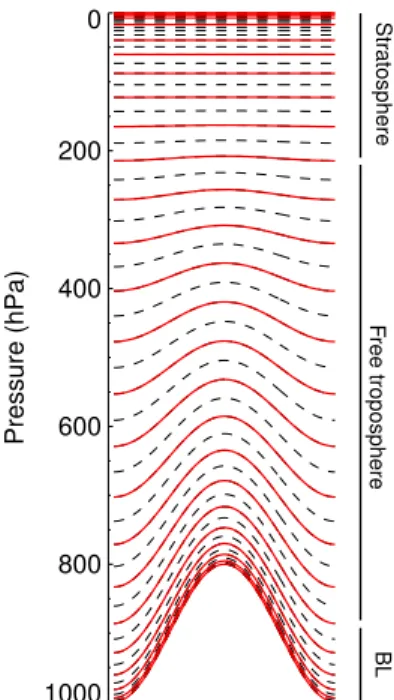
Fig. 2. Vertical resolution employed by the TM5 model. The dashed
lines represent the 60 hybrid sigma-pressure (terrain following) lev-els of the operational ECMWF model. The red solid lines repre-sent the subset employed by the 25 layer European zoom model depicted in Fig. 1. As indicated, about 5 layers represent the bound-ary layer, 10 the free troposphere, and the remaining 10 layers the stratosphere.
coarsest region represents the global domain and provides the boundary conditions for one or more nested regions. Within a nested region one or more, still finer resolved regions can be nested. Given the desired model set-up, a tree is built where for each region the parent and the children are de-fined. A region can act both as a parent and as a child. A parent provides the boundary conditions for its children and the children are used to update the information of the par-ent, which makes the nesting algorithm two-way. Figure 1 presents an example of a grid definition that has been defined to study the European area. Globally, a horizontal resolu-tion of 6◦×4◦(longitude×latitude) is employed. The Euro-pean domain is resolved at a resolution of 1◦×1◦. In order to allow a smooth transition between these two regions, a Eu-ropean domain with a resolution of 3◦×2◦has been added. This latter domain is the child of the global domain and the parent of the 1◦×1◦model area. For mass conservation it is important that the regions share a common boundary. From an algorithmic point of view, the intermediate 3◦×2◦model domain is not necessary. In practical applications, however, we always employ it to (i) study the resolution dependency of various parameterisations (ii) generate initial conditions for the underlying 1◦×1◦region (iii) avoid crude transitions from the 6◦×4◦to the 1◦×1◦domains.
Although it was shown that zooming in the vertical direction is possible when only advection processes are
<....P1 P2 P3 P4....>
C0 C1 C2 C3 C4 C5 C6 C7 C8 C9..>
Interface
Fig. 3. Schematic representation of the interface between a parent (...P1....P4...) and a child (C0....C9...). Cells C1, C2 and C3 represent the
interface cells and align with parent cell P2. The refinement factor in the depicted case equals 3.
considered (Berkvens et al., 1999), this possibility is not in-cluded because the coupling with the convection would cause severe technical problems. Therefore, all regions share the same vertical layer structure. The layers in the TM5 model are compatible with the hybrid sigma-pressure coordinate system that is employed by the ECMWF model. Thus, either the ECMWF layers are used, or some layers are combined to a coarser resolution. The current operational ECMWF model version employs 60 layers, which have been transformed into 25 model layers for the European model set-up (see Fig. 2). Since the focus of this model version is mainly on the tropo-sphere, higher vertical resolution is maintained in the bound-ary layer and in the free troposphere. Another implementa-tion of the TM5 model focuses on the stratosphere (Broek et al., 2003) and retains more vertical layers above 200 hPa.
The nesting algorithm is designed for use in combination with operator splitting. The general steps that are considered in the model are advection in the X, Y, and Z directions, pa-rameterisation of sub-grid scale mixing by deep convection and vertical diffusion (V), and chemistry (C). The latter pro-cess may include the emission and wet and dry deposition of chemical species. The operator splitting as applied in the three-region European-focused TM5 version is given in Ta-ble 1. The refinement in time relative to the global domain is 2 and 4 for regions 2 and 3, respectively. All model time steps are determined from a general time step 1T (normally 5400 s). In the global 6◦×4◦domain all numerical time steps are 1T/2. This time step is 1T/4 and 1T/8 at resolutions of 3◦×2◦and 1◦×1◦, respectively. Most meteorological infor-mation is supplied on time intervals of 6 h, while meteoro-logical information pertaining to boundary layer mixing and surface processes are provided every 3 h (see Appendix for a table that lists the TM5 input fields). These time intervals impose an upper limit to the model time step 1T. The upper part of Table 1 represents the steps that are taken in the time interval [t, t+1T/2]. The second part of the table corresponds to the interval [t+1T/2, t+1T].
If only region 1 would be considered, the model would be similar to the previous TM3 model. Numerical stud-ies have shown that the symmetrical operator splitting as applied here produces more accurate results (Strang, 1968; Berkvens et al., 2002). However, this symmetrical
split-ting can not always be preserved in the zooming algorithm. For instance, the (symmetrical) stepping order in region 1 reads XYZVCCVZYX while the order in region 2 (XYZVC-CVZYXCVZYXXYZVC) is only partly symmetrical. Such a loss of symmetry is unavoidable and the loss in accuracy is therefore hard to quantify. When communication between the parent and children occurs, this is indicated by the ar-rows in Table 1. Parents write the boundary conditions to their children (↓) whereas the parents are updated with the information calculated by their children (↑). An update of a parent involves a procedure in which the tracer masses of the parent are overwritten by information from the child cells. Likewise, boundary conditions (↓) are provided by overwrit-ing some child cells with tracer masses from the parent. Note that the algorithm allows for overlapping zoom regions, but that the results of the “last reporting” child will determine the status of the parent in the overlap zone of the children.
The mass-conserving advection algorithm that is used in the communication between parent and children has been discussed in detail by Berkvens et al. (1999). In one dimen-sion, the interface region is depicted in Fig. 3. The corre-sponding algorithm is summarized in Table 2. Cell C0 is used to store the boundary condition that is provided by the parent. The interface cells (C1, C2, and C3 in Fig. 3) are crucial in the algorithm. The sum of the masses in the in-terface cells corresponds to the mass of a parent cell and the individual cells are of child resolution. The situation appears relatively straightforward in one dimension, but complica-tions arise when the y-dimension is also considered (denoted by the “...” in Table 2). First, the boundary conditions that are written to the child may already have been advected by the parent. For instance, the tracer masses that are written to the child just before Y advection in the ↓X↓Y sequence are already advected by the parent in the X direction. Therefore, the Y interface cells of the child should not be advected again in the X direction. This is accomplished by restricting the X advection operator of the child to the core zoom region (from C4 on in Fig. 3). Second, the interface cells should operate as “parent”-like cells in one direction (e.g. X), while they should act as “child”-like cells in another advection direction (e.g. Y). In the algorithm, this is solved by “compression” of the grid in the direction of the advection (cells C1, C2, and
Table 1. Stepping order in a three-region simulation. ↓ denotes writing of boundary conditions to the children, X and Y denote horizontal
advection, Z vertical advection, V vertical diffusion and convection, and C chemistry (including emissions and deposition). ↑ represents the update parent procedure. The first and last three lines represent the first and second half of the time step, respectively.
t ... t + 1T/2 region 1 ↓X↓YZ ... VC region 2 ...↓X↓YZ...VC CVZ↓Y↓X...↑... region 3 ...XYZVC CVZYX↑...CVZYX XYZVC↑... t + 1T/2 ... t + 1T region 1 CVZ↓Y↓X... region 2 ...CVZ↓Y↓X...↓X↓YZ...VC↑ region 3 ...CVZYX XYZVC↑...XYZVC CVZYX↑...
Table 2. Schematic description of advection at the interface between parent (P) and child (C). Symbols are explained in table 1 and Fig. 3.
Step Description
1 The parent writes boundary conditions in the appropriate cells of the child (↓) P1 is copied to C0; P2 is spread over C1, C2, and C3
2 The parent is advected 1T/2 (X) 3 ....
4 The entire parent flux at the P1-P2 boundary is applied at the C0–C1 boundary of the interface cells From the C3–C4 boundary on, advection with the child time step 1T/4
5 ....
6 From the C3–C4 boundary on, a second advection step with the child time step 1T/4 Now, the flux is set to zero at the C0–C1 boundary in order to preserve mass 7 ....
8 The child cells are used to update the tracer masses of the parent (↑) P2 becomes C1+C2+C3, P3 becomes C4+C5+C6, etc.
C3 are treated as one grid cell). After advection in that direc-tion, the corresponding “decompression” is applied. More-over, after each advection step the interface cells are mixed in order to avoid negative tracer masses (C1, C2, C3 receive equal masses).
Interface cells are partially advected during some stages of the algorithm (e.g. during phase 5 of the algorithmic se-quence in Table 2). It was noted (Krol et al., 2002) that it should be avoided to perform processes like chemistry (C) and vertical mixing (V) on these partially advected interface cells. For that reason these operations on the interface cells are performed by the parent. Thus, the operations V and C are restricted to the core of the zoom region (from C4 on). In the algorithm, the parent is forced to skip only the core cells of the child region in processing the V and C steps. Af-ter a child finishes an operator sequence, the parent cells are overwritten by the child cells in an update parent procedure (↑).
2.3 Tracer transport routines
The zooming algorithm has been coupled to the slopes ad-vection scheme (Russel and Lerner, 1981). Apart from this algorithm, the second moments scheme (Prather, 1986) has been implemented for numerical studies of stratospheric transport. Due to the regular latitude longitude grid in TM5, the x-spacing of the grid becomes very small close to the poles. In order to avoid violations of the Courant-Friedrichs-Lewy (CFL) criterion in these regions, two algorithmic pro-visions have been included. First, it is possible to choose a reduced grid around the poles in the x-direction (Petersen et al., 1998). During advection in the x-direction, several grid cells are combined in the longitudinal direction and the ad-vection is performed on this coarser grid. After adad-vection, the masses of the coarse grid-cells are redistributed and the other processes are performed on the fine grid. The second provision consists of a general iteration in all advection rou-tines. Whenever a CFL criterion is violated, the time step is reduced and the same advection routine is called two (and possibly more) times.
Non resolved transport by deep and shallow cumulus con-vection has been parameterised according to Tiedtke (1989). The vertical diffusion parameterisation of Holtslag and Mo-eng (1991) is used for near surface mixing. In the free tropo-sphere, the formulation of Louis (1979) is used. To remain consistent to the meteorological input fields that are used in the model, it is important to note that these parameterisations are similar to those that are employed by the ECMWF model. One of the advantages of TM5 is that the same model is used at different resolutions. Therefore, it is considered cru-cial that the required meteorological data are consistent for the various model resolutions. Thus, the changes in the sur-face pressure should match the vertically integrated conver-gence of the mass fluxes, also within the zoom regions. As described in Sect. 2.4, meteorological pre-processing soft-ware has been developed to supply fully consistent meteo-rology at the different model resolutions.
In an intercomparison exercise of222Rn simulations with different models it was shown that the TM3 model did not capture the full diurnal cycle of near surface mixing (Den-tener et al., 1999). It was analysed that 6-h input of ECMWF was not always sufficient to describe the development of the convective boundary layer over continents. This layer re-mained systematically too shallow and it was concluded that the surface fields of latent and sensible heat fluxes should be resolved at a higher temporal resolution. As a result, too much222Rn accumulation in the surface layer over the con-tinents was observed. In order to solve this problem, the new pre-processing scheme retrieves 3-h ECMWF surface fields on a 1◦×1◦horizontal resolution. The calculation of the
dif-fusion coefficients in the boundary layer (Holtslag and Mo-eng, 1991) requires integration of these surface fields over the resolution of the region (e.g. on 6◦×4◦). These integrated fields are subsequently combined with the 6-h 3-D fields of wind shear, temperature and humidity. These latter fields re-main on a 6-h resolution to reduce data storage requirements. Surface fields also include emissions, and parameters that are relevant for deposition of trace components. Similar to the heat fluxes, these fields are stored at a resolution of 1◦×1◦ and, for the varying meteorological fields, on a 3-h basis (see table in Appendix). Prior to use in TM5, these fields are coarsened depending on the specific model set-up.
2.4 Meteorological pre-processing
The meteorological input for TM5 is created out of ECMWF data during a pre-processing stage. A complete list of TM5 input fields that are generated from ECMWF archived data is given in the Appendix. During the pre-processing stage, me-teorological fields are converted from ECMWF resolution to the TM5 grid. Horizontally, the input data is retrieved from the ECMWF archive at spectral resolution T159 or reduced Gaussian grid N80, which is equivalent to a resolution of about 1.125◦. Vertically, the data is retrieved at the 60 hybrid
sigma-pressure levels employed by the ECMWF operational model.
Although interpolation from one resolution to the other is in general straightforward, some topics will be discussed here in more detail: (i) the creation of mass fluxes, (ii) pro-duction of data for different zooming grids.
With TM5 being an Eulerian grid box model, the input re-quired for advection should consist of mass fluxes through the boundaries of each grid box cell. The procedure is de-scribed in detail in Segers et al. (2002); here a brief outline is given.
The produced mass fluxes are valid for time intervals of 6 h. The vertical mass distributions (kg air) at the begin and end of an interval are computed from the surface pressures and the hybrid coefficients of the vertical layer structure. By this, the mass change per model grid cell (kg/s) during the time interval is defined. The mass fluxes (kg/s) through the boundaries should describe how air mass is flowing from grid box to grid box, explaining the mass changes that are dictated by the changes in surface pressure. First, the vertical fluxes through the bottom of the grid boxes are computed by in-tegration of horizontal divergence, and taking into account the horizontal pressure gradients on the hybrid grid (Segers et al., 2002). Second, a first guess of the horizontal fluxes is computed from horizontal winds, which in turn are computed from the ECMWF divergence and vorticity. Finally, these first guess values are slightly modified in a way that the mod-ified horizontal fluxes and the vertical fluxes together explain the observed mass gradient. Several tests have revealed that this new pre-processing algorithm significantly improves the vertical transport in the tropopause region (Bregman et al., 2001, 2003).
To be able to run TM5 on various resolutions and for var-ious zoom definitions, the meteorological input on different resolutions should be in agreement with one another. For example, the total air mass in a 3×2 block of 1◦×1◦ cells should be equal to the the mass in the 3◦×2◦cell by which it is covered.
To achieve this, an archive has been created with meteoro-logical data on 3◦×2◦×60 resolution for 3-D fields such as
mass fluxes, temperature, and humidity. This set is used as reference for meteorological fields on other horizontal or ver-tical resolutions. For a TM5 simulation with 3-level zooming such as depicted in Fig. 1, the input is created in the follow-ing way:
– For the global 6◦×4◦ grid, the fields from the 3◦×2◦
archive are horizontally averaged, either area weighted or mass weighted. Mass fluxes through the boundaries of the boxes are simply summed.
– 3◦×2◦fields are just a subset from the archived fields.
– For 1◦×1◦fields, the meteorological fields are extracted from the raw ECMWF data, in a similar way as has been
done for the 3◦×2◦archive. However, the errors
asso-ciated with sampling the ECMWF fields depend on the resolution. In order to obtain 1◦×1◦fields that are
con-sistent with the 3◦×2◦archived fields, the 1◦×1◦fields are slightly modified, such that totals (mass fluxes) or averages (other fields) over blocks of 3×2 cells are equal to the values in the 3◦×2◦ archive. The modifi-cations that are needed are generally very small. The final step in production of the meteorological data is a reduction of the number of levels, if the model is defined on a subset of the full 60 vertical levels. Layers are combined by averaging or summing the meteorological parameters. When appropriate, weighting by the grid box masses is employed.
Creation of the 3◦×2◦×60 archive is the most expensive step in the procedure, since this requires global evaluation and interpolation of the ECMWF data. However, once this set is available, the production of data for any set of zooming area’s and/or vertical levels is rather fast, since no interpola-tion is required (6◦×4◦and 3◦×2◦grids). Processing of the 1◦×1◦regions is only required for relatively small domains.
2.5 Implementation
The entire TM5 program has been coded in Fortran 90, which allows a flexible data structure. The model has been imple-mented and tested on various platforms (IBM p690+, SGI Origin 3800, MAC OSX), including some massive parallel machines. The operational version allows the use of multi processors employing the message parsing interface (MPI).
3 Case studies
3.1 222Rn measurements on Crete
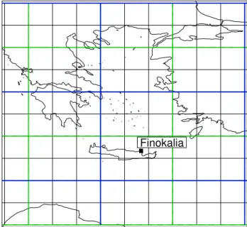
As mentioned in the introduction, the TM5 model setup is ideally suited for measurement campaigns. As an ex-ploratory example, we will analyze the 222Rn measure-ments that were made at the Finokalia station (Latitude 35◦190N, Longitude: 25◦400E) during the MINOS campaign (Lelieveld et al., 2002a). Figure 4 shows the position of the Finokalia measurement station, which is located on the island Crete in the Mediterranean sea. The station is positioned di-rectly at the coast at an altitude of 130 m above sea level. During August 2001, the dominant wind direction is from north-westerly directions and local emissions from Crete can generally be ignored (Mihalopoulos et al., 1997; Kouvarakis et al., 2000).
Figure 4 depicts the model grid of TM5 at horizontal res-olutions of 1◦×1◦, 3◦×2◦, and 6◦×4◦. On the coarsest res-olution, the Finokalia station resides in the same grid-box as the southern part of Turkey. This implies that in the model simulation with only the coarsest resolution active (i.e. no zoom regions), the222Rn emissions from Turkey (emissions are assumed to be 1.18 and 0.005 molecules cm−2s−1over
Finokalia
Fig. 4. Location of the Finokalia measurement station on Crete
along with the model at various resolutions. Blue, green, and black show the 6◦×4◦, 3◦×2◦, and 1◦×1◦horizontal resolution, respec-tively.
land and sea, respectively (Dentener et al., 1999)) are sam-pled directly by the station in the model. On 3◦×2◦the sit-uation improves, but still considerable artificial spread of the
222Rn emissions will occur. The 1◦×1◦horizontal resolution
starts to resolve the actual distribution of the land masses, although it is clear that an even higher resolution would be desirable.
We sample the station concentration in our model by three methods. A large spread among the station concentrations calculated with these three methods signals large gradients and hence a large sampling error. The first sampling method simply takes the average mixing ratio of a tracer in the grid box. The second method employs the simulated values of the x, y, and z-slopes (Russel and Lerner, 1981) together with the mean mixing ratio to interpolate to the station location, when this location is not in the center of the grid. The third method uses bilinear interpolation with the adjacent grid-cells in the x, y, and z directions. In this method, the value of the tracer slopes within a grid cell are not used. For the simulation on 6◦×4◦, large sampling errors are encountered (often >20%, not shown). The situation improves if the zoom regions are activated. In the 1◦×1◦ simulation, difference in the sam-pling methods only arise if large concentration gradients are present close to the station (e.g. around 21 August, as dis-cussed below).
In Fig. 5 the222Rn concentrations simulated during Au-gust 2001 are compared to the measurements. A spin-up time of one month was used and bilinear interpolation was employed to calculate the concentration at the location of Fi-nokalia. The simulated station concentrations with only the
01-Aug 06-Aug 11-Aug 16-Aug 21-Aug 26-Aug 01-Sep 2001 0 50 100 150 200 222 Rn (pCu/SCM) 3x2 6x4 1x1
Fig. 5. TM5 model simulations of222Rn compared to 2-h mea-surements (red crosses). Blue, green and black refer to a horizontal resolution of 6◦×4◦, 3◦×2◦, and 1◦×1◦, respectively. The grey bar indicates the time period with low wind speed.
01-Aug 06-Aug 11-Aug 16-Aug 21-Aug 26-Aug 01-Sep
2001 20 40 60 80 100 120 222 Rn (pCu/SCM)
Fig. 6. TM5 model simulations of222Rn compared to measure-ments (red crosses). The black line is the same as in Fig. 5 and the blue line refers to an artificial station 1◦ north of Finokalia. The grey bar indicates the time period with low wind speed.
global 6◦×4◦ resolution active, are systematically too high due to the emissions from the land masses that reside in the same grid box as the sampling station. The situation im-proves when the 3◦×2◦European zoom domain is used and an even better agreement is obtained when also the 1◦×1◦ zoom region is used. Obviously, the match between measure-ments and model is still not perfect, but this example shows that the model results can improve considerably with higher model resolution.
The largest deviations between the 1◦×1◦simulation and the measurements are observed around 21 August (see grey bar in Figs. 5–7), when the model overestimates the222Rn concentration by more than 50 pCu/SCM. In Fig. 6 the sim-ulated concentrations are shown (in blue) for a location 1◦ north of Finokalia. While for most of the simulation period the differences are small, it can be observed that the
simu-5 10
Windspeed (m/s)
01-Aug 06-Aug 11-Aug 16-Aug 21-Aug 26-Aug 31-Aug
2001 0 200 400 600 800
Boundary layer height (m)
250 300 350
Winddirection (degrees)
Fig. 7. Meteorological analysis at the Finokalia station during the
MINOS campaign. The brown lines in the upper and middle panel denote the measured wind speed and direction, respectively. The thick black lines are the 6-h wind speed and direction interpolated at the Finokalia station. The blue lines are interpolated to an arti-ficial station one degree north of Finokalia. In the lower panel the modeled boundary layer heights are plotted for the two locations. The grey bar indicates the time period with low wind speed.
lated concentrations around 21 August at open sea are dras-tically lower. To analyse the situation in more detail, Fig. 7 shows the measured wind speed and direction along with the ECMWF values that are employed by the TM5 model. These values have been interpolated from the mass fluxes at the borders of the grid boxes. In order to exclude the influence of the island of Crete on these interpolated values, the wind data have also been analysed at a position one degree north of Finokalia. At this northerly position the measured wind speed is well reproduced by the mass fluxes derived from the ECMWF data. Not surprisingly given the location of the station, the measured wind speed at Finokalia appears to be representative for open sea. The measured wind direction is
systematically more westerly than the wind direction in the model. This is most likely caused by local effects. At the coast, the airflow is forced upward or sideward, which re-sulted in a backing of the wind direction. From the wind measurements and simulations, the situation around 21 Au-gust stands out as a period of low wind speeds (gray bar). During such a period, the influence of Cretean emissions on the simulated222Rn concentration increases. The222Rn accumulation is reinforced by the shallow boundary layer heights that are calculated during this period (see Fig. 7). Since over sea most of the solar heat flux generates evapo-ration, the depth of the boundary layer is predominantly de-termined by the vertical wind shear. Inspection of the lower panel in Fig. 7 reveals that around 21 August, the boundary layer height collapses to about 100 m due to the low wind speeds. The grid box in which Finokalia resides contains about 30% land masses, and a diurnal cycle in the calculated boundary layer height can be observed. Nevertheless, the boundary layer calculated by the TM5 model (and also by the ECMWF model) are very shallow. Inspection of the potential temperature profiles that were measured during the MINOS aircraft flights reveals a stable profile with several stronger inversions. One inversion layer is normally located between a few hundred and 1000 m. Other inversions are found higher up, normally between 1 and 3 km, but the situation appears quite variable. In general it can be stated that vertical mixing is not very strong due to a stable temperature profile that is associated with subsiding air motions.
From the analysis presented here, it appears that measure-ments of wind data and other meteorological parameters, in-cluding boundary layer heights, are (potentially) very impor-tant in the validation of the model results. Unfortunately, these meteorological parameters are not always measured during field campaigns and at long term measurement sta-tions.
Additional validation of the TM5 transport using 222Rn measurements has been performed in a recent methane inver-sion paper (Bergamaschi et al., 2005). Within the EU frame-work 5 project EVERGREEN (EnVisat for Environmental Regulation of GREENhouse gases) a detailed comparison between various transport models is performed, including the transport of 222Rn with prescribed emissions. TM5 is performing well, especially within the European zoom do-main. The correlation between daily averaged measurements and TM5 output ranges between 0.5 (Zugspitze) and 0.8 (Freiburg).
As an example, we show in Fig. 8 the comparison be-tween TM5 and measurements at Mace Head in two peri-ods in 2001. Linear interpolation to the station location has been used. In both periods we observe sampling problems when the model is sampled at the position of the Mace Head measurement station (red lines). This is attributed to the di-rect222Rn emissions in the sampling gridbox and the adja-cent gridboxes that are used for the lineair interpolation. If the sampling location is moved two grid-boxes westwards
Jan/Feb
0 10 20 30 40 50 0 1 2 3 4 5 Rn [Bq /m ] 222 3 Rn [Bq /m ] 222 3Jul/Aug
190 200 210 220 230 240 0 1 2 3 4 5 Day in 2001Fig. 8. TM5 model simulations of222Rn compared to measure-ments taken at Mace Head (Ireland, see Fig. 1) during two bi-monthly periods in 2001. The red line represents hourly averaged model output interpolated at the Mace Head location. The blue line represents model output interpolated to a position two degrees to the west to avoid the direct influence of222Rn emissions from land masses. The black dots are the hourly measurements and the bars represent daily averages with 1σ standard deviation.
(blue lines), the comparison between model and measure-ments significantly improves. These conclusions are in line with Chevillard et al. (2002) and Peters et al. (2004) who discussed similar sampling problems and stressed the impli-cations for inverse modelling studies.
3.2 Effects of zooming on the transport of chemical trace species
As noted in the previous section, pronounced improvements can be achieved by resolving the interaction between emis-sions and transport of222Rn at a higher horizontal resolution. The artificial spread of local emissions is reduced and grid-boxes become more representative of the actual situation at sampling stations. Thus, the advantages of the local higher resolution are clear. Now, the question arises what the effects are of using a coarse grid outside the zoom region. Related to
10
010
110
210
310
410
5L1 (ppt)
0
2
4
6
8
10
Production L20L1 (kg/kg)
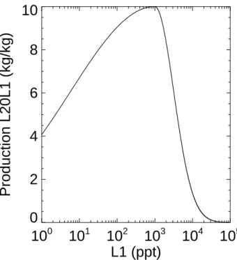
Fig. 9. Artificial non-linear chemical production curve of L20L1
as a function of the L1 concentration. The maximum value of 10, for instance, implies that for each molecule of L1 that is lost at a concentration of 1000 ppt, a chemical production of 10 L20L1 molecules has been applied.
this: why would a one-way nested zooming algorithm not be sufficient? To explore these questions we introduced some artificial tracers in TM5. These tracers mimic some features of tropospheric ozone chemistry, however, without the de-tailed chemical feedback mechanisms. Tracer L1 (“NOx”)
and L20 (“CO”) are emitted using an emission distribution and strength comparable of that of NOx as given by the
EDGAR3.2 inventory (Olivier and Berdowski, 2001). To mimic the chemical breakdown of NOx and CO, a simple
radioactive decay (with lifetimes of 1 and 20 days, respec-tively) has been applied to the tracers L1 and L20. Further-more, an artificial tracer L20L1 (“O3”) is introduced that is,
like O3, not emitted, but only chemically produced. The
pro-duction of L20L1 is coupled to the decay of tracer L1 and this production depends non-linearly on the L1 concentra-tion. Figure 9 depicts the assumed L20L1 production effi-ciency as a function of the L1 concentration. The curve con-sists of two linked Gaussian curves which are given by:
L1 > 1000 ppt : 10 exp −(log(L1)−3)0.5 2 (1)
L1 ≤ 1000 ppt : 10 exp −(log(L1)−3)10.0 2. (2) At L1 concentrations of about 1000 ppt, the L20L1 produc-tion is assumed to be the most efficient (10 molecules L20L1 per lost L1 molecule). At lower and higher L1 concen-trations, the L20L1 production levels off, an effect that is
stronger towards higher L1 concentrations. In this way, the resolution effects on the L1 concentrations are non-linearly translated into L20L1 production rates and concentrations. The lifetime of L20L1 has been taken as 20 days. As men-tioned above, the L20L1 production curve can be interpreted as representative for NOxdependent ozone production in the
atmosphere. More rigorous attempts to study the resolution dependence of atmospheric chemistry are outside the scope of this paper. The L20L1 tracer is merely used to study mech-anisms that lead to differences in simulations with non-linear chemistry. Specifically, the effects of zooming and two-way (versus one-way) nesting are investigated.
In order to study the effects of two-way versus one-way nesting, several simulations are compared. The simulations are all initialized by fields that are taken from a yearly 6◦×4◦ only simulation. In a first simulation (R3), the European zoom domain of Fig. 1 is employed in a two month sim-ulation (July and August 2001). In a second simulation (R5), a second zoom domain over North America (3◦×2◦, and 1◦×1◦) is also activated. Due to less artificial mix-ing of the L1 emissions in the North American zoom re-gion (on a 6◦×4◦resolution the emissions are directly spread over a large area), the L1 concentration distribution becomes broader. Specifically, more grid cells will fall in the high con-centration end of the curve depicted in Fig. 9. As a result, the non-linear production of L20L1 differs and these differences are still present outside the North American zoom region be-cause two-way nesting is employed. This is illustrated in Fig. 10, which shows the comparison in the lowest model layer after two months of simulation. The figure is the last frame of a movie that animates daily plots of the L20L1 sur-face concentrations. The movie is discussed in more detail in the Appendix. The upper panel represents the simula-tion with only the European zoom domains active (R3). In the middle panel the zoom over North America is also ac-tivated (R5) and the lower panel depicts the differences (in %) between the two simulations. The difference plot within the North American zoom region signals large differences in the L20L1 concentrations that are the direct consequence of less artificial spread of L1 emissions in the R5 simula-tion. In the case of one-way nesting, these differences would have been confined to the zoom domain. Because of the two-way nesting, however, the differences also occur outside the North American zoom region, for instance in Europe. Within the European zoom domain the differences disappear quite rapidly for two reasons. First, the lifetime of the L20L1 is limited to 20 days and the budget over Europe is dominated by local L20L1 production. Second, horizontal and verti-cal transport processes dilute the L20L1 concentration fields which causes annihilation of the negative and positive de-viations. The consequence is that, when the concentrations are sampled at Mace Head (see Fig. 11), the differences be-tween the R5 and R3 simulations are relatively small (usually smaller than 10%). Interestingly, the R5 simulation produces systematically lower L20L1 concentrations at Mace Head.
Fig. 10. The last frame of a movie (see Appendix) that depicts the simulated L20L1 concentration in the lowest model layer. The upper panel
shows the simulation with only the European zoom domains active (R3, the location of the zoom regions is denoted by the white frames). The middle panel shows the simulation with also the North American zoom domain active (R5). The lower panel depicts the % difference calculated as 100(R5–R3)/R5. Here, the focus is on the area outside the American zoom region.
As mentioned before, more grid cells fall in the high concen-tration end of the curve depicted in Fig. 9 when the North American resolved at 1◦×1◦. Consequently, less L20L1 is produced and transported towards Europe.
The differences between the R5 simulation and the sim-ulation with only the European zoom at 3◦×2◦ active (R2,
green), and the simulation with no zoom regions at all (R1, blue) are also shown in Fig. 11. These differences are usu-ally much larger. This means that, at least for this artificial chemistry case, the “gain” of a better local representation (i.e. a reduction of the sampling error and better resolved trans-port and emissions) is larger than the loss in accuracy that is caused by grid-coarsening at some distance from the mea-surement station. This observation is in line with the intuitive argument that it seems not logical to resolve the atmospheric
transport and chemistry globally at a high resolution when the focus is on the local situation.
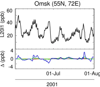
A similar conclusion can be drawn from the concentrations that are sampled at a station positioned in Omsk (see Fig. 1), east of the European zoom domain (Fig. 12). Since this lo-cation falls outside all zoom regions, the concentrations are only available only on the 6◦×4◦model grid for all
experi-ments (R1, R2, R3, R5). The differences between R5 (top panel) and R3 (lower panel, red) are very small. Thus the concentrations as simulated at Omsk are hardly influenced by the presence of the North American zoom region. The ef-fects of European zooming (R2 and R3) are only marginally larger, but may reach 10% if the European resolution is de-graded to 6◦×4◦(R1, blue line).
Mace Head (9.9W, 53.3N)
10
20
30
40
50
L20l1 (ppb)
01-Jul
01-Aug
2001
-20
0
20
∆
(ppb)
Fig. 11. Upper panel: the simulated L20L1 concentration as a
func-tion of time at stafunc-tion Mace Head (Ireland, see Fig. 1) for the sim-ulation with both the North American and European zoom domain activated (R5). The lower panel shows the concentration differences with three other simulations. Red: only the European zoom ac-tive (R3). Green: only the European zoom at 3◦×2◦active (R2). Blue: no zoom regions active (R1). A value smaller than zero in the lower panel implies that the R5 simulation produces higher concen-trations.
Table 3. Budget in August 2001 of tracer L20L1 in the
atmo-spheric boundary layer (surface–850 hPa) between 30◦N and 90◦N for the different simulations in 109moles L20L1. R1 means only global 6◦×4◦; R2: +European zoom 3◦×2◦; R3: +European zoom 1◦×1◦; R5: +two North American zoom region on 3◦×2◦ and 1◦×1◦. “Initial” and “Final” refer to the burden at the beginning and end of August, respectively. y and z refer to the net trans-port in the latitudional and vertical directions. “Conv”: convection;
Pchem:chemical production; Lchem:chemical loss.
Initial y z Conv Pchem Lchem Final
R1 94 −69 −118 −212 +560 −154 102 R2 93 −66 −129 −204 +558 −152 101 R3 92 −65 −133 −198 +555 −150 101 R5 90 −61 −142 −176 +529 −145 96
In order to check the importance of the various processes, a TM5 simulation is accompanied by a budget calculation. For the simulations described here, the budget of the bound-ary layer in the northern mid and high latitudes (between 30◦N and 90◦N) is analyzed. The values of the individual budget terms will depend on whether or not zoom regions are present. Table 3 lists the individual budget terms for the vari-ous model simulations. Note that the initial conditions in the table already differ, because the simulation spans two months
Omsk (55N, 72E)
20
40
60
L20l1 (ppb)
01-Jul
01-Aug
2001
-4
0
4
∆
(ppb)
Fig. 12. Upper panel: the simulated L20L1 concentration as a
func-tion of time at stafunc-tion Omsk (Russia, see Fig. 1) locafunc-tion for the simulation with both the North American and European zoom do-main activated (R5). The lower panel shows the concentration dif-ferences with three other simulations. Red: only the European zoom active (R3). Green: only the European zoom at 3◦×2◦active (R2). Blue: no zoom regions active (R1). A value lower than zero in the lower panel implies that the R5 simulation produces higher concen-trations.
Table 4. Budget in August 2001 of tracer L20 in 109 moles. “Emis”: emission. Other symbols: see header Table 3.
Initial y z Conv Emis Lchem Final
R1 17 −11 −23 −92 +154 −28 18 R2 17 −10 −26 −90 +154 −27 18 R3 17 −10 −28 −88 +154 −27 18 R5 16 −8 −33 −85 +154 −26 17
and the budget is shown for the second month. As outlined above, it is observed that zooming changes the production (and thus the concentration) of chemically active tracers in a systematic way. Interestingly, relative large changes in the vertical transport are observed. With coarser resolution, the convection parameterization appears to be more effective in venting the boundary layer. With higher resolution, however, the less effective convection is partly compensated by en-hanced advective vertical transport. This is expected, since the vertical motions that are associated with frontal systems are better resolved.
The same resolution dependencies are seen in the budgets of tracers L20 (see Table 4) and L1 (not shown). In more re-alistic atmospheric chemistry simulations these effects will also be present, although they may be obscured by feed-back processes. For instance, the simulated concentration of
the hydroxyl radical concentration (OH) will depend on the model resolution. As a consequence, the lifetime of methane and other gases will also change with the grid size.
In general, the effects of model resolution on transport and specifically sub-grid vertical mixing has been poorly ex-plored in global atmospheric chemistry studies. This exam-ple demonstrates the power of the TM5 model to quantify resolution dependent effects in a consistent and systematic way.
4 Conclusions
TM5 extends the functionality of TM3 by the possibility to zoom over specific regions. In this way, a local high resolu-tion is achieved while the computaresolu-tional costs remain rela-tively low. The major advantage of a local high resolution is that the model grid cells are more representative for the lo-cations at which measurements are taken, as was shown by the222Rn study presented in Sect. 3.1. Boundary conditions, which are important for longer lived species, are provided in a natural way, i.e. by a simulation on the parent grid which is run simultaneously. In the present study, regions with a high-est horizontal resolution of 1◦×1◦are employed, but the al-gorithm can easily be used for higher horizontal resolutions. The TM5 model is ideally suited for budget studies. The import and export budgets of specific regions can be stud-ied as was highlighted by the artificial tracer study sented in Sect. 3.2. With such studies in mind, we have pre-defined zoom regions over Europe, North America, Africa and Asia (see http://www.phys.uu.nl/∼tm5). In this way,
global “hot-spots” of atmospheric chemistry (high emission rates of ozone precursors) can be resolved at higher resolu-tion without dramatically increasing the computaresolu-tional costs. Other ongoing efforts with the TM5 model include the cou-pling with forecast meteorology in order to provide chemical forecasts (chemical weather) and the use of TM5 in inverse modelling studies. The use of two-way nesting is impor-tant for inverse modeling studies since emissions, resolved at higher resolution within zoom regions, influence the sim-ulated concentrations also outside these regions. Synthesis inversions that optimize emissions of trace gases by min-imizing the differences between simulations and measure-ments will therefore benefit from the two-way nesting ap-proach (Bergamaschi et al., 2004). To further assist inverse modelling studies, the adjoint version of the TM5 transport routines have been coded and been used to calculate the sen-sitivity of specific measurements for upwind emissions (Gros et al., 2003, 2004). Additionally, the global transport of TM5 has been validated using SF6 measurements (Peters et al.,
2004). Finally, TM5 can be used to study the resolution de-pendence of processes. In Sect. 3.2 these effects were quan-tified by activating and deactivating zoom regions. Specifi-cally the vertical mixing processes were shown to depend on resolution.
Appendix
Movie (http://www.copernicus.org/EGU/acp/acpd/4/3975/ acpd-4-3975-mv01.mov) of daily L20L1 concentrations in the lowest model layer. The upper panel (R3) only the European zoom is active. In the middle panel (R5) the North American zoom regions are activated. The lowest panel depicts the differences (%) defined as 100(R5–R3)/R5.
Description of the movie
In the upper panel of the frames (R3) the North Amer-ican zoom domain is not present. As a result, the L20L1 concentration fields retain the 6×4 block structure over this region throughout the movie. After a few days, the patterns of L20L1 over North America in the R5 simulation show more fine structure, with higher maxima (e.g. 15 June, 28 June, 19 July at the East Coast, 23 July in Central USA). Interestingly, at the west coast of the USA, the R5 simulation clearly shows systematically lower L20L1 concentrations. In that region, L1 is emitted in relatively stagnant air (Los Angeles area). The L1 concentrations in the high resolution R5 simulation reach very high levels, i.e. beyond the concentrations at which L20L1 is produced most efficiently (1000 ppt, see Fig. 9). In the R3 simulation, artificial spread of the L1 emissions leads to spurious dilution and hence lower L1 concentrations over the emission hot-spots. As a result, systematically less L20L1 is produced in the R5 simulation. Clearly, the interaction between meteorology and emissions plays an important role in the non-linear chemical production of L20L1 (and ozone). At the east coast, both the meteorological variability and the area with substantial L1 emissions are larger.
The main transport routes out of the North American zoom region are to the north-east towards Europe and to the south-west towards the Pacific. These transport events are variable and depend strongly on the atmospheric circulation. Trans-port events are clearly visible in the difference plot that is depicted in the lower panel. Due to less production of L20L1 in the R5 simulation, it appears as if the negative deviations are transported out of the North American domain. Differ-ences as large as −10% are seen towards Europe (25 June, 7 July, 11 July, 30 July) and the Central Pacific (20 June, 1 July, 30 July).
Because of two-way nesting, air flowing out from a zoom domain may flow in again later. This is most clearly ob-served in the difference movie, where the perturbations seem to “flow in” at the south-eastern side of the North American domain. From the difference movie it is also clear that the differences between the R3 and R5 simulations are generally small over most of Asia and Russia.
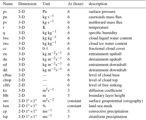
Table 5. Overview of the TM5 input fields that are produced using ECMWF data. 2-D refers to latitude×longitude fields. 3-D fields are
resolved in height. Fields associated with boundary layer diffusion and the surface fields are resolved with a 3-h resolution. Fields related to surface processes are resolved at a spatial resolution of 1◦×1◦.
Name Dimension Unit 1t (hour) description ps 2-D Pa 6 surface pressure pu 3-D kg s−1 6 eastwards mass flux pv 3-D kg s−1 6 northward mass flux t 3-D K 6 temperature q 3-D kg kg−1 6 specific humidity lwc 3-D kg kg−1 6 cloud liquid water content iwc 3-D kg kg−1 6 cloud ice water content cc 3-D 0-1 6 fractional cloud cover eu 3-D kg m−2s−1 6 entrainment updraft du 3-D kg m−2s−1 6 detrainment updraft ed 3-D kg m−2s−1 6 entrainment downdraft dd 3-D kg m−2s−1 6 detrainment downdraft clbas 2-D — 6 level of cloud base cltop 2-D — 6 level of cloud top cllfs 2-D — 6 level of free sinking kz 3-D m2s−1 3 diffusion coefficient blh 2-D m 3 boundary layer height
oro 2-D 1◦×1◦ m2s−2 constant surface geopotential (orography) lsm 2-D 1◦×1◦ % constant land-sea mask
cp 2-D 1◦×1◦ ms−1 3 convective precipitation lsp 2-D 1◦×1◦ ms−1 3 stratiform precipitation
TM5 input fields
Table 5 lists the TM5 input fields. These fields are produced in a pre-processing step (see Sect. 2.4) that uses ECMWF data. Only a subset of all the surface fields is listed. The complete set of surface fields contains parameters that are needed for deposition calculations, such as surface roughness, surface stress, sea ice, etc.
Acknowledgements. Financial support for M. Krol was provided
by the European FP5 project PHOENICS. M. Botchev, P. Berkvens and J. Verwer are acknowledged for their work on the numerical foundations of the zoom algorithm. Computer facilities were provided by the Dutch NCF (Nationale computerfaciliteiten). S. Wagner is acknowledged for his constructive comments on the manuscript. N. Mihalopoulos (ECPL, University at Crete) is acknowledged for providing the 222Rn measurements from Finokalia. The long term monitoring program ORE-RAMCES and LSCE are acknowledged for providing the Mace Head222Rn measurements.
Edited by: M. Heimann
References
Bauer, S. E. and Langmann, B.: Analysis of a summer smog episode in the Berlin-Brandenburg region with a nested atmosphere-chemistry model, Atmos. Chem. Phys., 2, 259–270, 2002,
SRef-ID: 1680-7324/acp/2002-2-259.
Bergamaschi, P., Hein, R., Heimann, M., and Crutzen, P. J.: Inverse modeling of the global CO cycle 1. Inversion of CO mixing ra-tios, J. Geophys. Res., 105, 1909–1927, 2000.
Bergamaschi, P., Behrend, H., and Jol, A.: Inverse modelling of national and EU greenhouse gas emission inventories, report of the workshop “Inverse modelling for potential verification of na-tional and EU bottom-up GHG inventories”, Tech. Rep., Joint Research Centre, Ispra, Italy, ISBN 92-894-7455-6, 2004. Bergamaschi, P., Krol, M., Dentener, F., Vermeulen, A., Meinhardt,
F., Graul, R., Ramonet. M., Peters, W., and Dlugokencky, E. J.: Inverse modelling of national and European CH4emissions
us-ing the atmospheric zoom model TM5, Atmos. Chem. Phys. Dis-cuss., in press, 2005.
Berkvens, P. J. F., Botchev, M. A., Lioen, W. M., and Verwer, J. G.: A zooming technique for wind transport of air pollution, MAS-R9921, 31, CWI, Amsterdam, 1999.
Berkvens, P. J. F., Botchev, M. A., Krol, M. C., Peters, W., and Verwer, J. G.: Solving vertical transport and chemistry in air pol-lution models, in Atmospheric Modelling, edited by D. Chock and G. Carmichal, 130 of IMA Volumes in Mathematics and its Applications, 1–20, Springer, Berlin, 2002.
Bousquet, P., Peylin, P., Ciais, P., Quere, C. L., Friedlingstein, P., and Tans, P. P.: Regional changes in carbon dioxide fluxes of land and oceans since 1980, Science, 290, 1342–1346, 2000. Bregman, A., Krol, M. C., Teyss`edre, H., Norton, W. A., Iwi, A.,
Chipperfield, M., Pitari, G., Sundet, J. K., and Lelieveld, J.: Chemistry-transport model comparison with ozone observations in the midlatitude lowermost stratosphere, J. Geophys. Res., 106, 17 479–17 496, 2001.
Bregman, B., Segers, A., Krol, M., Meijer, E., and Velthoven, P. v.: On the use of mass-conserving wind fields in chemistry-transport models, Atmos. Chem. Phys., 3, 447–457, 2003,
SRef-ID: 1680-7324/acp/2003-3-447.
Broek, M. M. P. v. d., Aalst, M. K. v., Bregman, A., Krol, M., Lelieveld, J., Toon, G. C., Garcelon, S., Hansford, G. M., Jones, R. L., and Gardiner, T. D.: The impact of model grid zooming on tracer transport in the 1999/2000 Arctic polar vortex, Atmos. Chem. Phys., 3, 1833–1847, 2003,
SRef-ID: 1680-7324/acp/2003-3-1833.
Chevillard, A., Ciais, P., Karstens, U., Heimann, M., Schmidt, M., Levin, I., Jacob, D., and Podzun, R.: Transport of222Rn using the regional model REMO: A detailed comparison with measure-ments over Europe, Tellus, 54B, 872–894, 2002.
Cosme, E., Genthon, C., Martinerie, P., Boucher, O., and Pham, M.: The sulfer cycle at high-southern latitudes in the LMD-ZT General Circulation Model, J. Geophys. Res., 107, 4690, doi:10.1029/2002JD002 149, 2002.
Cotton, W. R., Pielke, R. A., Walko, R. L., Liston, G. E., Tremback, C. J., Jiang, H., McAnelly, R. L., Harrington, J. Y., Nicholls, M. E., Carrio, G. G., and McFadden, J. P.: RAMS 2001: Current status and future directions, Meteorol. Atmos. Phys., 82, 5–29, 2003.
Dentener, F., Weele, M. v., Krol, M., Houweling, S., and Velthoven, P. v.: Trends and inter-annual variability of methane emis-sions derived from 1979–1993 global CTM simulations, Atmos. Chem. Phys., 3, 73–88, 2003,
SRef-ID: 1680-7324/acp/2003-3-73.
Dentener, F. J., Feichter, J., and Jeuken, A. B. M.: Simulation of transport of222Rn using on-line and off-line global models at different horizontal resolutions, Tellus, 51B, 572–602, 1999. Dlugokencky, E., Houweling, S., Bruhwiler, L., Masarie, K. A.,
Lang, P. M., Miller, J. B., and Tans, P. P.: Atmospheric methane levels off: Temporary pause or a new steady-state?, Geophys. Res. Lett., 20, 1992, doi:10.1029/2003GL018 126, 2003. Frohn, L. M., Christensen, J. H., Geels, J., Brandt, C., and Hansen,
K. M.: Validation of a 3-D hemispheric nested air pollution model, Atmos. Chem. Phys. Discuss., 3, 3543–3588, 2003,
SRef-ID: 1680-7375/acpd/2003-3-3543.
Grell, G. A., Emeis, S., Stockwell, W. R., Schoenemeyer, T., Forkel, R., Michalakes, J., Knoche, R., and Seidl, W.: Application of a multiscale, coupled MM5/chemistry model to the complex terrain of the VOTALP valley campaign, Atmos. Environ., 34, 1435–1453, 2000.
Gros, V., Williams, J., Aardenne, J. A. v., Salisbury, G., Hofmann, R., Lawrence, M. G., Kuhlmann, R. v., Lelieveld, J., Krol, M., Berresheim, H., Lobert, J. M., and Atlas, E.: Origin of anthro-pogenic hydrocarbons and halocarbons measured in the summer-time European outflow (on Crete in 2001), Atmos. Chem. Phys., 3, 1223–1235, 2003,
SRef-ID: 1680-7324/acp/2003-3-1223.
Gros, V., Williams, J., Lawrence, M., Kuhlmann, R. v., Aar-denne, J. v., Atlas, E., Chuck, A., Edwards, D. P., Stroud, V., and Krol, M.: Tracing the Origin and Ages of Interlaced At-mospheric Pollution Events over the Tropical Atlantic Ocean with in situ Measurements, Satellites, Trajectories, Emission In-ventories and Global Models, J. Geophys. Res., 109, 22 306, doi:10.1029/2004JD004846, 2004.
Heimann, M., Monfray, P., and Polian, G.: Long-range transport of
222Rn – a test for 3D tracer models, Chem. Geol., 70, 98–98,
1988.
Holtslag, A. A. M. and Moeng, C.-H.: Eddy diffusivity and counter-gradient transport in the convective atmospheric boundary layer, J. Atmos. Sci., 48, 1690–1698, 1991.
Houweling, S., Dentener, F., and Lelieveld, J.: The impact of non-methane hydrocarbon compounds on tropospheric photochem-istry, J. Geophys. Res., 103, 10 637–10 696, 1998.
Houweling, S., Kaminski, T., Dentener, F., Lelieveld, J., and Heimann, M.: Inverse modeling of methane sources and sinks using the adjoint of a global transport model, J. Geophys. Res., 104, 26 137–26 160, 1999.
Jacob, D. J., Crawford, J. H., Kleb, M. M., Connors, V. S., Bendura, R. J., Raper, J. L., Sachse, G. W., Gille, J. C., Emmons, L., and Heald, C. L.: Transport and chemical evolution over the Pacific (TRACE-P) aircraft mission: Design, execution, and first results, J. Geophys. Res., 108, 8781, doi:10.1029/2002JD003 276, 2003. Jonson, J. E., Sundet, J. K., and Tarras´on, L.: Model calculations of present and future levels of ozone and ozone precursors with a global and a regional model, Atmos. Environ., 35, 525–537, 2001.
Kaminski, T., Heimann, M., and Giering, T.: A coarse grid three-dimensional global inverse model of the atmospheric transport, 2, Inversion of the transport of CO2in the 1980s, J. Geophys.
Res., 104, 18 555–18 581, 1999.
Kouvarakis, G., Tsigaridis, K., Kanakidou, M., and Mihalopoulos, N.: Temporal variations of surface regional background ozone over Crete Island in the southeast Mediterranean, J. Geophys. Res., 105, 4399–4407, 2000.
Krol, M., Peters, W., Berkvens, P., and Botchev, M.: A new al-gorithm for two-way nesting in global models: principles and applications, in: Proceedings 2nd Int. Conf. Air Pollution Mod-elling and Simulation, April 9–12, 2001, edited by: Sportisse, B., 225–235, Springer, Berlin, Heidelberg and New York, 2002. Krol, M. C., Lelieveld, J., Sturrock, G., Penkett, S., Brenninkmeijer,
C., Gros, V., Williams, J., and Scheeren, H.: Continuing emis-sions of methyl chloroform from Europe, Nature, 421, 131–135, 2003.
Langmann, B., Bauer, S. E., and Bey, I.: The influence of the global photochemical composition of the troposphere on Euro-pean smog, Part I, Application of a global to mesoscale model chain, J. Geophys. Res., 108, 4146, doi:10.1029/2002JD002 072, 2003.
Lelieveld, J., Berresheim, H., Borrmann, P. J. C. S., Dentener, F. J., Fischer, H., Feichter, J., Flatau, P. J., Heland, J., Korrmann, R. H. R., Lawrence, M. G., Levin, Z., Markowicz, K. M., Mi-halopoulos, N., Minikin, A., Ramanathan, V., M, d., Roelofs, G. J., Scheeren, H. A., Sciare, J., Schlager, H., Schultz, M., Siegmund, P., Steil, B., Stephanou, E. G., Stier, P., M, M. T., Warneke, C., Williams, J., and Ziereis, H.: Global air pollu-tion crossroads over the Mediterranean, Science, 298, 794–799,