Approximate cross validation for sparse generalized linear models

Approximate Cross Validation for Sparse

Generalized Linear Models

by

William T. Stephenson

Submitted to the Department of Electrical Engineering and Computer

Science

in partial fulfillment of the requirements for the degree of

Master of Science

at the

MASSACHUSETTS INSTITUTE OF TECHNOLOGY

February 2019

@

Massachusetts Institute of Technology 2019. All rights reserved.

<Signature redacted,

A uthor ..

...

Department of Electrical Engineering and Computer Science

Signature redacted

January

4, 2019

C ertified by ...

...

Tamara Broderick

Assistant Professor of Electrical Engineering and Computer Science

Thesis Supervisor

Signature redacted

Accepted by ...

'

Lesl(e"A Kolodziejski

QO' JECHNLOWGY

_{Professor of Electrical Engineering and Computer Science}

FE 2

17

219I

Chair, Department Committee on Graduate Students

LIBRARIES

Approximate Cross Validation for Sparse Generalized Linear

Models

by

William T. Stephenson

Submitted to the Department of Electrical Engineering and Computer Science on January 4, 2019, in partial fulfillment of the

requirements for the degree of Master of Science

Abstract

Cross validation (CV) is an effective yet computationally expensive tool for assessing the out of sample error for many methods in machine learning and statistics. Previous work has shown that methods to approximate CV can be very accurate and computa-tionally cheap, but only for low dimensional problems. In this thesis, a modification of existing methods is developed to extend the high accuracy of these techniques to high dimensional settings.

Thesis Supervisor: Tamara Broderick

Contents

1 Introduction

9

2 Overview of Approximation 13

2.1 Approximate CV with f1 Regularization ... 15

3 Bounds on Approximation Quality 19 3.1 Primal dual witnesses and support recovery . . . . 19

3.2 Conditions under which ||ng||I" < 1 . . . ... 20

3.3 Linear Regression . . . . 23

3.4 Logistic Regression . . . . 24

3.5 Conditions under which supp 0 = supp 0* . . . . 25

4 Experiments 27 4.1 Two alternatives to Eq. (2.5) . . . . 27

4.2 The importance of correct support recovery . . . . 28

4.3 Real data experiments . . . . 31

4.4 Selection of A and future work . . . . 32

A Differences between Eq. (2.2) and Eq. (2.3) 35 A.1 Derivation of "simple" approximation . . . . 35

A.2 Derivation of "modified" approximation . . . . 36

A.3 Comparison of approximations . . . . 36

C Proofs from Chapter 3

C.1 Local structured smoothness condition (LSSC) C.2 Linear Regression . . . .

C.3 Linear regression: minimum eigenvalue . . . .

C.4 Linear regression: incoherence . . . .

C.5 Linear regression: bounded gradient . . . .

C.6 Linear regression: A small enough . . . .

C.7 Logistic Regression . . . . C.8 Logistic regression: lambda min . . . . C.9 Logistic regression: incoherence . . . .

C.10 Logistic regression: bounded gradient . . . . .

C.11 Logistic regression: A small enough . . . .

41 . . . . 42

. .. .

43

45 .. . . 47

51

. . . .

53

. . . .

53

. . . . 54

. . . .

55

55

. . . .

56

List of Figures

1-1 Scaling of existing methods for approximate cross validation for un-regularized linear regression. When the dimension D of the regres-sion parameters is in constant ratio with the number of observations,

D/N = 1/10, we see that the approximation error goes down at the

(1/v/'N-) rate described in [12]. With a fixed dimension of D = 2,

however, we see the error goes down at the significantly faster rate of

O(1/N 2) as described in [2]. We describe conditions under which we

can recover the same O(1/N2) for a dimension that grows as o(eN). . 10

4-1 (Left:) Accuracy of experiments from Section 4.1. Percent error is

computed as in Eq. (4.1). Note the error in Eq. (2.5) (red curve) is not noticeable but is nonzero: it varies between -0.06% and 0.04%.

(Right:) Timings of results from Section 4.1. The legend is the same

as on the left, with the addition of blue showing the runtime of exact

CV for the f, regularized model (the D x D matrix inversion needed

for approximating CV in the smoothed problem is so slow that even exact CV with an efficient f, solver is faster). . . . . 28

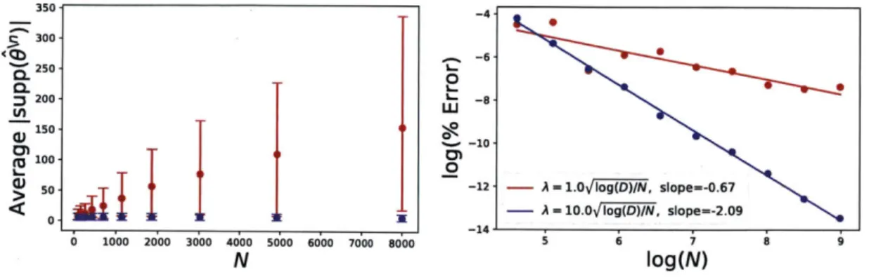
4-2 Illustration of the role of support recovery in the accuracy of the ap-proximation in Eq. (2.5) in the case of linear regression. On the left, we show the average Isupp \nI1, with the average taken over a few ran-dom values of n and error bars showing the min and max

I

supp \n

I .

For A = 10.0 log(D)/N, the mean recovered support remains con-stant with N. On the other hand, for A = 1.0 /log(D)/N, Jsupp O\nI is growing with N, as well as hugely varying for different values of n. As a result, we are forced to approximate the behavior of a much higher dimensional optimization problem. The right plot shows the resulting reduced accuracy in terms of Eq. (4.1) as D scales with N: when the support recovery is constant, we recover an error scaling of 0(1/N2

),

whereas a growing support results in a much slower decay. . . . . 29

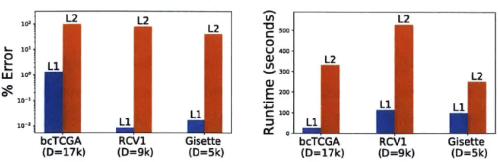
4-3 (Left:) Accuracy for real data experiments in Section 4.3. For each

dataset, we give the accuracy of approximate CV compared to exact

CV for both f2 regularized models using the existing Eq. (2.2) and

f, regularized models using our proposed Eq. (2.5). We compute "%

Error" as in Eq. (4.1). (Right:) Timings for the same experiments. . 31

4-4 Experiment for selecting A from Section 4.4. (Left:) Despite being

very accurate for higher values of A, approximate CV's degredation in accuracy for lower values of A (which corresponds to a larger S) causes the selection of a A that is far from optimal in terms of test loss.

(Right:) For a lower dimensional problem, the curve constructed by

approximate CV much more closely mirrors that of exact CV for all values of A. . . . . 33

Chapter 1

Introduction

Cross validation is a useful tool for assessing the accuracy of many methods in machine learning and statistics. Although generically applicable and straightforward to use, it has the downside of requiring many re-fittings of the same model. As machine learning models often use as much computation as possible, even a single fitting can be very time consuming. To this end, practitioners typically use k-fold CV with a small k (e.g., five or ten), as this only requires k re-fittings of the model. While k-fold

CV is more computationally efficient, leave-1-out CV is known to be asymptotically

more accurate for assessing the out of sample error [3, 1]. Unfortunately, leave-1-out

CV is hugely computationally expensive, as it requires N refittings, where N is the

number of observed datapoints.

To this end, the topic of approximate leave-1-out CV has recently become an active area of research [2, 12, 17, 4]. The core methods proposed by these four works are fairly similar (see Chapter 2 for an overview), have been shown to be empirically successful, and some work has been done to show their accuracy theoretically. [2] demonstrate that, given both the parameter-space and data-space are bounded, the approximation error is Op(1/N2), for the amount of data N growing and the dimension

of the parameter 0 to be estimated, D = dim9, staying fixed.

[12]

make some less and some more restrictive assumptions than

[2]

and are able to recover an error scaling of Op(1/V) for the high-dimensional case of D/N converging to a constant. Finally, with the exception of assuming a fixed dimension,

[4]

make the least restrictive

LJ -l CD -0 -12-- D Fixed, slope--2.02 -14- D Growing, slope=-0.56 4.5 5.0 5.5 6.0 6.5 7.0 7.5 8.0 8.5 log(N)

Figure 1-1: Scaling of existing methods for approximate cross validation for

unreg-ularized linear regression. When the dimension D of the regression parameters is in constant ratio with the number of observations, D/N = 1/10, we see that the

ap-proximation error goes down at the 0(1/V/W) rate described in [12]. With a fixed dimension of D - 2, however, we see the error goes down at the significantly faster rate of 0(1/N2_{) as described in [2]. We describe conditions under which we can}

recover the same 0(1/N2_{) for a dimension that grows as}

o(eN).

assumptions, and obtain an error rate of O(1/N).

Our key takeaway from the above works is that all recently studied approaches to approximate cross-validation are very accurate with a small, fixed dimension, but have either unstudied or significantly reduced accuracy when the dimension of the parameters is high relative to the amount of data; see Fig. 1-1 for an illustration of this in the case of linear regression. We argue that this is a fairly important point, as the major cases of interest when N is large are also high dimensional. In particular, if

N is significantly larger than D, the training loss is usually a good approximation to

the test error, and any form of CV is relatively unnecessary; for example, well known results in empirical risk minimization imply that, for fixed dimension, the training error fairly quickly approaches the true error (see, e.g., [14]).

A common theme in high dimensional statistics and machine learning is to assume

that a high dimensional problem really has a much lower "effective dimension." For example, the high dimensional data may be low rank, or the true parameter underlying the data may be sparse. Since parameter estimation can be made significantly more accurate in the presence of such low effective dimension, one might wonder if the same can be said of approximate CV. The example in Fig. 1-1 provides evidence that this

is not immediately true: the higher dimensional problem shown there (the blue line) has a sparse true parameter but still suffers from a reduction in accuracy.

Our main contribution is to demonstrate one case in which this notion of effective dimension is helpful for approximate CV - that of f, regularized generalized linear models (GLMs) with data generated by a sparse parameter. The theoretical proper-ties of f, regularization and other sparsity inducing regularizers has been extensively studied [11, 10, 8, 16]; it is generally shown that, under certain conditions on the amount of regularization and the structure of the problem, the recovered parameter 0 is very accurate and/or has the correct support. Drawing on this body of work, we show that f, regularized GLMs have special structure that is not present when using other regularizers that allows approximate CV methods to be highly accurate, even when the dimension grows with N. In particular, we propose a modification of existing approximations and prove conditions under which it successfully takes ad-vantage of the sparse structure in f, regularized problems to obtain an accuracy and computational expense equivalent to that of a small, fixed dimensional problem. As a major step along the way, we prove conditions under which the exact solution to the

f1 regularized problem remains stable as each datapoint is held out. In experiments with synthetic and real data, we show that this increased accuracy and decreased runtime is realized in practice: the sparsity of f, regularized problems allows our approximation to be significantly more accurate and quicker compared to existing approximate CV methods run with different regularizers on the same data.

Chapter 2

Overview of Approximation

At the heart of all previous approximate cross validation methods is a linear approx-imation to the solution 9 of the optimization problem:

9 A arg min F(9) + AR(9), (2.1)

OERD

where A > 0 is a regularization parameter, R : RD -R R is some regularization

function, and F : RD -+ *R is some function that decomposes into N terms: F(O) =

(1/N) EN_1

fn(9).

In this work, we focus on the case of generalized linear models

(GLMs), in which

F(O) = (1/N)

En

f(xn',

yn), where Xn E RD and yn E R are

observed data. Let 9\n be the solution to the same problem with the nth datapoint held out and H(6) the Hessian of F + AR evaluated at 6. Then, if we assume f and R are twice differentiable and F(O) + AR(9) is strongly convex at 9, the following

approach from

[4]

gives an approximation 6\n to 6\":

:= - H()- nf(49, yn). (2.2)

An alternative is to use the approach given by [2, 12, 17]:

In general, this approach requires the inversion of a D x D matrix per each 6\n evaluated, whereas Eq. (2.2) only requires a single inversion to evaluate all 6\n. In general, this is a O(ND) computational cost to evaluate all 6\n by Eq. (2.3) versus a O(D3

+

ND2_{) cost for using Eq. (2.2) (one matrix inversion plus N matrix}

mul-tiplications). In the special case of generalized linear models, each V2f is actually a rank one matrix, so standard rank-one update formulas give that only one inver-sion is required; see Appendix A for a derivation and discusinver-sion of both approaches. Looking forward to more general cases, however, we prefer to study the generally computationally cheaper approach given by Eq. (2.2). We stress, though, that even a single inversion of a D x D matrix can be very expensive, as the time complexity of O(D3) and memory usage of O(D2_{) quickly become prohibitively expensive for D} in the tens of thousands.

Even if both approximations were computationally cheap in high dimensions, there is a further issue: their accuracy is much poorer in high dimensions. As noted above, Fig. 1-1 shows that, for a fixed dimensional parameter D = dim9 = 2, the approxi-mation error in Eq. (2.2) goes down as O(1/N2

), whereas for a growing dimension,

D/N

= 1/10, the error only decays as O(1/v1/). For D much larger than N, we

expect the error to stay constant or even grow.

The above observations about computational expense and statistical accuracy can ruin the original point of these types of approximations. Specifically, the original hope is that, for a small fixed computational budget, using Eq. (2.2) or Eq. (2.3) will be significantly more accurate than, say, running k-fold CV or sub-sampling leave-1-out. The above discussion tells us that in high dimensions, a) computing Eq. (2.2) or Eq. (2.3) is probably impossible on a small budget, and b) has dubious usefulness anyway. This motivates our main observation in the next section: through appropriate use of f regularization, we can retain the

0(1/N

2_{) scaling and low computational}

2.1

Approximate CV with f, Regularization

A common assumption in high dimensional settings is that only a small number of

dimensions of each x, are actually relevant for predicting the outcomes y,; that is, there exists some 9* such that |supp9*| j SI is much smaller than D. One of the most popular choices for R in such settings is R(9) = 110|1, (a.k.a., "the Lasso") due

to its excellent empirical and theoretical properties. Intuitively, it typically correctly recovers supp 9 = supp9*, at which point Eq. (2.1) is reduced to a ISI, rather than

D, dimensional problem.

Unfortunately, Eq. (2.2) is not immediately applicable when R = .-

i,

as this choice of R is not twice-differentiable. One suggestion put forward by [17, 12] is to use Eq. (2.3) with a smoothed approximation of

110111.

A less obvious alternative,

also given by [17, 12], is to observe that Eq. (2.3) has a closed form as the amount of smoothness goes to zero. While technically one can use a large amount of smoothing to achieve the same effect, we find that this is not achievable in practice due to numerical issues; see Section 4.1 for an empirical illustration. Below, we make two observations about this limiting argument: 1) the same argument immediately applies to the generally more computationally efficient Eq. (2.2), and 2) the limiting version has better statistical and computational properties than a smoothed version of Eq. (2.2).

In order to state this more formally, let S supp 6 be the support recovered by the full f, regularized optimization problem, X E RNxD the data matrix with rows

Xn, X.,g its submatrix formed by taking only the columns in

5,

and finally define

(2) A d2_{f (z,yn)}

_(2.4)

Theorem 1.

Define the restricted Hessian of F as H gg A XT

diag

(2) )X. g, and assume without loss of generality that S = {1, 2, ... ,|\}. If Hg has strictly positive eigenvalues and one considers any "reasonable" smooth approximation to

11111

and

takes the limit as the amount of smoothness goes to zero, the limit of Eq. (2.2) is:

(O"

0,

-

H-

[Vof(x.

, y)

₍₂₅

s s . (2.5)

SC0

Furthermore, this limiting approximation has the following properties:

1. It has the same computational expense as an SI-dimensional version of Eq. (2.2).

2. If the conditions discussed Proposition 2 hold for the full data problem, and those discussed in Proposition 1 hold for each of the leave-1-out problems, then the error in Eq. (2.5) behaves as if the underlying problem were

I

SI dimensional.

Proof. That Eq. (2.5) is the limit of a smoothed version of Eq. (2.2) follows directly

from the arguments in either of [17, 12], who derive the limit of a smoothed approx-imation to Eq. (2.3) (and also give precise meaning to a "reasonable" smoothing of

110111). The point about computation follows by noting Eq. (2.5) only acts along

SI1

dimensions, which tells us that we only need to invert and perform multiplications with a

SI1

x

SI1,

rather than D x D, matrix. The point about accuracy follows from Proposition 1 and Proposition 2, which together imply that 1) all leave-i-out problems are really optimization problems restricted to the dimensions S (i.e., supp $\n

c

and 2) the approximation in Eq. (2.5) runs over only these dimensions. E The most important step in proving this theorem is giving conditions under which

Eq. (2.1) and each of the leave-1-out problems are actually

I

SI-dimensional

optimiza-tion problems and our approximaoptimiza-tion acts only along these dimensions. After having shown this, the conclusions 1) and 2) in its statement are immediate: the accuracy and computational expense behave as if we were dealing with a |I-dimensional, rather than D-dimensional, problem because we actually are dealing with a I -dimensional problem.

Of course, Theorem 1 is not particularly useful if its conditions are not satisfied by practical examples. The most difficult to check are the conditions of

(X, Y), these conditions are satisfied for linear and logistic regression with very high

Chapter 3

Bounds on Approximation Quality

One of the properties that has made the use of f, regularization so popular is that, given a true parameter 0* E RD with supp 0* = S such that ISI

<

D, the optimal solution 0 to Eq. (2.1) often has supp 0 = S, even when N

<

D. In this section we will show an important piece of the proof of Theorem 1: conditions under which not only supp 0 = S, but also supp = supp 0 -\ = S. We start by reviewing a common

technique for proving the support recovery properties of f1 regularized problems. Notably, these proofs proceed by showing that solving f1 regularized problems is actually the same as solving a ISI-dimensional problem, which exactly fits with the discussion right after Theorem 1 above.

3.1

Primal dual witnesses and support recovery

At the heart of many proofs for showing that f, regularized problems recover the correct support S = supp 0* is a proof showing that the solution to a lower dimensional optimization problem is the unique solution to Eq. (2.5) [16, 8, 10]. The idea is to consider the "oracle estimator," which for S' being the complement of S, sets &sc = 0,

and 0s as the solution to the restricted version of Eq. (2.1)1:

N

0s = argmin

f(xsOsyn)

+A

I0sI

₁

.

(3.1)

OsERISI n=1

If this problem is strongly convex, this 0s is unique. If 9 = (Os, 0) satisfies the

first order optimality conditions for the un-restricted problem:

Vof (Xiyn) +A2 = 0, (3.2)

n

where 2 is some element of the subdifferential 8|111, then this 0 is also an optimal solution to Eq. (2.1). The main difficulty comes in showing that this 0 is the unique optimal solution. One condition for this is given by a lemma from [61:

Lemma 1 (Lemma 11.2 from [6]). If the 2 satisfying the first order optimality

con-ditions Eq. (3.2) also satisfies ||Esc|| < 1, then the oracle-estimated 0 is the unique

optimal solution to Eq. (2.1). That is, we have supp 0 C supp 9*. This has an immediate corollary relevant to our problem:

Corollary 1. Let \n satisfy the first order optimality conditions Eq. (3.2) for the

nth leave-1-out problem. If maxn||2|||x < 1, then all the leave-1-out problems are

really optimization problems in the same |SI dimensional space.

Even for just the original problem, it is not obvious that 1I sc

K,

< 1 will hold in many situations; a large amount of work has gone into identifying conditions for which this holds high probability for various M-estimators. After reviewing a recent version of these conditions, we describe our main insight: that the conditions under which it holds for all leave-1-out problems are almost identical to those for the full data problem.

3.2

Conditions under which

||s\"||oo

<

1

Conditions under which | zsc

II,

< 1 holds vary throughout the literature. Studying

specialized to f1 regularized linear regression. [8] generalizes this argument to other M-estimators, as well as other types of regularization. Most recently, [101 gave conditions specific to f, regularization, but that allow for a wide class of M-estimators. We find the conditions in [10] to be the easiest to check as each datapoint is held out and so choose to work with them here. The main result from [10] is:

Proposition 1 (Theorem 5.1 from [101). For defined in Eq. (3.2),

II|sctK'

< 1 if

the following conditions hold:

1. (LSSC) F satisfies the (0*, No.) locally structured smoothness condition with constant K. This condition, proposed by [10], is not required to understand our results, so we defer its definition to Appendix C.1.

2. (Strong convexity) The restricted problem Eq. (3.1) is strongly convex:

Amin (V2 F(9*)ss) Amin > 0 (3.3)

for some

Amin-3. (Incoherence) A less interpretable, but common in the literature, condition is the incoherence condition:

VF(*)sc,s (72F(*)ss) 1 < 1 - (3.4)

for some y > 0.

4.

(Bounded gradient) The gradient of F evaluated at the true parameters 6* is small relative to the amount of regularization:

IIVF(6*)IK

<

₄

A

(3.5)

5. (A is sufficiently small) The above are satisfiable with a regularization parameter that is not too large:

A

2

i

A m (3.6)

with the understanding that puts no constraint on A if K = 0.

An immediate consequence is that, if each of these conditions hold for each Fn(0),

then we have |Czf| < 1 for each datapoint n. The proofs of Theorem 2 and Theorem 3 take the obvious approach of checking that the conditions in Proposition 1 are true for each of the leave-1-out problems. This will require conditions on the data matrix X; intuitively, one might imagine that if one of its rows x, were particularly "extreme," the conditions of Proposition 1 will not be satisfied for F\n. While all our results could be given explicitly in terms of the entries of X, they are not especially interpretable in this form. Instead, we will assume a particular random form for X and study what happens as D and N grow. In particular, we will assume throughout that the data matrix X is comprised of i.i.d. sub-Gaussian entries:

Definition 1. [Sub-Gaussian random variable

[15]

A random variable X is

sub-Gaussian with parameter c, > 0 if:

E exp

x2

< 2.

(3.7)

Our results will be stated both in terms of the sub-Gaussian parameters of the data as well as various global constants all of which will be denoted by C > 0; these constants are related to various relationships between sub-Gaussian random variables and are completely independent of the problem. We note that high probability results for random data are in some sense the best sort of result one might hope to get about the stability of f1 regularization under leave-1-out. Specifically, the results of [18] imply that there exist worst-case training datasets (X, Y) for which sparsity inducing methods like f, regularization are not stable as each datapoint is left out. In this sense, our Theorem 2 and Theorem 3 can be interpreted as showing that f, regularizaion is stable with high probability. In any case, in order to make such an analysis we will

need one major assumption:

probability for the full data problem:

Pr

[

VF(*)sc,s

(V2F(*)ss) < 1 - 7/ < e2 5

for some fixed y > 0, where the probability is taken over the random data X, Y.

In general, there is not much understanding of when Eq. (3.4) holds, let alone when it holds with high probability as in Assumption 1. It seems to be standard to assume that Eq. (3.4) holds (starting from its introduction in [19] and continuing in more recent work [8, 10]); we make the somewhat stronger assumption that the condition holds with high probability under a random sub-Gaussian design matrix. While we will not attempt to prove Assumption 1, it is worth noting that it is known to hold for the simplified case of linear regression with an i.i.d. Gaussian design matrix

(e.g., see exercise 11.5 of [6]).

3.3

Linear Regression

Under such a random design, we can show that Li regularized linear regression recovers the same support as each datapoint is left out with high probability; we do so by checking that the conditions stated in Proposition 1 hold for each leave-1-out problem. Specifically, assume a linear regression model y,, =

x7'O*

+ wn, where x, E RD has i.i.d. cr-sub-Gaussian components with E[xd] = 1 and wa is cm-sub-Gaussian. We then have the following:

Theorem 2. Assume that Assumption 1 holds and that D, as a function of N,

grows as o(eN). Consider the linear regression model above, and set the regularization parameter as:

1 clc, log D 25csc, 4cc.(log(ND) +26)

A

= __

+

+

(3.8)

where C > 0 is a global constant, and Ml is defined as:

|S|I2cM log(s(D- NS

ISI

+ V2Ccx logN)

M _{= 0}

(for a non-big-O statement, see Appendix C). Then each of the leave-1-out problems has supp 6\n C _{S with a high, fixed probability. That is,}

Pr [max S =i1

<

22e2 5 (3.9)

Proof. We check that, for the value of A given in the theorem statement, the conditions

of Proposition 1 are all satisfied with probability at least 1 - 22e-2 . See Theorem 4 in Appendix C for details.

It is worth noting how the A given in Eq. (3.8) compares to that typically given for successful support recovery for the original 0. Theorem 11.3 of [6J gives the commonly stated condition A > O( log(D)/N) as sufficient for ensuring that supp b C S with

high probability in the case of linear regression. Although this is true for any scaling of D and

N,

the error in 0, 110 - 6*112, is usually proportional to A, so to have asymptotically decaying error in b, one needs D = o(eN). This same scaling is relevant in Theorem 2: if D = o(eN) and we additionally assume that ISI is a constant, we get Mj = o(1), so that the A we require is also O( log(D)/N). In this sense, if some A is large enough to guarantee support recovery and good squared error error in the original problem, using A + o(1) gives support recovery for all of the leave-1-out problems.

3.4

Logistic Regression

We can next state a very similar result for logistic regression. Assume a logistic

regression model such that the data yn

E

{-1, 1} with Pr [y, = 1] = 1/(1 + e-x ) where xn E RD has i.i.d. cx-sub-Gaussian components.

Theorem 3. Assume that Assumption 1 holds and that D, as a function of N, grows

as o(eN). Consider the logistic regression model above, and set the regularization parameter as:

1

25 + log D

2c7

log(ND) + v/5(c.1

A = - gD+.(3.10)

a - Mi

NC

N(a - Mj)

where C is a global constant relating to relationships between sub-Gaussian random variables, and Mj is defined as in Theorem 2. Then each of the leave-1-out problems has support supp 6\n C S with a high, fixed probability. That is,

Pr

[max

S =

1]

< 28e- 5 (3.11)

L n o

Proof. The proof runs very similarly to that of Theorem 2; see Theorem 5 in

Ap-pendix C for details. E

A similar analysis of the A required by Theorem 3 applies here, as [10] show that

A > O( log(D)/N) is sufficient to ensure good squared error and accurate support recovery of 6.

3.5

Conditions under which supp

0

= supp

0*

We have just seen that, in the case of linear and logistic regression, if a particular A is sufficient for ensuring

IIssc

< 1, a slightly increased A is sufficient for ensuring

maxn

I|zSIIc

< 1. According to Lemma 1, this condition ensures that supp 6\n c

supp 9* for all n; however, this is not enough to establish Theorem 1. The issue is

that our approximation in Eq. (2.5) only runs over the dimensions in S. If S is a

strict subset of the true S, it is possible that, for some n, we will have S C supp

$\'

so that our approximation does not cover the extra dimensions in 6\'. However, a

commonly stated condition ensures S = S:

that is

min|6*1 > -\/I-I 7+4 (3.12)

'sES S Amin

where -y and Amin are as defined in Proposition 1 for the full data problem, and also

assume

IIsciK

< 1. Then supp6 = supp 0.

Proof. This is part of Theorem 5.1 in [101.

We note that this is not an extra condition beyond that required for the success of the original estimate 0; conditions on the minimum entries of 6* are typically used in the f, literature to ensure S = S (e.g., in [8, 10, 16]), and Eq. (3.12) is an exact duplicate of the condition in [10].

Assuming the conditions of Proposition 2 hold, Theorem 2 and Theorem 3 now tell us that we can expect our approximation in Eq. (2.5) to be highly accurate and computationally cheap, even when the dimension D grows as o(e N).

Chapter 4

Experiments

4.1

Two alternatives to Eq. (2.5)

Our theoretical results imply that Eq. (2.5), derived by using a smooth approximation to the f, norm with Eq. (2.2) and then taking the amount of smoothness to zero, has high accuracy and low computational cost. We begin our empirical investigation of this claim by first considering two more straightforward alternatives: 1) ignore the limiting argument and just use Eq. (2.2) with some smoothed version of 110111, or 2) approximate exact CV by exactly computing 9\" for just a few random values of

n. For the former point, we consider the smooth approximation R7(0) for 77 > 0

suggested by [12]:

RI()

: log(1 + e40d) + log(1 + e~70d)

d=1

While limc0 Rq(O) = 110111, we found this approximation to become numerically

unstable for the purposes of optimization when T was much larger than 100, so we set q = 100 in our experiments. To test this along with subsampling exact CV, we

trained logistic regression models on twenty five high dimensional random datasets in which Xnd i N(0, 1) with N = 500 and D = 40, 000, and the true 0* was supported on its first five entries. We compute the accuracy of our various approximations to

1750-20 1500-0 0 1250-- -1000-LUW

750-~-40

W " -60 - - Appx Ll - Appx Smooth Li 250

-S0 - Exact Subsamp. -_10CoAI I

0 5 10 15 20 25 0 5 10 15 20 25

Trial number Trial number

Figure 4-1: (Left:) Accuracy of experiments from Section 4.1. Percent error is com-puted as in Eq. (4.1). Note the error in Eq. (2.5) (red curve) is not noticeable but is nonzero: it varies between -0.06% and 0.04%. (Right:) Timings of results from Section 4.1. The legend is the same as on the left, with the addition of blue showing the runtime of exact CV for the i regularized model (the D x D matrix inversion needed for approximating CV in the smoothed problem is so slow that even exact CV with an efficient f, solver is faster).

full exact CV as the percent error of exact CV:

japproximation - exactCVI (4.1)

exactCV

Fig. 4-1 shows the accuracy of these two alternatives to Eq. (2.5), and Fig. 4-1 com-pares their timings. By design, subsampling exact CV has almost exactly the same runtime as using Eq. (2.5)1; however, we see that its accuracy is significantly reduced for nearly every trial. Using Eq. (2.2) with R10 0(0) as a regularizer is far worse:

while subsampling exact CV is fast and unbiased (although very high variance), the smoothed approximation has to deal with a the full D x D matrix and an approxima-tion over all D dimensions, resulting in an approximaapproxima-tion that is orders of magnitude less accurate and slower.

4.2

The importance of correct support recovery

The discussion in Chapter 3 revolved around the point that each

$\n

having correct support (i.e. supp 0\n = supp 0*) was sufficient for obtaining the fixed-dimensional

'Specifically, we computed 41 different $\n for each trial in order to roughly match the compu-tational cost of computing Eq. (2.5) for all N = 500 datapoints.

350 300 250 200 150 100 50

d

3 -4. -6-L. 0 L-a--12 - A - 1.0lVog(D)/N, slope=-0.67 - A = 10.0]Iog(D)/N, slope.-2.09 0 1000 2000 3000 4000 5000 6000 7000 8000 iog(N) N log(N)

Figure 4-2: Illustration of the role of support recovery in the accuracy of the ap-proximation in Eq. (2.5) in the case of linear regression. On the left, we show the average |supp \|, _{with the average taken over a few random values of n and error} bars showing the min and max Isupp O\"|. For A = 10.0 Vlog(D)/N, the mean

recov-ered support remains constant with N. On the other hand, for A = 1.0 1log(D)/N,

|supp

$\"

is growing with N, as well as hugely varying for different values of n. As a result, we are forced to approximate the behavior of a much higher dimensional optimization problem. The right plot shows the resulting reduced accuracy in terms of Eq. (4.1) as D scales with N: when the support recovery is constant, we recover an error scaling of O(1/N2_{), whereas a growing support results in a much slower decay.} error scaling shown in Fig. 1-1. Here, we give some brief empirical evidence that this is actually necessary, at least in the case of linear regression. For values of N ranging from 1,000 to 8,000, we set D =

FN/10

and generate a design matrix with i.i.d. N(0, 1) entries. The true 0* is supported on its first five entries, with the rest set to zero. We then generate observations y, = xn96

+

wn, for w, rlZ9

N(0, 1). To

examine what happens when the recovered supports are and are not correct, we use slightly different values of the regularization parameter A. Specifically, the results of

[16] (especially Theorem 1) tell us that the support recovery of f, regularized linear

regression will change sharply around A ~ 4 log(D)/N, where lower values of A will fail to correctly recover the support.

With this in mind, we choose two settings of A: 1.0

log(D)/N

and 10.0

log(D)/N.

As expected, the righthand side of Fig. 4-2 shows that the quality of the approxima-tion in Eq. (2.5) is drastically different in these two situaapproxima-tions. The lefthand plot of Fig. 4-2 offers an explanation for this observation: the support of supp 0\" grows with N under the former value of A, whereas the latter value of A ensures that

Isupp \"| = Jsupp 9* = const. Empirically, this confirms the idea that accurate

support recovery of each \n is also necessary to recover the "low-dimensional" error

scaling described in Fig. 1-1.

That the approximation quality relies so heavily on the exact setting of A is some-what concerning. However, we emphasize that this is just as much a criticism of

f, regularization in general; as previously noted, [16] demonstrated similarly drastic

behavior of supp 0 in the same exact linear regression setup that we use here. On the other hand,

[7]

do show that, despite this sensitive behavior, using exact leave-1-out

CV to select A for f, regularized linear regression does give reasonable results. In

Section 4.4, we empirically show that this is sometimes, but not always, the case for our and other approximate CV methods.

102 L2 L2 2 A L2 L2 a500-C 0 202 Uo 400-0 _{4 L2} L1 U L_ Li in..-L2 WJ 100-30 _L 10-1 _Li L Li 100 1o, Li

1

Li

bcTCGA RCV1 Gisette bcTCGA RCV1 Gisette

(D=17k) (D=9k) (D=5k) (D=17k) (D=9k) (D=5k)

Figure 4-3: (Left:) Accuracy for real data experiments in Section 4.3. For each dataset, we give the accuracy of approximate CV compared to exact CV for both f2

regularized models using the existing Eq. (2.2) and f, regularized models using our

proposed Eq. (2.5). We compute "% Error" as in Eq. (4.1). (Right:) Timings for the

same experiments.

4.3

Real data experiments

While we have shown increased accuracy of Eq. (2.5) on synthetic data, it is important to understand how dependent our results are on the particular random design we chose. We explore this question by running on a number of publicly available datasets. We chose the particular datasets shown here for having a high enough dimension to observe the effect of our results, yet not so high in dimension nor number of datapoints that running exact CV for comparison was prohibitively expensive. For a description of each dataset as well as our exact experimental setup, see Appendix B. For each dataset, we approximate CV for the f, regularized model using Eq. (2.5). To understand how Eq. (2.5)'s accuracy is improved by the special structure present in f, regularized problems, we compare to the accuracy of the approximation in Eq. (2.2) on the same problem, but with 2 regularization, in which there is no sparsity, and the approximation runs over all D dimensions. The accuracy we report on the left of Fig. 4-3 is the percent error compared to exact CV as in Eq. (4.1). Our results, reported in Fig. 4-3 show that approximate CV on the f, regularized problem is significantly more accurate. Additionally, the timings on the right of show in Fig.

4-3, show that the approximations to the f, regularized problems have significantly

4.4

Selection of A and future work

Most previous work in approximate CV, including ours, has focused on showing that with a fixed model with increasing amounts of data, N, (or, in the case of our approx-imation, both increasing N and D), approximate CV will give an accurate assessment of the out of sample error. However, this does not address one of the more common uses of CV, which is to train many models with varying values of the regularization parameter A and select the one with the lowest CV error. We consider this issue here. We generate a synthetic f, regularized logistic regression problem with N = 300

observations and D = 150 dimensions. The data matrix X has N(0, 1) entries, and

the true 0* is supported on only its first five entries. As a measure of the "true" out of sample error, we construct a test set with ten thousand observations. For a range of values of A, we solve Eq. (2.1), and measure the train, test, exact leave-1-out, and approximate leave-1-out errors; the results are plotted in Fig. 4-4. Not only does our approximate CV select a A that gives a significantly worse test error than exact CV, it selects the obviously incorrect value of A = 0.0. This issue is somewhat suggested by

our theory above: that is, for an appropriately large A, we will recover a small, correct support S and approximate CV will be highly accurate, whereas small A will cause a larger support S, which in turn causes a degredation in approximation quality. While the results in Fig. 4-4 come from using our Eq. (2.5) to approximate CV for an ii. regularized problem, we note that this issue is not specific to the current work; we observed similar behavior when using f2 regularization with both Eq. (2.2) and the

computationally slower Eq. (2.3).

Still, all is not lost for approximate CV: the righthand side Fig. 4-4 shows that for the same problem setup with D = 75 dimensions, the error vs A curve constructed by approximate CV is significantly different. In particular, it is convex and has its

minimum very close to that of exact CV. We believe a further understanding of this issue is the most pressing direction for future work. In the meantime, this failure mode of approximate CV is at least easy to spot, assuming one believes that the true out of sample error is a convex function of A.

N=300, D=150 Train Loss --- Test Loss --- Exact CV - Appx. CV 1.0

A

1.25 1.50 1.75 2.00 0.8. N=300, D=75 0 L. 0.7-0.6. 0.5- 0.4- 0.3-0.00 0.2s O.5O 0.75 1.0 1.2s 1.50 1.7s 2.0

'A

Figure 4-4: Experiment for selecting A from Section 4.4. (Left:) Despite being very accurate for higher values of A, approximate CV's degredation in accuracy for lower values of A (which corresponds to a larger S) causes the selection of a A that is far from optimal in terms of test loss. (Right:) For a lower dimensional problem, the curve constructed by approximate CV much more closely mirrors that of exact CV for all values of A.

L-0 L. 0.7- 0.6- 0.5- 0.4- 0.3- 0.2-0.00 0.2 O.5o 0.7s Train Loss -Test Loss -- Exact CV - Appx. CV

Appendix A

Differences between Eq. (2.2) and

Eq. (2.3)

In Chapter 2, we briefly outlined the differences between Eq. (2.2) and Eq. (2.3); we examine the differences in more detail here. Recall that we defined H($) A

(1/N)

zsN

₁Vf(x 7', yn). We restate the "simple" approximation given by

[4]

as:

(A.1)

whereas the "modified" approximation given by [2, 12, 17] is:

-

(

₎ - VYf(x0, y)) Vof(x $, yN).

(A.2)

A.1

Derivation of "simple" approximation

[4] derive Eq. (A.1) by appealing to the implicit function theorem. Specifically, they

define 6^w as the solution to a weighted optimization problem:

Aarg min - n n Y) (

OEDNn=1

(A.3)

For example, Leave-1-out CV with the first datapoint left out corresponds to solving

Eq. (A.3) with w = (0,1,1, ... , 1). [4] note that the derivatives of 9 (i.e. the solution

to Eq. (A.3) with w = 1) with respect to the weights wn, can be computed using the implicit function theorem to get:

dO

-

-H(9)-lVof(xT,

y ).

(A.4)

dwnWn=1n

By a first order Taylor expansion around w = (1,1,..., 1), we can write:

N^

O'W ~~ + E d6n W=(Wn -)(

A.5)

n=1

N

= 9 - H()-lVof (x ,

yn)(wn

-1). (A.6)

For the special case of w being the vector of all l's with a zero in one coordinate (i.e. the weighting for leave-1-out CV), we recover Eq. (A.1).

A.2

Derivation of "modified" approximation

Eq. (A.2) is derived by taking a single Newton step on the objective F\n starting at

the point 9. Specifically, recall that the objective with one datapoint left out is:

F\

(0)

=

N

f(X4,

yn)

-

Nf(x

,

y),

(A.7)

n=1

which has V2F\n(0) =

H(0)

- V2f(X4, yn) as its Hessian. This gives a single Newton step from the point 0 as exactly Eq. (A.2).

A.3

Comparison of approximations

There is a major computational difference between Eq. (A.2) and Eq. (A.1): the former requires the inversion of a D x D matrix for each \n approximated, while the latter requires a single D x D matrix inversion for all

$\n

inverted, which incurs a cost

of O(N

+

ND3) versus a cost of O(N

+

D3). Even for small D, this is a significant additional expense.

However, as noted by [12, 171, Eq. (A.2) is much cheaper when considering the special case of generalized linear models. In this case, Vjf is some scalar times Tnn -a rank one matrix. The Sherman-Morrison formula then allows us to cheaply compute the needed inverse in Eq. (A.2) given only H-1; this is how Equation 8 in

[121 and Equation 21 in [17] are derived. Even though we only consider GLMs in this work, we, as noted above, still prefer to study Eq. (A.1) with the hope of retaining scalibility in more general problems.

Appendix B

Details of real experiments

We use three publicly available datasets for our experiments in Section 4.3:

1. The "Gisette" dataset [5] is available from the UCI repository at https:/

archive. ics .uci. edu/ml/datasets/Gisette. The dataset is constructed from the MNIST handwritten digits dataset. Specifically, the task is to differentiate between handwritten images of either "4" or "9." There are N = 6, 000 train-ing examples, each of which has D = 5, 000 features, some of which are junk

"distractor features" added to make the problem more difficult.

2. The "bcTCGA" is a dataset of breast cancer samples from The Cancer Genome Atlas, which we downloaded from http: //myweb.uiowa. edu/pbreheny/data/ bcTCGA. html. The dataset consists of N = 536 samples of tumors, each of

which has the real-valued expression levels of D = 17, 322 genes measured. The

task is to predict the real-valued expression level of the BRCA1 gene, which is known to correlate with breast cancer.

3. The "RCV1" dataset [9] is a dataset of Reuters' news articles given one of

four categorical labels according to their subject: "Corporate/Industrial," "Eco-nomics," "Government/Social," and "Markets." We downloaded a pre-processed binarized version from https: //www. csie .ntu. edu. tw/~cj lin/libsvmtools/

datasets/binary.html, which combines the first two categories into a "posi-tive" label and the later two into a "nega"posi-tive" label. The full dataset contains

N = 20,242 articles, each of which has D = 47, 236 features. Running exact CV on this dataset would have been prohibitively slow, so we created a smaller

dataset. First, the data matrix X is extremely sparse (i.e., is mostly equal to zero), so we selected the top 10,000 most common features and threw away the rest. We then randomly chose 5,000 documents to keep as our training set. After throwing away any of the 10,000 features that were now not observed in this subset, we were left with a dataset of size N = 5, 000 and D = 9, 836.

In order to run f1 regularized regression on each of these datasets, we first needed to select a value of A. Since all of these datasets are fairly high dimensional, Section 4.4 suggests our approximation should will likely be innacurate for values of A that are "too small." In an attempt to get the order of magnitude for A correct, we used the theoretically motivated value of A = C /log(D)/N for some constant C (e.g., [10] shows this scaling of A will recover the correct support for both linear and logistic regression). Section 4.2 suggests that the constant C can be very important for the accuracy of our approximation, and our experiments there suggest that this is caused

by too large a recovered support size Isupp 1. For these experiments, we guessed a

reasonable sounding value for C, solved for 0, and confirmed that Isupp

91

was not too large. For all of the datasets here, we used C = 1.50 to get the results reported

Appendix C

Proofs from Chapter 3

We first state a few existing results about the maxima of Gaussian and sub-Exponential random variables that will be useful in our proofs.

Lemma 2 (Lemma 5.2 from [131). Suppose that we have real valued random variables

Z1,... , ZN that satisfy log E[eAxn ] :5 O(A) for all n and all A > 0 for some convex 0

with '(0) = Y'(0) = 0. Then for any u > 0

Pr max Zn 0*1(log N + u) < e~.

In=1, ..., NI

where V)*- is the inverse of the Legendre dual of <.

Remembering the definition of a sub-Gaussian random variable from Definition 1, Lemma 2 can be used to show the following:

Corollary 2. Let Z1,... ZN be i.i.d. sub-Gaussian random variables with parameter

cx. Then:

Pr max Zn > E[Zn] + V2c logN-+-uj (C.1)

Prmax n E[Z] +c(logN+1+u) e~ (C.2)

Proof. For the first inequality, the definition of a sub-Gaussian random variable is

inequality, use the fact that Z,, is sub-Exponential with parameter c' so that it satisfies

log Eezl <

O(A),

where:

2cl 0 < t < 1/C2

$(A) =

c

00, O.w.

which, for x > 0, has inverse dual *-1(x) = c2(x + 1). E3

Proposition 3. Let x 1,... ,xN D be random vectors with i.i.d. sub-Gaussian components with parameter cx and E[x~nd = a2. Then:

Pr max |Ixn||2 >- E[Jxn112

]+

V2Co-c logN + u < e 2Cr, (C.3)

In=1,...,NI

where C > 0 is some global constant, independent of cx, D, and N.

Proof. From Theorem 3.1.1 of

[15],

we have that

I|xnII

2 - -v/'5 is sub-Gaussian with parameter Co-cX, where C is some constant. Using the first part of Corollary 2 gives

the result. E3

C.1

Local structured smoothness condition (LSSC)

The local structured smoothness condition (LSSC) was first introduced in [10] for the purpose of extending proof techniques for the support recovery of f1 regularized linear regression to more general f, regularized M-estimators. Essentially, it provides a condition on the smoothness of the third derivatives of the objective F(O) around the true sparse 9*. One can then analyze a second order Taylor expansion of the loss and use the LSSC to show that the remainder in this expansion is not too large. To formalize the LSSC, we need to define the third order Fr6chet derivative of F

evaluated along a direction u E RD:

D

3 V2

F(O + tu)

- V2

F(O)

D3_{F(0)[u] := lim}

In the cases considered in this paper, this is just a D x D matrix. We can then naturally define the scalar D3_{F(6)[u, v, w] as:}

D3[uVW] := VTD3F(9)[u]w

We can now define the LSSC:

Definition 2 (LSSC). Let F

function. For 0* E RD and constant K > 0 if for any u G

: RD -+ R be a continuously three-times differentiable No. RD, the function F the (0*,

No.)

LSSC with

RD.

ID

3

_{f (9* + 6)[u, U, ey]I ; K ||uIId,}

_(C.4)

where e3 E RD is the jth coordinate vector, and 6 E RD is any vector such that 0* + 6 E No*.

We note that this definition is actually equivalent to the original definition given in [101, who prove the two to be equivalent in their Proposition 3.1. [10] goes on to prove bounds on the LSSC constants for linear and logistic regression, which we state as Proposition 7 and Proposition 9 below.

C.2

Linear Regression

Assume a linear regression model y, = x7'*

+

Gaussian components with E[xzdI = 1 and w that we're interested in is:

wn, where Xn E RD has i.i.d.

cx-sub-is cw-sub-Gaussian. The probability

Pr

Imax

> 1,

where the probability is taken over the random yn and Xn. Using Proposition 1 from the main text, we can upper bound this by the probability that any of the conditions in Proposition 1 are violated by any of the leave-1-out problems. Throughout, C > 0 will be a global constant in that it is independent of any characteristic of the problem (e.g. N, D, amounts of noise, |SI, etc.) We will frequently use Xs to denote the

N x ISI matrix formed by taking the columns of X that are in S, xs to denote the coordinates of the nth datapoint xn that are in the set S, and Xs\n to denote the matrix Xs with the nth row removed. We will show the following theorem, stated slightly more concisely as Theorem 2 in the main text:

Theorem 4. Consider the linear regression model above, and set the regularization

parameter as:

cc2 log D 25c c2 4cxcw(log(ND) + 26)

A =++

(C.-5)

a - Mj

NC

NC

N(a - Mj)

where C is a global constant relating to relationships between sub-Gaussian random variables, and Mj is defined as:

Mi

41S

(EXnd +

V5Ocx

+

V2c

log(N(D -

SI)))

(E

IXn

₅1|2 + N5OCcX + N2Cc og N)

N

-

3C2

1(

JSI+

5)

iGISI

(|S~ci(log N + 26)) (E

I|X.,s12

+

_5Cc_ + V2Cc3 log(D -

|SI))

(VI

NISI

+ 5Ccx)

(N

-

3C2

(ISI+5))2

(C.6)

Then each of the leave-one-out problems recovers the support with a high, fixed prob-ability. That is,

Pr [max S e\ > ] < 22e- 5 (C.7)

Proof. For a fixed regularization parameter A and random data X and Y, we are

interested in Pr[maxn ||Sr|IC ; 1]. As noted above, Proposition 1 allows us to upper bound this by the probability that any of the conditions in Proposition 1 are violated. For convenience, define Jnd E RD, for d E Sc, as:

JA := s\nXsin S nX.,.d