Full wave analysis of stripping chronopotentiometry at scanned deposition potential (SSCP): Obtaining binding curves in labile heterogeneous macromolecular systems for any metal-to-ligand ratio

HAL Id: hal-02902592

https://hal.univ-lorraine.fr/hal-02902592

HAL is a multi-disciplinary open access archive for the deposit and dissemination of sci-entific research documents, whether they are pub-lished or not. The documents may come from teaching and research institutions in France or abroad, or from public or private research centers.

L’archive ouverte pluridisciplinaire HAL, est destinée au dépôt et à la diffusion de documents scientifiques de niveau recherche, publiés ou non, émanant des établissements d’enseignement et de recherche français ou étrangers, des laboratoires publics ou privés.

scanned deposition potential (SSCP): Obtaining binding

curves in labile heterogeneous macromolecular systems

for any metal-to-ligand ratio

José-Paulo Pinheiro, Josep Galceran, Elise Rotureau, Encarna Companys,

Jaume Puy

To cite this version:

José-Paulo Pinheiro, Josep Galceran, Elise Rotureau, Encarna Companys, Jaume Puy. Full wave analysis of stripping chronopotentiometry at scanned deposition potential (SSCP): Obtaining binding curves in labile heterogeneous macromolecular systems for any metal-to-ligand ratio. Journal of Elec-troanalytical Chemistry, Elsevier 2020, pp.114436. �10.1016/j.jelechem.2020.114436�. �hal-02902592�

Full wave analysis of stripping chronopotentiometry at scanned

deposition potential (SSCP): obtaining binding curves in labile

heterogeneous macromolecular systems for any

metal-to-ligand ratio.

J.P. Pinheiro a,*_{, Josep Galceran} b_{, Elise Rotureau} a_{, Encarna Companys} b_{, Jaume Puy} b a _{Université de Lorraine/CNRS, LIEC, UMR7360, Vandoeuvre-les-Nancy, F54501,}

France

b _{Departament de Química. Universitat de Lleida, and AGROTECNIO, Rovira Roure}

191, 25198 Lleida, Catalonia, Spain

* corresponding author jose-paulo.pinheiro@univ-lorraine.fr

Abstract

The different deposition potentials applied in Scanned Stripping ChronoPotentiometry (SSCP) probe different values of the free metal and complex concentrations at the electrode surface. The knowledge of these concentrations gives access to a relevant window of the binding curve of a metal to a homogeneous or heterogeneous ligand. Here, a suitable mathematical treatment for the determination of these surface concentrations, when using a mercury thin film rotating disk electrode, is reported. The proposed procedure does not require ligand excess conditions and takes advantage of the knowledge of the free metal ion concentration in the bulk solution provided by the technique AGNES (Absence of Gradients and Nernstian Equilibrium Stripping). It is experimentally shown that the information derived from the SSCP points (i.e. at different deposition potentials in a unique solution) is consistent with the speciation results yielded by the technique AGNES in pertinent solutions prepared within a range of metal-to-ligand ratios. Successful examples with polystyrene sulfonate, Laurentian Fulvic acid and a peat humic acid are reported. It is concluded that, by running consecutively SSCP and AGNES in a single solution, speciation information corresponding to different compositions (i.e. those locally generated at the electrode

surface by the end of the deposition step) can be retrieved, this enabling an easy determination of the binding curve.

Keywords: speciation, AGNES, SSCP, heterogeneity, trace metals.

Highlights

• Complexation information can be retrieved from each SSCP point • Bulk cM from AGNES is a robust input in the mathematical treatment

• An SSCP wave generates a binding curve cML vs. cM (at the electrode surface).

Introduction

Speciation is key to unravel trace metal ions mobilities in natural media and their bioavailability/toxicity to living organisms. The description of aqueous metal complexation with ligands is complicated by the extraordinary diversity of complexants present in the environment, ranging from small chemical molecules to larger reactive particles such as natural organic matter (NOM), mineral clay systems or polymeric-like materials of biological origin (e.g. exopolysaccharides, peptides, proteins, etc.) [1, 2]. Heterogeneity is a defining feature for most of the ligands which arises from (i) the “chemical” properties, including polyfunctionality (i.e. diverse nature of the complexing sites) and polyelectrolytic features of the reactive interfaces (due to the presence of electric charges) and the possible formation of multidentate complexes, (ii) the “physical” characteristics related to the geometry of the particle, such as the anisotropy of the shape, and (iii) the structural organisation of the reactive interface [3, 4]. Metal complexation is strongly impacted by the heterogeneity properties of the ligands or suspended matter and this will give rise to a distribution of involved stability constants of the metal complexes as a function of a degree of sites’ occupation.

Amongst the current analytical tools to finely address metal speciation in particulate dispersions, the electroanalytical technique Scanned Stripping Chronopotentiometry (SSCP) [5] is very well adapted to provide information on the dynamic behaviour, the thermodynamic nature [6-9] and the heterogeneity degree of the metal ion complexes [10] and exhibits the ability to achieve very low detection limits (nanomol per litre concentrations). SSCP signal is constructed from the individual measurement of the Stripping ChronoPotentiometric (SCP) runs at various deposition potential (Ed). The

resulting analytical signal is directly proportional to the reduced metal concentration inside the mercury electrode accumulated during the deposition step. By plotting the SCP measurements upon Ed variation, the SSCP signal takes the form of a wave curve

which contains a significant amount of heterogeneity information due to the variation of the metal-to-ligand ratio at the electrode surface for each deposition potential. In cases where the solution contains one type of homogeneous ligand, the slope of the SSCP wave is simply defined by a Nernstian relationship [5], whereas for situations where the solution contains a mixture of metal complexes arising from chemical/physical/structural heterogeneity of the ligands, the description of the slope becomes more involved. In this latter case, the SSCP wave is elongated with respect to the potential axis (i.e. abscissae) [11], as compared to that measured for the chemically homogeneous case.

A few methods have been used to extract the heterogeneity information from SSCP curves, from a simple Freundlich type model [10, 12, 13] to the detailed analysis of the full SSCP wave proposed by Serrano et al [14]. Concerning the Freundlich approach, the average heterogeneity parameter, 𝛤, is obtained from the SSCP curve slope. The second approach consists in a computational method to convert the experimental SSCP data to the corresponding concentrations of free and complexed metal species at the electrode surface. The method was applied to small complexes in excess of ligand conditions [14], when no information about heterogeneity can be derived. Although the second approach produced good results in presence of small complexes probed with the Hanging Mercury Drop Electrode, its application to more complex systems has been hindered by the difficulty of correctly estimating the free and bound metal concentrations in the bulk.

To overcome this difficulty, we propose to directly measure the bulk speciation using Absence of Gradients Nernstian equilibrium stripping, (AGNES), a technique that has been able to robustly determine free concentrations of Cd and Pb in a number of systems, including synthetic solutions with dissolved organic matter [15-19].

The objective of this work is to build up binding isotherms for the trace-metal interaction with heterogeneous macromolecular ligands from the SSCP wave. To achieve this goal, the full SSCP wave analysis model of ref. [14] is extended to tackle heterogeneous macromolecular labile systems for any metal-to-ligand ratio probed with the Rotating Disc Electrode, simplifying the computations by directly measuring the free metal ion concentration in the bulk with the complementary use of AGNES,.

1.

Theoretical background

1.1 SSCP technique

Like all electrochemical stripping techniques, SSCP is composed of two steps: first, an accumulation step, where a certain potential is applied to the working electrode (deposition potential, Ed) during a fixed amount of time (deposition time, td), followed

by a reoxidation step, with a fixed stripping current (Is), where the amount of

accumulated metal is quantified. The particularity of SSCP is that a series of independent measurements are performed over a range of deposition potentials, Ed,

from potentials where no reduction of the target metal ion is observed to the potential zone where all the target metal ions reaching the electrode are reduced (limiting current zone), so that a pseudo-voltammogram (or wave) can be constructed. In the case of metal binding with reversible couple, labile complexes and homogeneous ligand in excess ligand conditions, the SSCP wave can readily be interpreted using a Nernstian representation [5, 20], while for heterogeneous ligands, the wave shape is affected, since each individual measurement, at different deposition potential, Ed, will testify a different

1.2 Assumptions of the model

a) The electrodic interconversion between the metal ion M and its reduced form M0 _is

reversible, so that Nernst equation relates their concentrations at the surface (x=0) at any time (t). During the deposition step:

( )

(

)

( )

(1)

where n is the number of exchanged electrons, F the Faraday constant, R the gas constant, and E0_{‘ the formal standard redox potential. The complexes and ligands do not}

suffer any electrodic process.

b) Inside the mercury electrode, the concentration profile of the reduced metal is flat (which is even more reasonable in the Rotating Disc-Thin Film Mercury Electrode, RDE-TMFE, than in the classical Hanging Mercury Drop Electrode).

c) Transient effects in the concentrations profiles in solution are neglected, since there is a slow accumulation of M0 _{inside the electrode (i.e. a slow change in o}

( )

M 0,

c t and cM(0,t)), in other words: instantaneously adapted steady-state profiles to these

time-dependent boundary values are assumed.

d) Heterogeneity in a large complexant (e.g a humic acid) is due to a set of sites with different affinities. The global complex concentration cML (or “bound metal”) is defined

to include all kind of sites complexed with M. The global (non-protonated) ligand concentration cL includes all non-complexed sites.

The (conditional) average equilibrium function [21, 22]

( )

_{( ) ( )}

( )

(2)

can be interpreted as the (weighted) conditional average affinity of the remaining non-complexed sites [23]. Increasing the metal-to-ligand ratio, the proportion of strong free

sites decreases, so that Kc decreases. The degree of heterogeneity is reflected by the

decrease in Kc from ligand excess conditions to full coverage of the sites.

An advantage of using eqn Erreur ! Source du renvoi introuvable. to describe the heterogeneity is the avoiding of any a priori functionality for the relationship between free and complexed sites. Alternative descriptions of complexation can also be gained with the formalisms of isotherm or of the Conditional Affinity Spectrum [24].

e) Advection and diffusion are the mass transport phenomena towards the rotating disk electrode.

f) All the complexes and ligands share a common diffusion coefficient, DML. The

normalized diffusion coefficient is

ML M

D D

 

(3)

where DM is the free-metal diffusion coefficient.

1.3 Relationships for the ligands profiles

We accept the RDE velocity profiles obtained by von Karman and Cochran (see Chapter 9 in [25]). In particular, near the surface of the rotating disk, the velocity perpendicular to the electrode surface can be estimated as

3/2 1/2 2

0.51

x

v = −

 

(4)

where  is the rotating speed,  the kinematic viscosity and x is the spatial coordinate starting at the electrode surface (x=0).

Under the aforementioned assumptions, the steady-state continuity equations to be solved for the metal concentration profile is:

( )

( )

_{( )}

_{( )}

(5)

where Rdis and Rass stand for the kinetic terms of association and dissociation,

respectively. Analogously, for the complex and ligand profile

( )

( )

_{( )}

_{( )}

(6)

( )

( )

_{( )}

_{( )}

(7)

The variable time, due to the slow accumulation process, becomes like a fixed parameter in the previous equations and the time dependence of the concentrations profiles is embedded in the dependence on the surface concentrations (i.e. on the boundary conditions).

By adding eqns. (6) and (7), one obtains

( )

( )

( )

( )

₍₈₎

whose boundary conditions are

(

)

(

)

L ; M L ; L M L

c x→  +t c x→  t =c +c x→ 

(9)

(where bulk conditions are indicated by the superscript *) and

( )

( )

(10)

given that there is no flux of total ligand across the electrode surface. The solution of eqn. (8) is

( )

( )

L ; M L ; L M L T,L

c x t +c x t =c +c c x

(11)

Thus, at the electrode surface (indicated by the superscript 0 and corresponding to x=0) at the given parametrized time,

0 * 0

L T,L M L

c =c −c

(12)

1.4 Flux of metal reaching the rotating disk electrode

(

)

(13)

(

)

(14)

(

)

(15)

(

)

(16)

c and c_{M L}0j are time-dependent values.

By adding eqns. (5) and (6),

( )

( )

( )

( )

(17)

Unfortunately, unlike in cases with just diffusion, the terms between square brackets on the left- and right-hand side are not equal (there is an  in the right-hand side), this preventing a straightforward analytical solution of the problem. So, as usual in the RDE literature [26], an approximation leading to analytical closed expressions is sought. Inspired by the behaviour of labile systems in planar diffusion (where the final flux is the sum of the flux of free metal plus the flux of complex as if their transport was independent), we solve here (as a first approximation) the free metal and complex convection-diffusion as if they were independent.

For the complex, we consider

2 ML ML M 2 x dc d c v D dx  dx    _{ =}       _{ }

(18)

Its solution (see Chapter 9 in [25]), with the hydrodynamic profile given by eqn. (4) and the boundary conditions resulting from the sum of h equations like (14) and (16), is

1/3 3/2 1/2 * 0 ML M ML ML 0 3 0.8934 0.51 x dc D c c dx   − =     − =_{   }   _{ }

(19)

Taking into account the full lability, the assumedly independent flux for ML at the electrode surface can be computed as

( )

(

)





 

(20)

Analogously, for the assumedly independent flux of free metal

( )

(

)

 

(21)

The total flux, in this approximation, is

(

)

(22)

The error associated to the approximation of taking the convection-diffusion of M and ML as independent processes decreases when  tends to one, when cL is practically

constant (i.e. approaching excess of ligand) or when the rotation speed decreases. Previous work with the RDE and a preceding chemical reaction [27, 28] typically considered cases with =1 and/or excess of ligand (first order reaction).

In the particular case of limiting current (i.e. very negative deposition potential), c_M0 =0,

(

)

(23)

1.5 Obtaining the normalized diffusion coefficient with the limiting

transition times

The analytical signal in SSCP is the transition time  necessary to strip all the metal accumulated in the deposition step, while applying a constant re-oxidation current Is.

Equating the stripped charge (obtained in diffusion limited conditions) with the accumulated one (see eqn. (23)):

(

)

(24)

where * _{is the transition time in diffusion limiting conditions and A is the area of the}

electrode.

In the particular case of only metal in solution (i.e. no complexes)

2/3 * M T,M * s M _1.6127 1/2 1/6 d D c I



 

(25)

where



Dividing eqn. (24) by eqn. (25), we have

* 3/2 * * M ML * * * M T,M T,M c c c c    = +

(26)

Given the mass balance

* * *

M ML T,M

c +c =c

(27)

with known c*T,M (due to preparation or elemental total analysis) and c*M (from AGNES

(26) when  is known from other sources) or derive (option followed in this work) the value of  as: 3/2 * * * T,M M * * * M T,M ML c c c c       =_ − _  _{ }   

(28)

1.6 Computing

( )

As detailed in section 2.3.1 of ref. [14], the free metal ion concentration at the electrode surface can be computed from combining the total stripped charge with Nernst equation. So, eqn 15 in ref. [14] applies also in the case of non-excess conditions and rotating disk electrode (the extension derived here):

( )

(

)





(29)

where u1/2 is 1.5936 [29],



present and a deposition potential corresponding to diffusion limited conditions, and

M d,1 2

E is the deposition half-wave potential in the system with only metal.

1.7 Computing

( )

As detailed in section 2.3.2 of ref. [14], one can equate the arriving flux (whose expression, given by eqn. (22), applies with and without the assumption of ligand excess) times the electrode area with the time variation of the accumulated number of moles. The key step in computing cML

( )

SSCP wave is to introduce a new variable ,

(

)

(30)

The resulting differential equation from the flux balance is

( )







(31)

For a fixed td, the derivative in the right hand side, dcM

( )

d





obtained from two adjacent points in the SSCP wave (i.e. close enough deposition potentials) due to the dependence of  on Ed. All terms in eqn. (31) are known (e.g.

cM(0,) from eqn. (29)), so that cML0 =cML

(

)

2.

Materials and Methods

Most of the experimental results used in this paper were already published, namely the cadmium and lead experiments with carboxyl terminated polystyrene sulfonate (PSS-COOH) at pH 4 were presented in Rocha et al. [30], the cadmium binding by Laurentian Fulvic Acid (LFA) and fully purified humic acid (FPHA) appeared in Janot

et al [31] and in Botero et al [32]. In this section, we will only describe briefly the

experiments dealing with cadmium binding to carboxyl terminated polystyrene sulfonate (PSS-COOH) at pH 6.5 and the cadmium binding to Sorocabinha fulvic acid.

2.1 Equipment and Reagents

2.1.1 Reagents

The reagents utilised in this work were all analytical grade and used without further purification. The certified Induced Coupled Plasma (ICP) standards of mercury nitrate (1001±2 mg L−1_{), cadmium nitrate (999±2 mg L}−1_{) as well as the suprapur nitric acid}

65% and the sodium hydroxide (100 mol m-3 _{= 100 mmol L}-1 _{titration standard) were}

purchased from Merck. Titrisol buffers (Merck) pH 4, 7 and 10 were used for the daily calibrations of the pH electrode. Solutions of sodium nitrate and MES buffer (2-(N-morpholino) ethanesulfonic acid) were prepared from the solids (Merck, suprapur and

Merck >99%, respectively). Potassium thiocyanide, hydrochloric acid, potassium chloride and ammonium acetate (all p.a. from Merck) were used to prepare the cleaning solution for the glassy carbon electrode and the re-dissolution solution for the mercury film.

All solutions were prepared with ultra-pure water (18.3 MΩ cm, Milli-Q systems, Millipore-waters).

Sodium styrenesulfonate, S-(thiobenzoyl)-thioglycolic acid, 4,4’-azobis(4-cyanovaleric acid) and toluene were purchased from Sigma-Aldrich and methanol from Panreac, and they were used in the synthesis of the carboxyl terminated poly(styrenesulfonate). Poly(styrenesulfonate) with a molar mass of 10 kDa was obtained by reversible addition-fragmentation chain transfer (RAFT) polymerization of sodium styrenesulfonate in a water/ethanol solution, using S-(thiobenzoyl)-thioglycolic acid as chain transfer agent (CTA) and 4,4’-azobis(4-cyanovaleric acid) as radical initiator. Full synthesis details are provided in Rocha et al [30].

The Laurentian Fulvic acid (LFA) was obtained from Dr Cooper Langford, University of Calgary, Alberta, Canada. The elemental composition determined on a freeze-dried sample was C 45.1%, H 4.1%, N 1.1% and O 49.7% [33].

The peat humic acids used in this work were extracted and purified following the International Humic Substances Society (IHSS) suggested procedure for soil organic matter [34] (from the Mogi river region of Ribeirão Preto, São Paulo State, Brazil). Elemental analysis yielded C: 51.3%; H: 4.2% and N: 3.8% with an ash content of 0.6%. [32].

The Sorocabinha fulvic acid was extracted from the Sorocabinha river (latitude 23°50’23” and longitude 46°08’21”) and purified following the IHSS suggested

procedure for aquatic humic substances. Elemental analysis yielded C: 46.6%; H: 4.5%; N: 1.1% O: 47.8% [35].

2.1.2 Equipment

For the PSS-COOH experiments, a potentiostat/galvanostat Metrohm Autolab PGSTAT12 was used in conjunction with a Metrohm 663 VA stand (Metrohm, Switzerland). The instrument was controlled by the GPES 4.9 software from Metrohm Autolab, the Netherlands, installed on a personal computer. For the electrochemical measurements, a three-electrode system was utilised, where the working electrode was a mercury thin film electrode deposited onto a rotating glassy carbon disk (2 mm diameter, Metrohm). The counter electrode was a vitreous carbon cylinder from Metrohm, and the reference electrode was an Ag/AgCl DRIREF-5 from World Precision Instruments. The pH measurements were carried out using a Denver Instrument model 15 pHmeter coupled with a Radiometer analytical combined pH electrode. Preparations of the glassy carbon substrate and of the thin-mercury film electrode are described in detail in Monterroso et al [36] and in Rocha et al [37], respectively.

For the Sorocabinha fulvic acid experiments, an Ecochemie Autolab PGSTAT10 potentiostat (controlled by GPES 4.9 software) was used in conjunction with a Metrohm 663VA stand (Metrohm, Switzerland). A three electrode configuration was used comprising a mercury thin film plated onto a home-made screen-printed electrode (using the carbon commercial ink Electrodag® _{PF-407A) as the working electrode, a}

glassy carbon rod counter, and an Ag/AgCl reference electrode with a salt bridge, all from Metrohm. A Marconi Instrument (modelMA-522) and an Analyzer (model 2A14) combination pH electrode, calibrated with pH 4 and 7 buffers (Merck) were used to measure pH in the laboratory [38].

2.2 Procedures

Measurements involving cadmium binding to PSS-COOH were carried out at pH 6.5 in a 20 mL solution containing 10 mol·m-3 _{NaNO3, 1 mol·m}-3 _{MES, and concentrations}

around 10-4 _mol·m-3 _{of either cadmium or lead. Measurements were carried out in a}

polystyrene beaker to minimise metal losses to the vessel walls. All solutions were purged for 15 min at the start of the experiment and kept under an overpressure of N2

for the duration of the experiment. Experiments were run at room temperature (21-23

ºC).

2.2.1 AGNES experiments

In AGNES [6, 17, 39], the deposition (or first) stage aims at reaching flat concentration profiles, so that the Nernstian equilibrium is also valid for bulk concentrations. They are related by the pre-concentration factor or gain Y (adjusted through the deposition potential E1):

(

)

(32)

In the stripping (or second) stage, we applied here the variant AGNES-SCP as reported by Parat et al. [40], where total charge is computed from the transition time as:

(

)

Q= I −I





(33)

given that the oxidants current (IOx) can be neglected in front of the stripping current.

The fundamental AGNES relationship

* Q M

Q Y=



(34)

allows to compute the free metal ion concentration, once the normalized proportionality factor Q (or the product Y Q) has been established from a calibration.

We point out that, in the case of homogeneous ligand systems, the free metal concentration in the bulk medium can be obtained by AGNES and SSCP as detailed in

[5], while for heterogeneous systems, this concentration is only accessible by applying AGNES approach.

The measurements in this work were performed applying a deposition potential E1

of -0.655V (for Cd) and -0.460 V (for Pb) for a period t1 ranging between 180-210 s,

under a RDE rotation speed of 1000 rpm. The stripping step was executed by applying an oxidising current Is of 2×10-6 A until the potential reached -0.300 V.

2.2.2 SSCP experiments

SCP measurements were made for a range of deposition potentials, from the foot to the plateau of the SSCP wave, i.e. from -0.600 to -0.850 V for Cd(II) and from -0.400 to -0.700 V for Pb(II), under a RDE rotation speed of 1000 rpm, during a deposition time (td) of 45 s. The reoxidation was carried out under an applied Is of 2×10-6 A, until

the potential reached a value well beyond the reoxidation transition plateau, typically -0.300 V. When needed, the next SSCP is run after addition of the ligand and pH adjustment. Calibration of the SSCP measurements was performed beforehand in an acidified solution with the metal only, under salinity conditions similar to those pertaining to experiments conducted in the presence of ligands.

2.2.3 Data treatment

Experimental data were processed in Excel spreadsheets. An example of such computation is available as Supporting Information.

3.

Results

To investigate the chemical heterogeneity of metal ion binding by colloidal ligands, it is necessary to establish the meaningful window of the SSCP wave relevant for the computation of the numerical derivative in equation (31). The errors associated with this computation are much more significant in the flatter parts of the wave, i.e., the foot of the wave and close to the limiting transition time region. Thus, to define the wave limits, we perform a statistical error analysis on the SSCP points of the limiting transition region and use this error to define the utilizable points for both the upper part and the foot of the wave.

3.1.1 Statistical error analysis

To select points leading to acceptable uncertainty, the following methodology is proposed: i) all the SSCP waves measured in the experiment, including the calibration, are normalized dividing by their respective average limiting transition time; ii) the normalized average limiting transition time is computed for the ensemble of the normalized waves (this value should be 1 within the experimental error); iii) the standard deviation for 95% confidence level (2) is calculated; iv) the SSCP wave points that lie in the interval [2, 1-2] are chosen for the complexation analysis. To illustrate the uncertainty estimations, Fig. 1 presents SSCP waves obtained in the Pb(II) study with the 4 kDa PSS-COOH polymer at pH 4. The normalized * _is

1.00±0.03 s (pH 4.0, 25 points) for a 95% confidence interval (2). The points between 3% and 97% of the * _{can be used in our computations.}

In face of the obtained results, we use this rough error estimation procedure in all experiments to determine which SSCP wave points can be included in our mathematical procedure to obtain heterogeneity information from the SSCP wave.

3.1.2 Wave analysis applied to model macromolecular systems

The statistical error analysis provides a guideline for the points that can be used in our mathematical approach, but does not validate the procedure for colloidal systems. To certify the mathematical approach and the error analysis, we apply the computation to the binding of Cd(II) and Pb(II) to different concentrations of the macromolecular system PSS-COOH (cPSS in mol.m-3). Each point of the SSCP wave should provide the

same (conditional) equilibrium constant (Kc) as obtained from the bulk concentrations

with AGNES, since these experiments were run in excess ligand conditions. For each SSCP point, we can compute cM(0,td) with eqn. (29) and cML(0,td) with eqn. (31). The

pKa values of the sulfonate groups of the PSS are supposed to be quite low, since the

benzenesulphonic acid pKa is reported as 0.7 [41], but very few measurements of full

polymers can be found in the literature. Recently, Dickhaus and Piefer [42] reported a pKa of 1.5 for a 75 kDa PSS. Based on these values, it is safe to assume that all the PSS

groups will be deprotonated, nonetheless the pKa of the terminal carboxyl group is unknown, thus rendering impossible the exact determination of the free ligand concentration (cL). On the other hand, in these measurements the cPSS is much larger

than the total metal concentration cT,M, which coupled with the deprotonated state of the

sulfonate groups, ensures that there is an excess of total ligand over metal. Given the fixed number of sites in one molecule and the previous considerations, there will be a direct proportionality between cL and cPSS. So,

(

)

(

) (

)

(

)

(35)

So, at a fixed pH and ionic strength, for different concentrations of the polymer, the plot of K’/ cPSS vs. Ed should be a constant.

Fig. 2 compares the surrogate of the stability constant, K’/cPSS, obtained from the points

of the SSCP curve, with the AGNES K’/cPSS-values in the bulk (full line) for Cd(II) (Fig

2a) with different concentrations of 10 kDa PSS-COOH at pH 4.0 and 6.5 and Pb(II) (Fig. 2b) with different concentrations of 4 kDa PSS-COOH polymer at pH 4.0. The dotted lines enclose the 95% confidence interval for the AGNES values.

The most significant result is that only four out of one-hundred points for Cd(II) and Pb(II) (at various cPSS and Ed) are significantly outside, while five are slightly outside of

the 95% confidence interval of the K’/cPSS-values measured by AGNES in the bulk.

This is an excellent result that validates the proposed methodology to obtain complexation information from each SSCP wave point.

3.2 Wave analysis in heterogeneous macromolecular systems

3.2.1 Binding curve of fulvic and humic acids

After establishing the way to choose the SSCP wave points, the second part of this work will address directly the main objective of using the full SSCP wave analysis to study heterogeneous macromolecular labile systems. We will investigate metal binding to humic matter, comparing SSCP-wave results with bulk-AGNES results.

In this section, we present the study of the heterogeneity of Cd(II) binding to a fulvic (LFA) and a humic acid (FPHA), using the SSCP wave and comparing the results with the ones obtained by metal titration followed by AGNES previously published in Janot

et al [31] and in Botero et al [32], respectively.

When dealing with fulvic and humic acids, the computation of Kc (or its surrogates)

becomes more involved [43]. So, typical representations plot the bound metal (cML in

our case) versus the free metal cM. This binding curve can, later on, be interpreted, for

than the one based on the average affinity constant. To visualize large range of metal-to-site coverages, logarithmic scales are often employed.

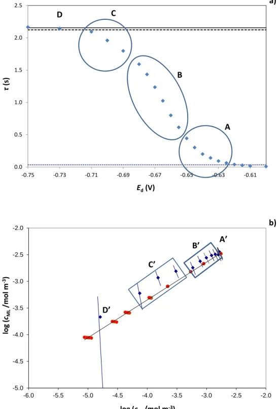
The procedure to obtain the free and bound metal at the electrode surface from each wave point was applied to the SSCP wave shown in Fig. 3a, which was carried out at 5.0×10-3 _mol·m-3 _{Cd(II) in presence of 0.0316 Kg·m}-3 _{of LFA at pH 6.0 and 10 mol·m}-3

NaNO3. The resulting cML vs. cM plot is shown in Fig. 3b. In this case, AGNES and

SSCP points practically follow a straight line of slope 0.7 (see continuous line), which might indicate that a Freundlich isotherm with such heterogeneity parameter value describes these data.

Five parameters suffice to perform the computations for a given point in the SSCP wave: the total metal concentration (which is usually known), the free metal concentration in solution (e.g. obtained independently using AGNES), the deposition half-wave potential in the system with only metal, Ed,1 2M and the transition times in

diffusion limiting conditions in presence and absence of ligand (* _and * M

 ).

The error bars in the SSCP points are obtained by applying the maximum and minimum values associated to the uncertainty of the four experimental parameters in the computation. The uncertainties are computed as follows: for the limiting transition times, we apply the 95% standard deviation (2) computed from the respective SSCP curves; for the free metal concentration, we take an estimated experimental error of ±10%; and for the metal deposition half-wave potential, we consider an uncertainty of ±0.001 V.

As an example, the error bars of figure 3 are estimated using the following uncertainties: 𝜏M∗ =3.77±0.08 s, 𝐸d,1/2,M =-0.657±0.001 V, 𝑐M∗=1.7±0.2×10-3 mol·m-3,

Going from the error estimation to the results, we observe that the 0 M

c -values obtained

from points of the foot of the wave, roughly up to  < 0.5 s (20% of the limiting transition time) –region A-, cluster around the AGNES point corresponding to the same bulk concentration at which SSCP was run. The deposition potentials and deposition time applied at the foot of the wave SSCP are indeed very similar to those of the AGNES measurement, thus yielding values quite close to the bulk equilibrium situation. The following six points –region B- lie in the intermediate range of deposition potentials and for a transition time interval of 1.6 s>  > 0.6 s (between 28 and 74% of the limiting transition time). The corresponding points in B’ are in good agreement with the measured AGNES values (in the bulk) for the two preceding metal additions, of 3.0 and 2.0×10-3 _mol·m-3_{. The next three points -in region C- approach the limiting}

transition time ( = 1.80 s, 83%;  = 1.96 s, 91% and  = 2.09 s, 97%) and their processed values in C’ are somewhat less in agreement with the AGNES measurements of 1.0 and 0.6×10-3 _mol·m-3 _{total Cd(II). In this region C’, the errors in the derivative,}

which is calculated from the experimental points, become more important, thus small uncertainties in the experimental points may provoke large differences in the computation. The last point –D-, for a deposition potential of -0.73V ( = 2.14 s, 99% of *_{), yields a D’ in good agreement with the AGNES measurements, but this is}

meaningless due to the large associated error.

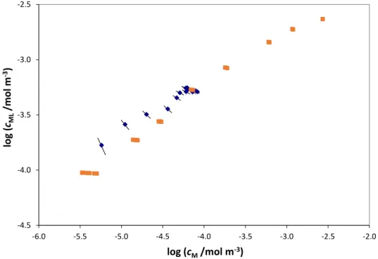
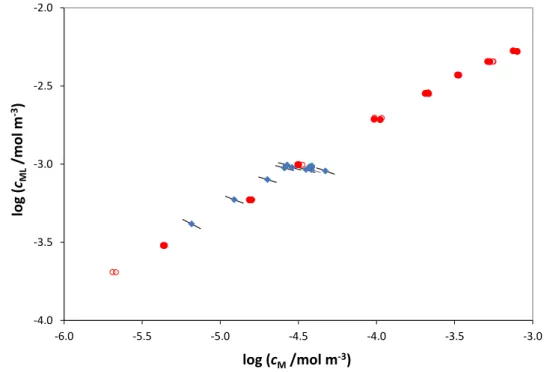
Figs. 4 and 5 depict the results obtained for the same system (Cd-LFA) at pH 7 and 8, while Figs. 6 and 7 show the results obtained for Cd binding with a purified peat humic acid at pH 6 and 7, respectively. In all these figures, the same trend can be observed: (i) a clustering of points near the initial AGNES point, (ii) a good agreement between the SSCP intermediate points and the preceding or two preceding AGNES measurements in

the bulk, and (iii) a deviation for the two or three SSCP points that are close to the limiting transition time.

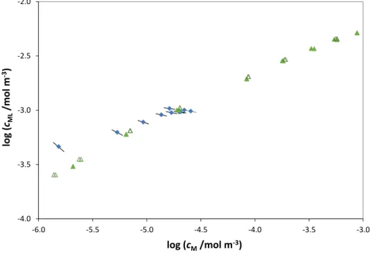
This divergence may be due to our processing already published results, since when choosing SSCP points, experimentalists tend to explore quite well the limiting transition plateau and the maximum slope region, where the half-wave potential is determined, and determine less points in the region close to the plateau since, up to now, those points were not useful. Thus, in these previous experiments there is some lack of points in the critical region C (see fig. 3), since the derivative of eqn. (31) might be more accurate with denser experimental points. Adding more SSCP points in this region will significantly improve the quality of the binding curve. This is the case in the analysis of an SSCP curve obtained for the Cd binding by fulvic acids (Fig. 8), when more points were taken in the mentioned region, yielding a better agreement between the AGNES bulk measurements and SSCP computed ones (unpublished ongoing work). As data displayed in Fig. 8 were obtained using a Screen Printed Electrode, the treatment of the results assumed mass transport by planar diffusion (i.e. using equations in ref. [14]) yielding a value of =0.53. A good agreement with AGNES measurements determined at other bulk metal concentrations is seen.

4.

Conclusions

There is a wealth of physicochemical information encapsulated in each point of an SSCP wave and its extraction is facilitated by the knowledge of the bulk free metal ion concentration determined with AGNES. With the assumptions in section 1.2 and approximating the total flux to the RDE by the sum of the individual fluxes of free metal and complex (section 1.4), one can compute: i) the normalized diffusion coefficient,  with eqn. (28), ii) the free metal ion concentration at the electrode surface

at time t=td, c_M0 , with eqn. (29) and iii) that of the complex, c_ML0 , with eqn. (31). All

these computations can be performed in a spreadsheet (like the one provided as Supporting Information). The only relevant difference between using a planar static electrode (case dealt with in ref. [14]) and the one developed here for the rotating disc electrode is the difference in the computed value of . Due to the normalizing strategy, the mathematical treatment does not require the knowledge of parameters such as deposition time, rotation speed, kinematic velocity, electrode area, number of exchanged electrons, standard redox potential, etc. The accuracy in the computation of

0 ML

c heavily depends on the determination of a derivative of the free metal ion

concentration at the surface (which is proportional to the accumulated reduced metal), so that this precision might improve with a larger number of determination and/or with special smoothing techniques, that were not used in this work. The elaboration of binding curves cML vs cM from just one SSCP wave is much faster than preparing

several solutions and apply AGNES in each of them. The reliability of a series of obtained pairs (cM, cML) at the electrode surface can be checked by running AGNES in

dedicated solutions whose bulk concentrations (cM, cML) are similar to those retrieved

from the SSCP points corresponding to potentials close to deposition under diffusion limited conditions. This opens the way to a much more time efficient work with substances such as humic and fulvic acids.

Future work will focus on the impact of loss of lability in the SSCP curve shape and how this will affect the recovery of heterogeneity information.

Acknowledgments

J.G., E.C. and J.P. gratefully acknowledge support for this research from the Spanish Ministry MINECO (Projects CTM2016-78798). L.S. Rocha and N.G. Alves produced the experimental results for the interaction of the Cd with the PSS-COOH at pH 6.5 and A. S. Costa Monteiro produced the experimental results of the Cd with the Sorocabinha fulvic acid.

References

[1] J. Buffle, Complexation Reactions in Aquatic Systems. An Analytical Approach., Ellis Horwood Limited, Chichester, 1988.

[2] H.P. van Leeuwen, J. Buffle, Chemodynamics of Aquatic Metal Complexes: From Small Ligands to Colloids, Environ. Sci. Technol. 43(19) (2009) 7175-7183.

[3] E. Rotureau, Y. Waldvogel, J.P. Pinheiro, J.P. Farinha, I. Bihannic, R.M. Present, J.F.L. Duval, Structural effects of soft nanoparticulate ligands on trace metal

complexation thermodynamics, Phys.Chem.Chem.Phys. Physical Chemistry Chemical Physics, 2016, pp. 31711-31724.

[4] J.A. Leenheer, G.K. Brown, P. MacCarthy, S.E. Cabaniss, Models of metal binding structures in fulvic acid from the Suwannee River, Georgia, Environ. Sci. Technol. 32(16) (1998) 2410-2416.

[5] H.P. van Leeuwen, R.M. Town, Stripping chronopotentiometry at scanned

deposition potential (SSCP). Part 1. Fundamental features, J. Electroanal. Chem. 536(1-2) (200536(1-2) 129-140.

[6] E. Companys, J. Galceran, J.P. Pinheiro, J. Puy, P. Salaün, A review on electrochemical methods for trace metal speciation in environmental media, Curr.Opin.Electrochem. 3(1) (2017) 144-162.

[7] A.M. Mota, J.P. Pinheiro, M.L.S. Goncalves, Electrochemical Methods for

Speciation of Trace Elements in Marine Waters. Dynamic Aspects, J. Phys. Chem. A 116(25) (2012) 6433-6442.

[8] J.P. Pinheiro, H.P. van Leeuwen, Scanned stripping chronopotentiometry of metal complexes: lability diagnosis and stability computation, J. Electroanal. Chem. 570(1) (2004) 69-75.

[9] S. Noel, J. Buffle, N. Fatin-Rouge, J. Labille, Factors affecting the flux of

macromolecular, labile, metal complexes at consuming interfaces, in water and inside agarose gel: SSCP study and environmental implications, J. Electroanal. Chem. 595(2) (2006) 125-135.

[10] R.M. Town, H.P. van Leeuwen, Dynamic speciation analysis of heterogeneous metal complexes with natural ligands by stripping chronopotentiometry at scanned deposition potential (SSCP), Aust. J. Chem. 57(10) (2004) 983-992.

[11] H.P. van Leeuwen, R.M. Town, Electrochemical metal speciation analysis of chemically heterogeneous samples: The outstanding features of stripping

chronopotentiometry at scanned deposition potential, Environ. Sci. Technol. 37(17) (2003) 3945-3952.

R.M. Town, Metal binding by heterogeneous ligands: Kinetic master curves from [12]

SSCP waves, Environ. Sci. Technol. 42(11) (2008) 4014-4021.

[13] R.F. Domingos, R. Lopez, J.P. Pinheiro, Trace metal dynamic speciation studied by scanned stripping chronopotentiometry (SSCP), Environ. Chem. 5(1) (2008) 24-32. [14] N. Serrano, J.M. Díaz-Cruz, C. Ariño, M. Esteban, J. Puy, E. Companys, J.

Galceran, J. Cecilia, Full-wave analysis of stripping chronopotentiograms at scanned deposition potential (SSCP) as a tool for heavy metal speciation: Theoretical

development and application to Cd(II)-phthalate and Cd(II)-iodide systems, J. Electroanal. Chem. 600 (2007) 275-284.

[15] W.B. Chen, C. Gueguen, D.S. Smith, J. Galceran, J. Puy, E. Companys, Metal (Pb, Cd, and Zn) Binding to Diverse Organic Matter Samples and Implications for

Speciation Modeling, Environ. Sci. Technol. 52(7) (2018) 4163-4172.

[16] E. Companys, J. Puy, J. Galceran, Humic acid complexation to Zn and Cd

determined with the new electroanalytical technique AGNES, Environ. Chem. 4 (2007) 347-354.

[17] J. Galceran, M. Lao, C. David, E. Companys, C. Rey-Castro, J. Salvador, J. Puy, The impact of electrodic adsorption on Zn, Cd or Pb speciation measurements with AGNES, J. Electroanal. Chem. 722-723 (2014) 110-118.

[18] B. Pernet-Coudrier, E. Companys, J. Galceran, M. Morey, J.M. Mouchel, J. Puy, N. Ruiz, G. Varrault, Pb-binding to various dissolved organic matter in urban aquatic systems: Key role of the most hydrophilic fraction, Geochim. Cosmochim. Acta 75(14) (2011) 4005-4019.

[19] J. Puy, J. Galceran, C. Huidobro, E. Companys, N. Samper, J.L. Garcés, F. Mas, Conditional Affinity Spectra of Pb2+_{-Humic Acid Complexation from Data Obtained}

with AGNES, Environ. Sci. Technol. 42(24) (2008) 9289-9295.

[20] R.M. Town, H.P. van Leeuwen, Stripping chronopotentiometry at scanned

deposition potential (SSCP) - Part 2. Determination of metal ion speciation parameters, J. Electroanal. Chem. 541 (2003) 51-65.

[21] J.L. Garcés, F. Mas, J. Puy, J. Galceran, J. Salvador, Use of activity coefficients for bound and free sites to describe metal-macromolecule complexation, Journal of the Chemical Society-Faraday Transactions 94 (1998) 2783-2794.

[22] J.L. Garcés, F. Mas, J. Cecília, J. Galceran, J. Salvador, J. Puy, Interpretation of speciation measurements on labile metal-macromolecular systems by voltammetric techniques, Analyst. 121(12) (1996) 1855-1861.

[23] J.L. Garcés, F. Mas, J. Cecília, J. Puy, J. Galceran, J. Salvador, Voltammetry of heterogeneous labile metal-macromolecular systems for any ligand-to-metal ratio. Part I. Approximate voltammetric expressions for the limiting current to obtain

complexation information, J. Electroanal. Chem. 484 (2000) 107-119.

[24] J.L. Garcés, F. Mas, J. Cecília, E. Companys, J. Galceran, J. Salvador, J. Puy, Complexation isotherms in metal speciation studies at trace concentration levels. Voltammetric techniques in environmental samples, PCCP 4(15) (2002) 3764-3773. [25] A.J. Bard, L.R. Faulkner, Electrochemical Methods. Fundamentals and

Applications., Second edition ed., John Wiley & Sons, Inc., New York, 2001.

[26] P.G.J. Rani, M. Kirthiga, A. Molina, E. Laborda, L. Rajendran, Analytical solution of the convection-diffusion equation for uniformly accessible rotating disk electrodes via the homotopy perturbation method, J. Electroanal. Chem. 799 (2017) 175-180. [27] V.G. Levich, Physicochemical hydrodynamics., Prentice-Hall, Englewood Cliffs,N.J., 1962.

[28] P.H.M. Leal, N.A. Leite, P.R.P. Viana, F.V.V. de Sousa, O.E. Barcia, O.R. Mattos, Numerical Analysis of the Steady-State Behavior of CE Processes in Rotating Disk Electrode Systems, J. Electrochem. Soc. 165(9) (2018) H466-H472.

[29] D. Omanovic, M. Lovric, A simulation of an anion-induced adsorption of metal ions in pseudopolarography using a thin mercury film covered rotating disk electrode, Electroanalysis 16(7) (2004) 563-571.

[30] L.S. Rocha, W.G. Botero, N.G. Alves, J.A. Moreira, A.M.R. da Costa, J.P. Pinheiro, Ligand Size Polydispersity Effect on SCCP Signal Interpretation, Electrochim. Acta 166 (2015) 395-402.

[31] N. Janot, J.P. Pinheiro, W.G. Botero, J.C. Meeussen, J.E. Groenenberg, PEST-ORCHESTRA, a tool for optimising advanced ion-binding model parameters:

derivation of NICA-Donnan model parameters for humic substances reactivity, Environ. Chem. 14(1) (2017) 31-38.

[32] W.G. Botero, M. Pineau, N. Janot, R.F. Domingos, J. Mariano, L.S. Rocha, J.E. Groenenberg, M.F. Benedetti, J.P. Pinheiro, Isolation and purification treatments change the metal-binding properties of humic acids: effect of HF/HCl treatment, Environ. Chem. 14(7) (2017) 417-424.

[33] Ecolink, Canada, Characterization of Laurentian Fulvic Acid, 1994.

[34] E.M. Thurman, R.L. Malcolm, Preparative Isolation of Aquatic Humic Substances, Environ. Sci. Technol. 15(4) (1981) 463-466.

[35] A.C.S. Monteiro, Influência da matéria orgânica natural e substâncias húmicas purificadas na especiação do Cd (II) e Pb (II) em sistemas aquáticos, PhD Thesis, UNESP, Araraquara, Brasil, 2017.

[36] S.C.C. Monterroso, H.M. Carapuca, A.C. Duarte, Performance of

poly(styrenesulfonate)-coated thin mercury film electrodes in the determination of lead and copper in estuarine water samples of high salinity, Electroanalysis 15(23-24) (2003) 1878-1883.

[37] L.S. Rocha, J.P. Pinheiro, H.M. Carapuca, Evaluation of nanometer thick mercury film electrodes for stripping chronopotentiometry, J. Electroanal. Chem. 610(1) (2007) 37-45.

[38] A.C.S. Monteiro, C. Parat, A.H. Rosa, J.P. Pinheiro, Towards field trace metal speciation using electroanalytical techniques and tangential ultrafiltration, Talanta, 2016, pp. 112-118.

[39] J. Galceran, E. Companys, J. Puy, J. Cecília, J.L. Garcés, AGNES: a new

electroanalytical technique for measuring free metal ion concentration, J. Electroanal. Chem. 566 (2004) 95-109.

[40] C. Parat, L. Authier, D. Aguilar, E. Companys, J. Puy, J. Galceran, M. Potin-Gautier, Direct determination of free metal concentration by implementing stripping chronopotentiometry as second stage of AGNES, Analyst 136 (2011) 4337-4343. [41] R.C. Weast, Handbook of Chemistry and Physics, 57 ed., CRC Press, Boca Raton, FA, 1982.

[42] B.N. Dickhaus, R. Priefer, Determination of polyelectrolyte pK(a) values using surface-to-air tension measurements, Colloid Surf. A-Physicochem. Eng. Asp. 488 (2016) 15-19.

[43] M. Filella, J. Buffle, H.P. van Leeuwen, Effect of Physicochemical Heterogeneity of Natural Complexants .1. Voltammetry of Labile Metal Fulvic Complexes,

Figures

Fig. 1: Normalized SSCP curves obtained at pH 4 and 10 mol·m-3 _{NaNO3 for 3×10}

-4 _mol·m-3 _Pb2+ _{in the calibration (+) and in presence of 4 kDa PSS-COOH polymer at}

concentrations of 5×10-2 _mol·m-3 _{(), 1×10}-1 _mol·m-3 ₍

•

4×10-1 _mol·m-3 _(). The continuous line is the average value for * _{and the dashed}

lines includes the confidence interval at 95% (2).

0.00 0.10 0.20 0.30 0.40 0.50 0.60 0.70 0.80 0.90 1.00 1.10 -0.60 -0.55 -0.50 -0.45 -0.40 τ/ τ* Ed(V)

Fig. 2: Ratios K’/cPSS obtained at each point of the SSCP curve at 10 mol·m-3 NaNO3

for (a) 3×10-4 _mol·m-3 _Cd2+ _{in presence of 10 kDa PSS-COOH at pH 4.0 (full}

symbols) and pH 6.5 (empty symbols); (b) 3×10-4 _mol·m-3 _Pb2+ _{in presence of 4}

kDa PSS-COOH polymer at pH 4.0, in presence of polymer concentrations of 5×10-2

mol·m-3 _{(), 1×10}-1 _mol·m-3 ₍

•

continuous line is the average K’/cPSS value obtained by AGNES and the dotted lines

represent the 95% confidence interval. The obtained  values in panel a) are 0.13, 0.12 and 0.11 at pH 4.0, 0.11, 0.096, 0.093, at pH 6.5, and in panel b) are 0.16, 0.14, 0.13 and 0.12, respectively. 0 50 100 150 200 250 300 350 -0.71 -0.70 -0.69 -0.68 -0.67 -0.66 -0.65 -0.64 -0.63 K'/ cPSS (m 3mol -1) E_d(V) a) 0 50 100 150 200 250 300 350 -0.52 -0.51 -0.50 -0.49 -0.48 -0.47 -0.46 -0.45 -0.44 -0.43 K'/ cPSS (m 3mol -1) E_d/V b)

Fig. 3: Bound vs. free Cd2+ _{bulk concentrations (panel b) obtained by AGNES metal}

titration from 10-4 _{to 5×10}-3 _mol·m-3 _{total Cd(II) (}

•

LFA at pH 6.0 and 10 mol·m-3 _{NaNO3 (Janot et al. [31]) and its comparison with the}

computed bound and free metal concentrations at the electrode surface () for each point of the SSCP curve (panel a) performed just for total Cd(II) 5×10-3 _mol·m -3_{. The dashed line (with slope 0.7) corresponds to the linear regression of AGNES}

points. The obtained  value is 0.21.

0.0 0.5 1.0 1.5 2.0 2.5 -0.75 -0.73 -0.71 -0.69 -0.67 -0.65 -0.63 -0.61 τ (s) Ed(V) a) -5.0 -4.5 -4.0 -3.5 -3.0 -2.5 -2.0 -6.0 -5.5 -5.0 -4.5 -4.0 -3.5 -3.0 -2.5 -2.0 log (cML /mol m -3) log (cM/mol m-3) b) A B C D A’ B’ C’ D’

Fig. 4: Bound vs. free Cd2+ _{bulk values obtained by AGNES titration from 1×10}-4 _to

5×10-3 _mol·m-3 _{total Cd(II) () in presence of 0.025 Kg·m}-3 _{of LFA at pH 7.0 and 10}

mol·m-3 _{NaNO3 (Janot et al. [31]) and its comparison with the computed bound and}

free metal concentrations at the electrode surface () for each point of the SSCP curve performed just for total Cd(II) 3×10-3 _mol·m-3. The obtained  value is 0.16.

-4.5 -4.0 -3.5 -3.0 -2.5 -2.0 -6.0 -5.5 -5.0 -4.5 -4.0 -3.5 -3.0 -2.5 -2.0 log (cML /mol m -3) log (c_M/mol m-3₎

Fig. 5: Bound vs. free Cd2+ _{bulk values obtained by AGNES titration from 1×10}-4 _to

5×10-3 _mol·m-3 _{total Cd(II) (◼) in presence of 0.010 Kg·m}-3 _{of LFA at pH 8.0 and 10}

mol·m-3 _{NaNO3 (Janot et al. [31]) and its comparison with the computed bound and}

free metal concentrations at the electrode surface () for each point of the SSCP curve performed just for total Cd(II) 6×10-4 _mol·m-3. The obtained  value is 0.36.

-4.5 -4.0 -3.5 -3.0 -2.5 -6.0 -5.5 -5.0 -4.5 -4.0 -3.5 -3.0 -2.5 -2.0 log (cML /mol m -3) log (cM/mol m-3)

Fig. 6: Bound vs. free Cd2+ _{bulk values obtained by AGNES titration from 5×10}-5 _to

6×10-3 _mol·m-3 _{total Cd(II) (}

•

mol·m--3 _{NaNO3 (Botero et al. [32]) and its comparison with the computed bound}

and free metal concentrations at the electrode surface () for each point of the SSCP curve performed just for total Cd(II) 1×10-3 _mol·m-3. The obtained  value is

0.084. -4.0 -3.5 -3.0 -2.5 -2.0 -6.0 -5.5 -5.0 -4.5 -4.0 -3.5 -3.0 log (cML /mol m -3) log (cM/mol m-3)

Fig. 7: Bound vs. free Cd2+ _{bulk values obtained by AGNES titration from 1.6×10}-4

to 6×10-3 _mol·m-3 _{total Cd(II) (, ) in presence of 0.015 Kg·m}-3 _{of HAP at pH 7.0}

and 10 mol·m-3 _{NaNO3 (Botero et al. [32]) and its comparison with the computed}

bound and free metal concentrations at the electrode surface for each point of the SSCP curve performed for total Cd(II)1×10-3 _mol·m-3_{() and 6×10}-4 _mol·m-3_().The

obtained value is 0.088. -4.0 -3.5 -3.0 -2.5 -2.0 -6.0 -5.5 -5.0 -4.5 -4.0 -3.5 -3.0 log (cML /mol m -3) log (cM/mol m-3)

Fig. 8: Bound vs. free Cd2+ _{bulk values obtained by AGNES titration from 5×10}-5 _to

2×10-3 _mol·m-3 _{total Cd(II) (}

•

acid and 10 mol·m-3 _{NaNO3 (Monteiro [35]) and its comparison with the computed}

bound and free metal concentrations at the electrode surface for each point of the SSCP curve performed for total Cd(II)2×10-4 _mol·m-3₍).  value (with the planar

diffusion treatment corresponding to a screen-printed electrode) is 0.53.

-5.0 -4.5 -4.0 -3.5 -3.0 -2.5 -6.0 -5.5 -5.0 -4.5 -4.0 -3.5 log (cML /mol m -3) log (cM/mol m-3)