Does Public Education Expansion Lead to Trickle-Down Growth?

W

ORKING

P

APERS

SES

F

S

E

S

W

-

S

F

U

F

| U

F

10.2014

N° 452

Does Public Education Expansion

Lead to Trickle-Down Growth?

Sebastian Böhm, Volker Grossmann and

Thomas M. Steger

Does Public Education Expansion Lead to

Trickle-Down Growth?

Sebastian Böhm

, Volker Grossmann

, and Thomas M. Steger

October 5, 2014

Abstract

The paper revisits the debate on trickle-down growth in view of the widely discussed evolution of the earnings and income distribution that followed a mas-sive expansion of higher education. We propose a dynamic general equilibrium model to dynamically evaluate whether economic growth triggered by an increase in public education expenditure on behalf of those with high learning ability even-tually trickles down to low-ability workers and serves them better than redistrib-utive transfers. Our results suggest that, in the shorter run, low-skilled workers lose. They are better o¤ from promoting equally sized redistributive transfers. In the longer run, however, low-skilled workers eventually bene…t more from the education policy. Interestingly, although the expansion of education leads to sustained increases in the skill premium, income inequality follows an inverted U-shaped evolution.

Key words: Directed Technological Change; Publicly Financed Education; Redistributive Transfers; Transitional Dynamics; Trickle-Down Growth.

JEL classi…cation: H20, J31, O30.

Acknowledgements: We are grateful to Sjak Smulders and Manuel Oechslin for extremely helpful comments and suggestions. We also thank seminar particants at Tilburg University, the University of Leipzig, the Humboldt University of Berlin, the "Poverty and Inequality Workshop" 2014 at Free University of Berlin, and the "70th Annual Congress of the International Institute of Public Finance (IIPF)" 2014 in Lugano for valuable discussions.

y_{University of Leipzig, Institute for Theoretical Economics, Grimmaische Strasse 12, 04109 Leipzig,} Germany, Email: boehm@wifa.uni-leipzig.de.

z_{University of Fribourg; CESifo, Munich; Institute for the Study of Labor (IZA), Bonn; Centre} for Research and Analysis of Migration (CReAM), University College London. Address: University of Fribourg, Department of Economics, Bd. de Pérolles 90, 1700 Fribourg, Switzerland. E-mail: volker.grossmann@unifr.ch.

x_{University of Leipzig; CESifo, Munich. Address: University of Leipzig, Institute for Theoretical} Economics, Grimmaische Strasse 12, 04109 Leipzig, Germany, Email: steger@wifa.uni-leipzig.de.

"Since 1979, our economy has more than doubled in size, but most of that growth has ‡owed to a fortunate few." (Barack Obama, December 4, 2013)

1

Introduction

Whether economic growth trickles down to the socially less fortunate has been a key debate for many decades in the US and elsewhere (e.g. Kuznets, 1955; Thornton, Agnello and Link, 1978; Hirsch, 1980; Aghion and Bolton, 1997; Piketty, 1997). In particular, social desirability and choices of growth-promoting policies may critically depend on their expected trickle-down e¤ects. For instance, massive expansion of high school and college education throughout the 20th century has led to a surge in the relative supply of skilled labor (Goldin and Katz, 2008; Gordon, 2013). Goldin and Katz (2008) document the important role of the public sector for this development,

particularly between 1950 and 1970.1 _{Despite steady economic growth, however,}

me-dian (full-time equivalent) earnings of males have almost stagnated from the 1970s onwards (e.g. Katz and Murphy, 1992; Acemoglu and Autor, 2012; DeNavas-Walt, Proctor and Smith, 2013). Moreover, earnings of less educated males fell considerably (Acemoglu and Autor, 2011, Tab. 1a). Thus, under the hypothesis that technological change has been endogenously skill-biased to the expansion of public education, the evidence suggests a pronounced equity-e¢ ciency trade-o¤ of this policy intervention.

In this paper, we propose a comprehensive dynamic general equilibrium framework with directed technical change, heterogenous agents and a key role of human capi-tal for economic growth to evaluate the e¤ects of public expenditure reforms on the evolution of living standards over time. In particular, we comparatively examine two public expenditure policies: public education …nance on behalf of high-ability workers and income transfers towards low-ability workers who do not acquire more advanced education (e.g. because of limited ability). We investigate whether economic growth

1_{For instance, the fraction of college students in publicly controlled institutions gradually increased} between 1900 and 1970. Between 1950 and 1970, it increased from 0.5 to almost 0.7 among students with four years of college attendance (Goldin and Katz, 2008; Fig. 7.7).

triggered by an increase in public education expenditure on behalf of those with high learning ability eventually trickles down to low-ability workers and serves them better than redistributive transfers. Relatedly, we examine whether expanding education of wealthy, high-ability households inevitably raises inequality of earnings and income over time.

Whether and when growth promoted by education expansion trickles down to low-skilled workers is a key question for at least three reasons. First, the evolution of the earnings distribution has recently provoked an intensive policy debate in the US and

elsewhere (e.g. Stiglitz, 2012; Deaton, 2013; Mankiw, 2013; Piketty, 2014).2 _For

in-stance, in his maybe most widely received speech of his US presidency (December 4, 2013), Barack Obama referred to it as "the de…ning challenge of our time",

criticiz-ing that "a trickle-down ideology became more prominent".3 _{He also urged that "we}

need to set aside the belief that government cannot do anything about reducing in-equality". In fact, the tax-transfer system in the US is rather unsuccessful to improve living standards of the working-poor, compared to other advanced countries (Gould and Wething, 2012). Second, upward social mobility has proved being severely limited by intergenerational transmission of learning ability and/or human capital, implying that a signi…cant fraction of individuals may not acquire more than basic education for

a long time to come.4 _{It is thus important to know whether those individuals pro…t}

from publicly …nanced education expansion, particularly compared to the alternative policy of redistributive transfers which are directly targeted to less educated

work-ers.5 _{To focus our analysis on this issue we deliberately rule out social mobility in}

2_{The earnings distribution has changed markedly also in Continental Europe, although later than} in the US; see e.g. Dustmann, Ludsteck and Schönberg (2009) for evidence on Germany.

3_{See www.whitehouse.gov/the-press-o¢ ce/2013/12/04/remarks-president-economic-mobility} 4_{See e.g. Corak (2013). There is overwhelming evidence for the hypothesis that the education} of parents a¤ects the human capital level of children, even when controlling for family income. For instance, Plug and Vijverberg (2003) and Black, Devereux and Salvanes (2005) show that children of high-skilled parents have a higher probability of being high-skilled.

5_{There are, of course, many other policy options to improve economic situations of the poor which} we do not consider because of our macroeconomic focus. For instance, there is a large literature on the e¤ectiveness of programmes to promote rather basic education on behalf of low-income earners or the unemployed. Some of the evidence suggests that their success is very limited unless governments intervene at a very young age (see e.g. the survey by Cunha, Heckman, Lochner and Masterov, 2006). See, however, Osikominu (2013) for qualifying evidence on long term (versus short term) active labor

our model. Third, the literature on directed technological change, initiated by Von Weizsäcker (1966) and advanced by Acemoglu (1998, 2002), suggests to account for the possibility that an increase in the supply of human capital leads to skill-biased technological change, thus contributing to the di¤erential evolution of living standards across individuals in the …rst place. Particularly, it is not evident whether and when workers with only basic education bene…t from an increase in the economy’s supply of human capital. It is therefore salient for addressing our research questions to capture the possibility that technological progress does not automatically bene…t high-skilled

and low-skilled labor in a similar fashion.6

To illustrate this point, we start out with a simple model without directed technical change where we allow for human capital externalities which bene…t both types of workers alike. We then proceed to compare the speed of trickle-down of this model to that in a comprehensive framework with R&D-based directed technical change. Standard analyses of directed technological change models are inadequate to enter the trickle-down debate, because they exclusively focus on the long run and assume that skill supply is exogenous. For instance, as acknowledged by Autor and Acemoglu (2012), such analyses are unsuccessful to explain falling earnings at the bottom of the distribution of income. Rather, our goal is to dynamically evaluate the impact of an increase in public education expenditure that potentially a¤ects both R&D and education decisions, is in line with the observed income dynamics in the last decades,

and helps to predict and understand future dynamics.7

More speci…cally, our framework rests on the following features: (i) We focus on households which do not accumulate human capital, but may bene…t from expansion

of publicly …nanced education of others either dynamically through trickle-down

market policy.

6_{In an interesting recent paper, Che and Zhang (2014) argue that the higher education expansion} in China in the late 1990s had a causal positive e¤ect on technological change particularly in human capital intensive industries, suggesting that technical change endogenously bene…ts primarily high-skilled workers.

7_{We employ the algorithm of Trimborn, Koch and Steger (2008) to analyze the transitional} dynam-ics of the resulting non-linear, highly dimensional, saddle-point stable, di¤erential-algebraic system. Despite the complexity of our model, the long run equilibrium can be derived and characterized analytically. This is important for calibrating the model and for understanding basic mechanisms.

growth or statically through complementarity of high-skilled and low-skilled labor; (ii) growth is endogenously driven by technological change which may complement di¤erent types of skills in a di¤erential fashion; (iii) the government can extend redistributive transfers and promote economic growth by publicly …nancing education; (iv) there are distortionary taxes on (labor and capital) income and capital gains; (v) the accumu-lation of physical capital, human capital and R&D-based knowledge capital interact with public policy in determining the evolution of living standards over time.

Our key …ndings may be summarized as follows. First, when the government raises the fraction of tax revenue devoted to publicly …nance education on behalf of high-ability individuals, net income and the wage rate of low-high-ability individuals …rst de-crease compared to the baseline scenario without policy reform. Thus, consistent with empirical evidence, our analysis suggests that education expansion is followed by ris-ing inequality and temporarily lower wages at the bottom of the earnris-ings distribution. Later in the transition, the economic situation of the least educated improves and they eventually become better o¤ than without education expansion. Second, an increase in the fraction of the tax revenue devoted to redistributive transfers rather than public education expenditure leads to short run gains but long run losses for this group. Thus, our analysis suggests a dynamic policy trade-o¤ from the perspective of the socially less fortunate. This is not necessarily so in the simple model without directed technical change we analyze …rst (section 3): in this model, education expansion is always inferior to transfers from the perspective of low-ability workers in the case where there are no human capital externalities; if human capital externalities are su¢ ciently strong, the picture becomes qualitatively the one suggested by the comprehensive model. Examin-ing the comprehensive model is more compellExamin-ing though for the main argument and for a quantitative analysis because it allows for the possibility that education expansion triggers technological change which primarily bene…ts high-skilled workers. Third, our calibration to the US economy implies that it takes a long time until growth triggered by education expansion trickles-down to the poor and makes them better o¤ than un-der redistributive transfers. Fourth, the speed of trickle-down is slower, the higher the (derived) elasticity of substitution between the two types of workers in the economy.

Fifth, promoting human capital accumulation implies that earnings inequality increases on impact and then further rises considerably over time. This also raises overall in-equality of net income earlier in the transition. However, although remaining higher than under redistributive transfers, income inequality eventually decreases later in the transition because of (albeit limited) convergence of asset holdings between the two types of workers. In other words, education expansion leads to an inverted U-shaped "Kuznets curve" evolution of income inequality.

The paper is organized as follows. In section 2, we brie‡y discuss the related literature. Section 3 starts out with a simple model highlighting important features of our analysis. In section 4, we set up a comprehensive growth model designed for a quantitative analysis. Section 5 characterizes its equilibrium analytically. In section 6 we employ numerical analysis to dynamically evaluate the trickle down dynamics of policy reforms. Section 7 focusses on the evolution of the distribution of earnings and net income across di¤erent types of workers. The last section concludes.

2

Related Literature

We shall not attempt to review the vast literature on the interplay between economic growth and inequality. Rather, we selectively discuss the most related work. In their seminal paper, Galor and Zeira (1993) show that human capital investments are subop-timally low under credit constraints. According to their analysis, if the wedge between the borrowing and the lending rate is su¢ ciently large, not only is inequality harmful for growth but also may it increase over time (i.e., growth does not trickle down). Aghion and Bolton (1997), Piketty (1997) and Matsuyama (2000) examine the evolution of wealth distribution under imperfect credit market with …xed investment requirements for entrepreneurial projects. They identify conditions under which growth may trickle down and argue that (lump sum) wealth redistribution to the poor may speed up this process by mitigating credit constraints. In contrast to this literature, our focus is on the interplay between physical capital accumulation, human capital accumulation and technological change directed to di¤erent types of workers, while abstracting from

credit constraints. In view of the minor role of credit constrains for education …nance in the US (for a recent study, see e.g. Lochner and Monge-Naranjo, 2011), this appears to be a reasonable research strategy in our context. Moreover, we focus on publicly …nanced education and redistribution, …nanced by distortionary taxation.

Goldin and Katz (2008) argue that the evolution of skill premia can be explained by the pace at which the relative supply of skills keeps track with the relative demand for skills as driven by skill-biased technological change. However, as already pointed out by Acemoglu and Autor (2012), their analysis does not address the possible feedback e¤ect of rising skill supply. Such e¤ects result from education expansion via endoge-nously biased technological change, altering the relative demand for skills. Closest to our analysis, Acemoglu (1998, 2002) introduces the idea that the relative demand for di¤erent types of workers via technological change is endogenous to the supply of human capital. While he focusses on the long run e¤ects of an exogenous increase in human capital, our interest lies in the transitional dynamics when both the formation of human capital and the extent and direction of technological change are endogenous to public policy reforms. Finally, Galor and Moav (2000) examine distributional e¤ects of biased technological change in a dynamic model of endogenous skill supply. There are two main di¤erences to our work. First, whereas Galor and Moav (2000) are interested in the evolution of wage inequality when the rate of (by assumption ability-biased) productivity growth starts below steady state, we evaluate public policy experiments. In particular, we consider the dynamic e¤ects of a publicly …nanced expansion of ed-ucation on behalf of high-ability individuals versus redistributive transfers on income dynamics. Second, in our model technological change is based on R&D decisions which potentially is skill-biased endogenously.

3

Simple Model

3.1

Set Up

Consider an in…nite-horizon framework in continuous time. There are two types of labor, a unit mass of type h individuals with unit time endowment, capable of accu-mulating human capital by investing time for education, and a mass l > 0 of type l individuals, inelastically supplying one unit of labor each period. For modern times, human capital accumulation of a representative type h individual may be interpreted

as higher education attendance after high school graduation.8 _{Ruling out social}

mobil-ity captures intergenerational transmission of learning abilmobil-ity in a pointed form. The modeling choice is driven by our interest of trickle-down dynamics on behalf of those (type l individuals) with basic education only.

There is a homogenous consumption good with price normalized to unity. Final output is produced under perfect competition according to

Y = Ah(HY) 1 + (LY) 1i 1 ; (1)

where HY _{and L}Y _{denote the amounts of h type and l type labor in manufacturing}

the numeraire good, A > 0 is total factor productivity, and > 0 is the elasticity of substitution between the two types of labor. Let h denote the human capital level per type h individual. We allow for a human capital externality as a channel which may a¤ect trickle-down growth; that is, A is a non-decreasing function of the human capital stock per h type individual, h; we write

A = h ,

0. In the special case = 0, there is no external e¤ect of human capital

accumula-tion on A and type l individuals are exclusively a¤ected by an increase in h because of the complementarity of di¤erent types of labor in (1). The representative …nal good

8_{In the US, secondary graduation rates increased quickly through the 20th century and then} sta-bilized (Goldin and Katz, 2008; Tab. 3.1, Fig. 6.1).

producer maximizes pro…ts, taking both A and the wage rates as given.

Skill accumulation of type h individuals depends, …rst, on the time investment in education (Lucas, 1988). Second, it depends on the amount of publicly …nanced human capital ("teachers") per type h individual devoted to educational production. Moreover, it is characterized by intergenerational human capital transmission and

de-preciation over time. Let u and 1 udenote the fraction of time a type h individual

supplies to the labor market and devotes to education, respectively. Let hE _{denote the}

teaching input in educational production per type h individual. Their human capital stock evolves according to

_h = (1 u) hE h Hh; (2)

where H > 0 is the depreciation rate of human capital and the other parameters ful…ll

> 0, _{2 (0; 1),} > 0, 0, + < 1. < 1 captures decreasing returns to

time use in education. If > 0, there is intergenerational human capital transmission.

H > 0 and + < 1 imply that, in the long run, the individual human capital level

is stationary. Suppose that the teaching input is given by9

hE = #h; (3)

where # > 0 is the fraction of human capital devoted to education. In labor market

equilibrium, uh = HY _{+ h}E_{, i.e., H}Y _{= (u #)h; moreover, L}Y _{= l.}

Our human capital accumulation process is similar to Lucas (1988), extended for

publicly provided education. Substituting (3) into (2), we …nd _h = (1 u) # h +

Hh. In Lucas (1988), = 1 (constant rather than decreasing returns to time

invest-ment), = 0(no publicly provided education), and = 1such that the stock of human

capital per capita could grow with a positive rate even in the long run, which we rule out with our parameter restrictions.

Teaching input is publicly …nanced by income taxation. In each period, a fraction

9_{In any meaningful equilibrium, the fraction must be lower than the fraction of time devoted to} labor market participation, # < u.

sE _{> 0 of contemporaneous total tax revenue is used to publicly …nance teachers} in the education sector, endogenously determining policy parameter #. Moreover, a

constant fraction sT _{> 0of the tax revenue is devoted to …nance transfers to individuals}

who own income below some income threshold, which may be thought of social welfare

expenditure; sE_+sT _{1. The possibility s}E_+sT _{< 1allows for a third public spending}

category which may additively enter the utility function (like public expenditure for defense, the legal system, public order, and safety). Alternatively, the third category may be interpreted as government waste.

Let wl denote the wage rate (and gross wage income) of type l individuals and

wh the wage rate per unit of human capital supplied by type h individuals;

supply-ing a fraction u of their unit time endowment to the labor market, their gross wage

income reads as whuh. We focus throughout on the case where type l individuals

earn (endogenously) less than type h individuals at all times. Marginal tax rates on labor income are, if anything, higher for type h individuals. Formally, suppose that the marginal income tax rate is given by an increasing step-function ~( ) ful…lling

~(whuh) h > l ~(wl). We focus on the case in which the step-function ~ is such

that h and l are time-invariant for the income ranges we consider.10 Suppose that

only type l individuals earn su¢ ciently little to be eligible for a transfer payment,

denoted by T . Their income level then reads as yl := (1 l)wl+ T, whereas after-tax

income of type h individuals is given by yh := (1 h)whuh.

Denote the level of consumption of a type j individual by cj, j 2 fh; lg. Let

subscript t on a variable index time (suppressed if not leading to confusion). As there

is no physical capital, individuals do not save, i.e. cjt = yjt for all t, j 2 fh; lg. Suppose

that intertemporal utility of a type h individual is given by

Uh = Z 1 0 (cht)1 1 1 e t_{dt =} Z 1 0 ((1 h)whtutht)1 1 1 e t_{dt. (4)}

The optimal sequence of time allocation, futg1t=0, maximizes (4) subject to (2), taking

10_{Ensuring this outcome may require that the mapping from income brackets to marginal tax rates} is adjusted when income levels grow, i.e. function ~( ) is adjusted over time.

the path of hE _{as given. The equilibrium analysis of the model proposed in this section} is standard and relegated to an online-appendix.

3.2

Policy Evaluation

We now contrast the dynamic e¤ects of an expansion of education (increase in sE₎

and of higher transfers (increase in sT_{) on income y}

l of type l individuals. For given

tax rates, an increase in sE _{raises the fraction of human capital devoted to education,}

#, whereas an increase in sT _{raises transfer payment T . Throughout the paper, we}

maintain the assumption that individuals do not anticipate shocks in policy parameters.

0 100 200 300 400 500t 1.00 1.05 1.10 1.15 1.20 yl,t yl 0 50 100 150 200 250t 1.00 1.05 1.10 1.15 1.20 1.25 yl,tyl

Plot (a): =0 Plot (b): =0.25

Figure 0: Time path of normalized income, yl=yl, in three scenarios: solid (blue) line:

baseline scenario (sT _{and s}E _{remain constant), horizontal dashed line: s}T _{increases by …ve}

percentage points), increasing dashed line: sE _{increases by …ve percentage points. Set of}

parameters: sT _{= 0:07,s}E _{= 0:1(pre-shock levels),}

h = 0:35, l = 0:17, H = 0:023,

= 0:84, = 0:25, = 0:35, = 1:5, = 0:02, = 1:91,l = 0:15. The calibration

strategy is described in appendix.

Let y_l denote the net income (and consumption) of a type-l household in initial

steady state (before the policy reform). Figure 0 illustrates the e¤ects of increases in

sE _{("education expansion") and in s}T _{("redistribution extension") by …ve percentage}

points on normalized net income yl=yl. Panel (a) treats the case without human

capital externality ( = 0). The increasing (dashed) line shows that an increase in sE

leaves low-ability workers worse o¤ early in the transition compared to the baseline scenario without policy reform. This re‡ects a reallocation of high-skilled labor away

depressing the marginal product of type l workers (decrease in @Y =@LY_{). Because} of a complementarity between both types of labor in production function (1), later

in the transition, yl rises as human capital accumulates. However, for = 0, type l

individuals turn out being worse o¤ than under the alternative policy of raising sT_,

which once and for all raises living standards of the recipients of transfer income, as indicated by the horizontal (dashed) line in panel (a). In Panel (b), we consider the same policy shocks for the case where there is a human capital externality ( = 0:25). Thus, human capital accumulation triggered by expanding education now also increases total factor productivity. Now, although living standards again drop on impact in

response to an increase in sE_{, type l individuals become better o¤ in the longer run,}

compared to the e¤ect of increasing sT_{. Comparing the results suggested by panel}

(a) and (b) of Figure 0 highlights the salient role of endogenous technological progress which we examine next in a more comprehensive way for the purpose of quantitative analysis.

4

Comprehensive Model

The model in the previous section is too simple for a quantitative policy evaluation. We next propose a comprehensive model with endogenous and directed technical change. It features may be viewed as a microfoundation of human capital externalities. Unlike in the simple model, however, education expansion does not automatically bene…t low-skilled workers through increases in total factor productivity. Its e¤ect runs through R&D investment which may be primarily directed to high-skilled intensive production. We also introduce savings and capital accumulation.

4.1

Firms

There is again a homogenous …nal good with price normalized to unity. Following Acemoglu (2002), …nal output is now produced under perfect competition according to

Y =h(XH) " 1 " + (X_L) " 1 " i " " 1 ; (5)

" > 0. XL and XH are composite intermediate inputs. They are also produced under perfect competition, combining capital goods ("machines") with human capital and low-skilled labor, respectively. Formally, we have

XH = (HX)1 AH Z 0 xH(i) di; (6) XL = (LX)1 AL Z 0 xL(i) di; (7)

0 < < 1, where xH(i) and xL(i) are inputs of machines, indexed by i, which are

complementary to the amount of human capital in this sector, HX_{, and low-skilled}

labor, LX, respectively. The mass ("number") of machines, AH and AL, expands

through horizontal innovations, as introduced below. The initial number of both types

of machines are given and positive; AH;0> 0, AL;0 > 0.

In each machine sector there is one monopoly …rm the innovator or the buyer of

a blueprint for a machine. They produce with a "one-to-one" constant-returns to scale technology by using one unit of …nal output to produce one machine unit. The total capital stock, K, in terms of the …nal good, thus reads as

K = AH Z 0 xH(i)di + AL Z 0 xL(i)di: (8)

Machine investments are …nanced by bonds sold to households. In each machine sector there is a competitive fringe which can produce a perfect substitute for an existing machine (without violating patent rights) but is less productive: input coe¢ cients are

higher than that of the incumbents by a factor _{2 (1;} 1]in both sectors.11 _Parameter

determines the setting power of …rms and allows us to disentangle the price-mark up from output elasticities, which is important for a reasonable calibration of the

model. Physical capital depreciates at rate K 0.

There is free entry into two kinds of competitive R&D sectors. In one sector, a

representative R&D …rm directs human capital to develop blueprints for new machines

used to produce the human capital intensive composite input, XH, the other sector to

produce XL. To each new idea a patent of in…nite length is awarded. Following Jones

(1995), ideas for new machines in the R&D sectors are generated according to _

AH = ~H(AH) HHA; ~H = (HHA) ; (9)

_

AL = ~L(AL) HLA; ~L= (HLA) ; (10)

where HHAand HLAdenote human capital input in the R&D sector directed to the human

capital intensive and low-skilled intensive intermediate goods sector, respectively. > 0

is a R&D productivity parameter. _{2 (0; 1) captures a negative R&D ("duplication")}

externality (Jones, 1995) which measures the gap between privately perceived constant

R&D returns of human capital and socially decreasing returns. We assume that ₂

(0; 1). > 0 captures a positive ("standing on shoulders") spillover e¤ect.12

4.2

Households

There are again two types of individuals, indexed by j 2 fl; hg, which di¤er with respect to their learning ability. The learning technology is identical to section 3: only type h individuals can accumulate human capital, according to (2). We now allow

population sizes of both types, Nh > 0 and Nl > 0, to grow at the same and constant

exponential rate, n 0. We normalize the initial size of the type h population to

unity, Nh;0 = 1, and denote Nl;0 = l. Preferences of individuals of type j 2 fl; hg are

represented by the standard utility function

Uj = 1 Z 0 (cjt)1 1 1 e ( n)t_{dt; (11)}

> 0, where cjt is consumption of a type j individual at time t.

12_{Two remarks are in order. First, Acemoglu (1998, 2002) focusses on a "lab-equipment" version} of the R&D process. Since empirically R&D costs are mainly salaries for R&D personnel, we prefer speci…cations (9) and (10). Second, < 1 implies that growth is "semi-endogenous" (Jones, 1995), i.e. would cease in the long run if we population growth were absent.

Households can hold bonds providing capital which serves as input for machine

producers, and equity thereby …nancing blueprints for machine producers. Financial

markets are always in (no-arbitrage) equilibrium. Asset holdings in per member of

dynasty j are denoted by aj. Initial asset holdings are given by ah;0 > 0, al;0 > 0.

The interest rate for bonds is denoted by r. Dividends from equity holdings and bond

holdings are taxed by the same constant rate r. Maintaining the same labor income

schedule as in section 3, assets accumulate according to

_ah = yh ch; with yh := [(1 r)r n]ah+ (1 h)whuh; (12)

_al = yl cl; with yl:= [(1 r)r n]al+ (1 l)wl+ T. (13)

yj again denotes net income of type j 2 fl; hg. Capital gains are taxed with constant

tax rate g. Again, a fraction sE of total tax revenue is devoted to publicly …nancing

education on behalf of type h individuals and a fraction sT _{…nances transfers on behalf}

of type l individuals.

5

Equilibrium Analysis

This section derives important analytical results. In section 6, we will examine whether the calibrated model implies su¢ ciently strong trickle-down e¤ects of an increase in education expenditure which eventually bene…ts the less fortunate better than extend-ing redistribution. In addition to the evolution of net income of low-ability dynasties, we also consider that of their wage rate. In section 7, we study the dynamic e¤ects of policy reforms on relative earnings and relative net income between the two types of individuals.

5.1

Preliminaries

The equilibrium de…nition is standard and relegated to the appendix. It turns out that, for the transversality conditions of household optimization problems to hold and

space such that

n + ( 1)g > 0 with g n(1 )

1 : (A1)

As will become apparent, g is the long run growth rate of individual consumption

levels, individual income components, and knowledge measures AH, AL. Thus, in

the long run, technological change turns out to be unbiased. In modern times and advanced economies, on average, the per capita income growth rate exceeds the popu-lation growth rate (g > n), implying

> : (A2)

Pro…t maximization of non-R&D producers implies two intermediate results which relate to the previous literature, reminding us on the mechanics of directed technical change.

Lemma 1. De…ne + "(1 ). The relative wage per unit of human capital

between type h and type l individuals reads as

wh wl = H X LX 1 AH AL 1 : (14)

All proofs are relegated to the appendix. According to (14), is the "derived" elasticity between high-skilled and low-skilled labor in production (Acemoglu, 2002). That is, for given productivity levels, an increase in relative amount of type h human

capital devoted to manufacturing, HX_=LX_{, by one percent reduces the relative wage}

rate, wh=wl, by 1= percent. Notably, if " > 1, then " > > 1; if " < 1, then

" < < 1.

Let PX

H and PLX denote the price of the high-skilled intensive and low-skilled

in-tensive composite intermediate good used in the …nal goods sector, respectively. An

increase in the relative knowledge stock of the high-skilled intensive sector, AH=AL,

has two counteracting e¤ects on relative wage rate as given by (14). First, the relative productivity of type h human capital in the production of composite intermediates

rises, wh=wlincreases for a given relative price of intermediates, P PHX=PLX. Second, however, since relatively more of the high-skilled intensive composite good is produced

when AH=AL rises, the relative price of composite goods, P , decreases for given labor

inputs. Through this e¤ect, the relative value of the marginal product of type h hu-man capital declines. If and only if the elasticity of substitution between the composite intermediates is su¢ ciently high, " > > 1, the …rst e¤ect dominates the second one (vice versa if " < < 1).

The next result provides insights on relative R&D incentives in the two R&D sectors. The respective pro…ts of an intermediate good …rms (symmetric within sectors) are

denoted by H and L.

Lemma 2. The relative instantaneous pro…t of machine producers reads as

H L = AH AL 1 HX LX 1 : (15)

There are counteracting e¤ects of an increase in relative employment in composite

input production, HX_=LX_{, on relative R&D incentives. First, for a given relative price}

of the high-skilled intensive good, P , relative pro…ts in the high-skilled intensive sector rise ("market size e¤ect"). Second, however, P falls in response to an increase in relative output of the high-skilled intensive good ("price e¤ect"). In the case where " > > 1, the …rst e¤ect dominates the second one, and vice versa if " < < 1.

Moreover, as already discussed after Lemma 1, an increase in the relative knowledge

stock of the high-skilled intensive sector, AH=AL, reduces the relative price P . Thus,

relative pro…ts H= L decline. The magnitude of the elasticity of H= L with respect

to AH=AL is inversely related to the "derived" elasticity between high-skilled and

5.2

Balanced Growth Equilibrium

It turns out that restricting focus on the case in which the derived elasticity of substi-tution is bounded upwards,

2

1 ; (A3)

is su¢ cient for existence and uniqueness of a balanced growth equilibrium. We focus on this case throughout. The balanced growth equilibrium is characterized by

Proposition 1. Under (A1)-(A3), there exists a unique balanced growth

equilib-rium which can be characterized as follows:

(i) ch, cl, ah, al, AH, AL, wh, wl, T grow with rate g;

(ii) LX_{, H}X_{, H}A

H, HLA, PHA, PLA grow with rate n;

(iii) XH, XL grow with rate g + n;

(iv) r, PX

H, PLX, h, u are stationary;

(v) the fraction of time a type h individual participates in the labor market is independent of policy parameters and reads as

u = n + ( 1)g + (1 ) H

n + ( 1)g + (1 + ) H

u ; (16)

(vi) the human capital level per type h individual is increasing in the fraction of human capital devoted to publicly …nanced teaching, #, and independent of other policy parameters; it reads as h = (1 u ) # H 1 1 h : (17)

According to (5), Proposition 1 implies that also per capita income grows at rate

g in steady state. The result parallels the well-known property of semi-endogenous

growth models that the economy’s growth rate is policy-independent (e.g. Jones, 1995, 2005). Interestingly, taxation and public education policy have no e¤ect on the time allocation of type h individuals (part (v) of Proposition 1). This is true even during the transition to the steady state (not shown). These result are implications of assuming time-invariant policy instruments and dynastic households.

An increase in the fraction of human capital demanded by the government for

educating type h individuals, # = hE_{=h(triggered by an increase in tax revenue share}

sE_{), raises the long run supply of human capital (part (v) of Proposition 1). However,}

if # were too high, public education expansion could lower the supply of human capital

to private …rms per type h individual, S (uh hE_{). The next result provides us}

with a condition ruling out this implausible outcome for the long run.

Corollary 1. The long run supply of human capital per type-h individual, S

(u #)h , is increasing in # if and only if

# < u

1 : (A4)

Finally, in line with empirical estimates suggesting that the elasticity of substitution between high-skilled and low-skilled labor is larger than one (Johnson, 1997), we focus on the case where

> 1: (A5)

The subsequent propositions 2 and 3 show the e¤ects of changes in tax revenue

shares sE _{and s}T _{on the steady state wage rate (and wage income) of type l individuals,}

w_l, and on the relative wage per unit of human capital between type h and type l

individuals in steady state, w_h=w_l.

Proposition 2. Under (A1)-(A5), the wage rate of type l individuals in the long

run, w_l, is increasing in sE _{(or #), and independent of s}T_.

First, recall from (17) that an increase in # raises the long run level of human capital per type h individual, h . Under (A4), in the long run, the amount of human

capital devoted to production, HX, thus rises, in turn raising the output level of the

human capital intensive composite income, XH. For given knowledge stocks, because

of the complementarity of composite inputs in …nal goods production, this raises the

price of the low-skilled labor intensive composite input, PX

L . Moreover, as discussed

in HX_=LX _{on relative pro…ts for high-skilled intensive production,}

H= L, dominates

the "price e¤ect". Thus, an increase in # spurs innovation directed to type h human

capital relatively more, i.e. AH=AL rises. As this also raises relative output XH=XL

of the composite goods, PX

L increases also through this e¤ect. As a result, the value

of the marginal product of low-skilled labor unambiguously increases in response to

expanding education. Second, an increase in sT_{, which …nances the transfer to type l}

individuals, is neutral with respect to the allocation of human capital, therefore leaving

w_l una¤ected.

Proposition 3. Under (A1)-(A5), the following holds for the relative wage per

unit of human capital between type h and type l individuals in the long run, w_h=w_l.

(i) If = 2₁ (i.e., (A3) holds with equality), w_h=w_l is independent of sE _(or

#); otherwise (if < 2₁ ), w_h=w_l is decreasing in #,

(ii) w_h=w_l is independent of sT_.

Consider an (endogenous) increase in the type h human capital for the production

of composite inputs, raising HX_=LX _{in long run equilibrium. As in models with an}

exogenous educational composition of the workforce, an increase in HX=LX could be

triggered by an increase in the supply of skilled labor. As suggested by the discussion

of Proposition 2, an increase in HX=LX could be driven by a higher fraction of human

capital demanded by the government for teaching, #. Also recall that, for > 1,

an increase in HX=LX spurs innovation directed to type h human capital relatively

more, thus raising AH=AL. According to Lemma 1, for > 1, an increase in the

"relative knowledge stock", AH=AL, would raise the relative wage rate per unit of

type h human capital, wh=wl, for given HX=LX. However, under limited (derived)

substitutability between type h and type l labor, , as assumed in (A3), the e¤ect is

not large enough to overturn the negative impact of an increase of HX_=LX _{(as triggered}

by a higher fraction of human capital demanded by the government for teaching, #)

on wh=wl for a given relative knowledge stock, AH=AL (see (14) in Lemma 1). If (A3)

6

Trickle Down Dynamics

Like in section 3, we examine the dynamic implications of two policy experiments on net income of type l individuals, i.e. an increase in the share of the total tax revenue

devoted to publicly …nanced higher education, sE, versus an equally sized increase in

the share of the total tax revenue devoted to redistributive transfers, sT_{. Moreover, we}

discuss our conclusions in several respects.

To this end, we apply the relaxation algorithm (Trimborn, Koch and Steger, 2008) which is designed to deal with highly-dimensional and non-linear di¤erential-algebraic equation systems. A favorable feature of the relaxation algorithm is that it does not rely on linearization of the underlying dynamic system. As we focus on potentially large policy shocks and long term macroeconomic dynamics, the initial deviation from the …nal steady state may be quite large. The di¤erential-algebraic system is summarized in the online-appendix.

6.1

Sketch of the Calibration Strategy

The details of the calibration strategy are laid out in the appendix. Importantly, we view a type l individual as representative for high school drop-outs and a type h individual as representing an "average" educated worker. The parameter values are based on observables for the US economy in the 2000s before the …nancial crisis 2007-2009 (including policy parameters), assuming that the US was in steady state initially

(i.e. before the considered policy shocks). Some parameters the economy’s growth

rate (g), the population growth rate (n), the mark-up factor ( ), the elasticity of

substitution between high-skilled and low-skilled labor ( ) are observed directly. The

other parameters are matched to endogenous observables like the full-time equivalent of

relative wage income of the di¤erent types of workers ("skill premium" whh=wl),

the fraction of time which type h individuals supply to the labor market (u), the capital-output ratio (K=Y ) and the interest rate (r). It turns out that the steady state values of individual asset holdings depends on its initial distribution. We therefore also calibrate the relative amount of asset holdings between the two types of households

initially, ah;0=al;0.

Parameter Value Parameter Value Parameter Value

n 0:01 0:4 g 0:1 g 0:02 " 1:83 l 0:17 1:5 K 0:04 h 0:35 0:5 H 0:03 r 0:17 0:75 1:3 sE 0:1 0:02 0:25 sT 0:07 r 0:07 0:35 # 0:04 1:91 0:25 l 0:15 0:2 0:15 ah;0=al;0 5

Table 1: Baseline set of parameters.

6.2

Expanding Education versus Extending Redistribution

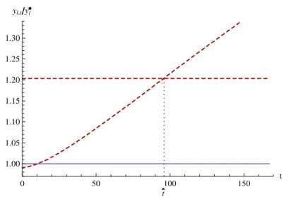
0 50 100 150 t 1.00 1.05 1.10 1.15 1.20 1.25 1.30 yl,tyl t

Figure 1: Time path of normalized income, yl=yl, in three scenarios: solid (blue) line:

baseline scenario (sT _{and s}E _{remain constant), horizontal dashed line: s}T _{increases by …ve}

percentage points), increasing dashed line: sE increases by …ve percentage points. Parameter values as in Table 1.

In Figure 1, like for the simple model, we comparatively consider the e¤ects of an

individuals, yl=yl, where superscript (*) again denotes initial steady state values. On impact, again, expanding education hurts the poor, whereas enhancing redistribution

favors the poor, as compared to the baseline scenario. An increase in sE _{diverts human}

capital (complementary to the type l workers) from manufacturing activity on

im-pact (decrease in HX_{) whereas increasing transfers leaves the human capital allocation}

una¤ected. After about 11 years, net income of low-skilled workers in the scenario "education expansion" is equated with that in the baseline scenario. Eventually, un-like in panel (a) but un-like in panel (b) of Figure 0 displaying policy responses for the simple model, growth trickles down to the poor and makes them better o¤ than under a "redistribution extension". (The mechanisms are discussed in detail in the next

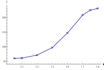
sub-section.) Denote by ^t the time span (to be interpreted as the number of years) after

a policy reform in t = 0 such that net income of low-skilled workers in the scenario "education expansion" is the same as in the scenario "redistribution extension" (and

higher for t > ^t). Figure 1 suggests that, in the US, ^t = 97.

6.3

Decomposing the E¤ects of Expanding Education

0 50 100 150 t 0.0 0.2 0.4 0.6 0.8 1.0 1.2 1.4 yl,tyl 1 r rt n al,t yl Tt yl 1 l wl,t y_l

Figure 2: The time path of normalized income,yl=yl, and its additive components whensE

increases by …ve percentage points. Parameter values as in Table 1.

To gain more insights on why the poor are better o¤ in the short run under ex-tending redistributive transfers but are better o¤ in the long run in case of expanding education, and to better understand the dynamic general equilibrium interactions, we

consider a decomposition of normalized net income of a type l household in its additive components: yl y_l = (1 l)wl y_l + [(1 r)r n] al y_l + T y_l: (18)

Assuming again that sE _{is being increased from s}E _{= 0:1 to s}E _{= 0:15, Figure 2}

displays the dynamic evolution of the three additive components as given by the

right-hand side of (18), i.e. wage income net of taxes, (1 l)wl, capital income net of taxes,

[(1 r)r n] al, and redistributive transfer, T , relative to total net income of a type l

household in the long run, y_l. Apparently, the composition of income changes only

slightly along the transition. Wage growth for type l workers and increased transfer income (which is driven by general economic growth) allows accumulation of assets.

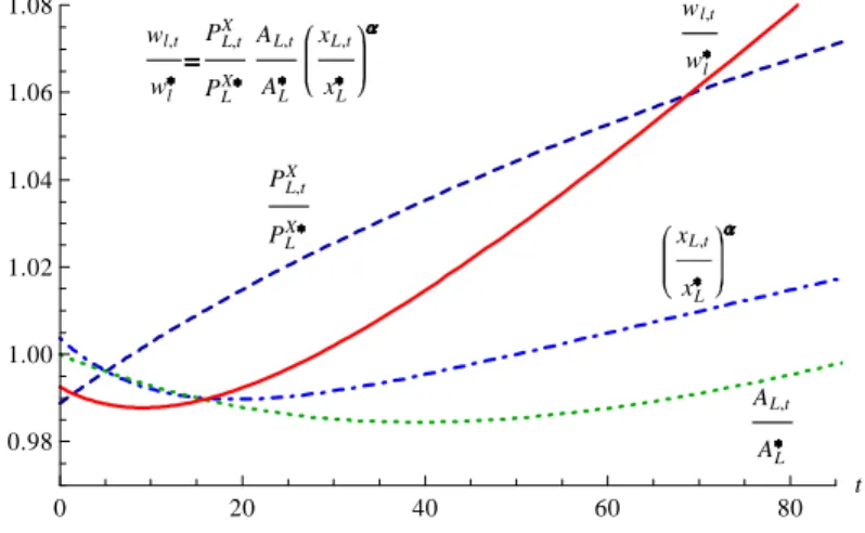
0 20 40 60 80 t 0.98 1.00 1.02 1.04 1.06 1.08 wl,t w_l PL,tX PL X AL,t A_L xL,t xL wl,t w_l P_L,tX PLX AL,t A_L xL,t x_L

Figure 3: The time path of the normalized wage rate, wl=wl, and its multiplicative

components when sE _{increases by …ve percentage points. Parameter values as in Table 1.} It is apparent that the wage component dominates the other components. Thus, we decompose the wage component further. The solid (red) curve in Figure 3 displays

the evolution of normalized wage income as given by13

wl w_l = P_LX PX L AL A_L xL x_L . (19)

13_{The wage rate (value of the marginal product) of low-ability workers may, under within-group} symmetry of machine producers, be expressed as wl = PX

L (1 ) (LX) AL(xL) (see (27) as derived in appendix).

It is driven by the three factors on the right-hand side of (19). Their evolution in

response to an increase in sE _{mirrors central human capital reallocation e¤ects. First,}

a high-ability household devotes more time to education, i.e. 1 u increases. This

implies a reduction in the total supply of skilled labor, Nhuh, on impact. Second,

an increase in sE _{allocates more skilled workers to the education sector (increase in}

teaching input hE_{). Thus, skilled labor must be initially withdrawn from production of}

the human capital intensive good and from R&D. After the initial shock, total supply

of skilled labor, Nhuh, increases because of human capital accumulation. The increased

supply is then allocated to all uses of human capital during the transition.

As a consequence, normalized wage income drops downwards initially - the solid (red) curve starts below unity - and then starts to increase monotonically. The initial

drop of wl is driven by two opposing forces. First, the price of the low-skilled labor

intensive composite (XL ) input, PLX, drops on impact in response to a reallocation

of human capital away from manufacturing. Second, the quantity of machines in this

sector, with output xL for all machine producers, goes up on impact despite the

as-sociated downward jump of price PX

L. This initial response re‡ects the e¤ect on the

interest rate r (not shown), which declines on impact, in turn reducing marginal costs of machine producers. As human capital accumulates, there is a monotonic increase of

PX

L in the aftermath of the initial drop. As discussed after Proposition 2 for the long

run, an increase in the amount of human capital used in production, HX_{, leads to a}

higher level of the human capital intensive input, XH. This pushes up the marginal

product of the low-skilled intensive composite input, therefore raising PX

L eventually.

Moreover, in the …rst phase of the transition process after an increase in sE_{, less R&D}

(directed to type l workers) is undertaken because of the reallocation of human capital

towards educational production. A decrease in HA

L depresses in turn the knowledge

stock component AL, as visualized by the downward sloping branch of the (green)

dot-ted curve. However, eventually, as more human capital becomes available, more R&D is being undertaken than initially, which eventually also bene…ts low-skilled workers.

Finally, the component (xL=xL) also follows a U-shaped evolution, partly driven by a

sector is eventually fostered, as more machine types become available (AL goes up)

and as the low-skilled intensive good becomes more expensive (PX

L rises).

In sum, the wage rate of low-skilled workers wl and therefore net income ylincrease

in the longer run in response to (i) rising prices of those goods that are produced

low-skilled labor intensively (PX

L ), (ii) a more sophisticated state of technology due to more

R&D targeted at the sector producing the low-skilled labor intensive input (raising AL),

and (iii) an accelerated accumulation of capital goods that are complementary to

low-skilled labor (xL). All of these mechanisms are fueled by the evolution of the supply

and allocation of human capital over time.

6.4

Discussion

We now discuss the trickle-down dynamics by sensitivity analysis, by looking at con-sumption rather than income, and by examining alternative ways to change public expenditure for educational and redistributive purposes. To save space, the graphs sup-porting the following arguments and extended discussions are relegated to the online-appendix.

First, in addition to the extent and direction of endogenous technical change, we suspect the trickle-down growth mechanisms to critically depend on the (derived) elas-ticity of substitution between the two types of labor.

How does a change in a¤ect the time span ^t after which type l workers are

better o¤ if the government enhances public education (increasing sE_{) compared to}

an increase in social transfers (increasing sT_{)? For a derived elasticity of substitution,}

= 1:4 (thus " = 1:67 instead of " = 1:83), type l individuals are better o¤ from

expanding education earlier than for the baseline calibration; we …nd that the threshold

time span is ^t = 71(whereas ^t = 97for = 1:5). The reason is simple: if both types of

workers are better complements, type l individuals bene…t more from human capital

accumulation. In the case where = 1:6 (i.e. " = 2), ^t rises to 147 years. Further

sensitivity analysis shows that the threshold time span ^t exists for reasonably high

and concave for high values of (see Figure A.1 in online-appendix).

Second, we may ask if the dynamic e¤ects on the consumption level of type l

individuals, cl, eventually determining their welfare, is similar to the dynamic e¤ects

on net income, yl. This is indeed the case (see Figure A.2). The initial drop in

response to an increase in sE _{is somewhat less pronounced, which re‡ects consumption}

smoothing. In the longer run, type l households eventually gain more from in increase

in sE _{than in s}T _{also in terms of consumption.}

Third, so far we have focussed on an evaluation of changing sE _{and s}T _separately,

necessarily being associated with a decrease in the government expenditure share of a third spending category. We may alternatively consider an increase (decrease) in the fraction of total tax revenue devoted to education while at the same time reducing (raising) the fraction devoted to transfers such that the sum of the two fractions,

sE _{+ s}T_{, remains constant. We …nd that, again, a policy reform towards expanding}

education is harmful in the shorter run and improves situation of type l individuals in the longer run (see Figure A.3). Moreover, extending redistribution at the expense

of education expenditure is bene…cial in the shorter run but lowers yl in the longer run

even compared to the baseline scenario without policy reform.

Fourth, so far we have left the tax rates constant and focussed on a change in

government expenditure shares, sE _{and s}T_{. What happens if we increase tax rates to}

…nance an increase in education expenditure or redistributive transfers? For instance,

suppose we increase the tax rate on bond holdings, r, to …nance an increase in transfer

T, while holding constant the government expenditure share on transfers, sT_{. The}

fraction of human capital devoted to higher education, # = hE_{=his unchanged as well.}

Such a policy reform bene…ts type l households on impact but soon becomes harmful even compared to the the baseline scenario without policy reform (see Figure A.4). The reason is the distortion of capital income taxation on savings and R&D investments by which higher transfers are …nanced. The fraction of human capital devoted to both

kinds of R&D declines, eventually depressing net income yl. Alternatively, we may

…nance an increase in # by an increase in r, while holding the education expenditure

rate g. We thus …x the growth-adjusted transfer ~T T e gt _{at its initial level for} this policy experiment. We …nd that type l households lose on impact because of the reallocation of human capital towards educational production (also displayed in Figure A.4). During the further transition, the distortion of R&D investments causes

a further decline in yl. Comparing both policies, again, expanding education is better

in the longer run and worse in the shorter run than extending redistribution.

Fifth, examining a similar comparative policy evaluation to the previous one by

raising the labor income tax rate of type h individuals, h, instead of r, suggests

qualitatively similar dynamic e¤ects than displayed in Figure 1 (see Figure A.5).

7

Inequality Dynamics

We …nally discuss the dynamic implications of policy reforms on inequality. We consider

the evolution of both the skill premium, = whh=wl, and the relative net income

between the two types of workers, yh=yl, again in response to rasing sE and sT by …ve

percentage points.

7.1

Skill Premium

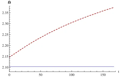
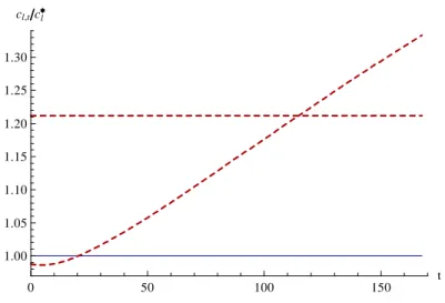
In Figure 4, the solid (blue) line displays the skill premium in the baseline scenario and

the dashed (red) line shows its evolution in response to an increase in sE_{. (The skill}

premium is una¤ected by an increase in sT_{.) Figure 4 demonstrates that expanding}

education raises earnings inequality in the short run as well as in the long run. The initial jump is driven by several reallocation e¤ects discussed above which reduce

em-ployment in the human capital intensive production sector. The drop in HX _impacts

directly on the relative wage rate, wh=wl, see (14). Thus, the relative wage rate jumps

upwards. Along the transition, the increase in earnings inequality is mainly driven by an increase in the level of human capital per type h household, h, i.e. by an increase

in human capital inequality across individuals.14 _{In the long run, is increased}

exclu-14_{In the US average years of schooling increased steadily over the period 1880 to 1980 (Goldin} and Katz, 2007, Figure 7). Rising human capital inequality as an explanation of an increasing skill

sively because of an increase in h, under the presumption of part (i) of Proposition 3, which applies for our preferred calibration.

0 50 100 150 t 2.10 2.15 2.20 2.25 2.30 2.35

Figure 4: Time path of the skill premium = whh=wl. Solid (blue) line: baseline scenario,

and increase in sT_{, increasing dashed line: s}E _{increases by …ve percentage points.}

Parameter values as in Table 1.

7.2

Income Inequality

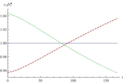
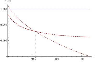
Does rising earnings inequality in response to an expansion of education imply that also inequality of net income rises over time? At the …rst glance, given that also initial asset

holdings are higher for type h individuals (ah;0 > al;0) and the long run interest rate

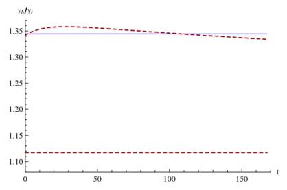
is rather high for the calibration in Table 1 (particularly, r > g), we may suspect that this is the case. Interestingly, however, Figure 5 suggests that these conditions are not

su¢ cient for relative net income between the two groups of households, yh=yl, to rise

during the entire transition in response to an increase in sE_{. Earlier in the transition}

yh=yl indeed rises, re‡ecting a rising skill premium over time. However, it turns out

that type l individuals choose their consumption path such that they accumulate assets faster than type h individuals during the entire transition (not shown); that

is, _al=al > _ah=ah. The implied (although less than full) convergence of asset holdings

eventually drives down inequality of net income even below the initial level without

premium does not, in contrast to Acemoglu (2002), require the (derived) elasticity of skilled labor and unskilled labor, , to be larger than 2.

policy reform! An increase in the fraction of tax revenue for redistributive transfers, sT_, drives down income inequality more substantially, however. Noteworthy and consistent with empirical evidence, in our calibrated model, the rich choose a higher savings rate

(not shown), i.e. _al=yl < _ah=yh.

0 50 100 150 t 1.10 1.15 1.20 1.25 1.30 1.35 yhyl

Figure 5: Time path of relative net income, yh=yl. Solid (blue) line: baseline scenario,

increasing dashed line: sT _{increases by …ve percentage points, increasing dashed line: s}E

increases by …ve percentage points. Parameter values as in Table 1.

7.3

Discussion

Comparing the e¤ects of the two considered policy options on income inequality, dis-played in Figure 5, suggests an equity-e¢ ciency trade-o¤. The dynamic, inverted U-shaped e¤ect of expanding education, suggested by Figure 5, reminds us on the famous Kuznets curve and is intriguing in itself. It contributes to the recent debate, greatly popularized by Piketty (2014), on the past and future evolution of income inequality. Our analysis suggests that income inequality may eventually go down. The result is surprising to the extent that our setup is favorable for income inequality to rise over time in response to expanding education: it features divergence in earnings with higher earnings growth rates for the initially wealthy during the entire transition. Moreover, our analysis is consistent with the evidence by Piketty (2014) and Piketty and Zucman (2014) that r > g prevails most of the time in history. Nevertheless, we have shown that these features do not allow us to draw strong conclusions on the future evolution

of the income distribution, unlike suggested by Piketty (2014). It is interesting that the decline in inequality is not just a theoretical possibility but predicted by our preferred calibration to the US economy.

8

Conclusion

The goal of this paper was to understand whether and, if yes, when economic growth caused by an increase in public education expenditure on behalf of high-ability indi-viduals trickles down to the least educated. We contrasted the dynamic e¤ects of that kind of education expansion with those of an equally sized increase in redistributive transfers. In our dynamic general equilibrium model, public expenditures are …nanced by various distortionary income taxes, human capital accumulation is endogenous, and R&D-based technical change could be directed to complement either high-skilled or low-skilled labor. In the shorter run, the poor are better o¤ from an increase in the fraction of government spending devoted to redistributive transfers and lose from ex-panding education. Consistent with empirical evidence for the US from the 1970s onwards, our analysis suggests that human capital accumulation is accompanied by falling or stagnating earnings of low-skilled individuals early in the transition phase and rising skill premia. In the longer run, however, our model predicts that low-ability workers eventually bene…t more from promoting education of high-ability workers. The time span for this to happen critically depends on the elasticity of substitution between high-skilled and low-skilled workers. The higher this elasticity is, the faster the poor bene…t from expanding education. The trickle-down e¤ect is driven by an eventual increase in the level of human capital devoted towards R&D in the sector producing low-skilled intensive goods.

Moreover, our analysis suggests that expanding education on behalf of high-ability workers triggers an inverted U-shaped evolution of income inequality. The result is remarkable in view of the prediction of a considerable and sustained increase in the skill premium, the assumption that low-ability households start with lower initial asset holdings, and an interest rate which exceeds the long run growth rate of earnings

(r > g). However, redistributive transfers are more successful in reducing inequality of net income compared to extending public education …nance.

In sum, we identi…ed two kinds of trade-o¤s regarding the alternative policies we consider which are potentially informative for the recent policy debate on income in-equality. First, there is a dynamic trade-o¤ with respect to absolute income of the poor. In the shorter run, low-ability households would always prefer higher transfers. If the goal of policy makers is, however, to improve absolute living standards of these house-holds in the longer run, promoting education of high-ability workers is more promising. Second, there is a long run trade-o¤ between the goal of raising living standards of the poor and reducing income inequality. Although both policy measures we considered lead to an eventual decline of net income dispersion, redistributive transfers are more successful in this respect.

These complex trade-o¤s call for a careful normative analysis which is left for future research. It also appears valuable to check robustness of our results in an alternative framework which highlights intergenerational con‡icts resulting from the kind of policy trade-o¤s suggested by our analysis.

Appendix

De…nition of Equilibrium (comprehensive model). Let PX

H and PLX denote the

price of the high-skilled intensive and low-skilled intensive composite intermediate good

used in the …nal goods sector, respectively, and pH(i), pL(i) the prices of machine i in

the respective composite input sector. Moreover, let PA

H and PLA denote the present

discounted value of the pro…t stream generated by an innovation in the low-skilled and high-skilled intensive sector, respectively. These are equal to equity prices. The exclusion of arbitrage possibilities in the …nancial market implies that the after-tax returns from equity (capital gains and dividends) in both sectors and bonds and must be equal; that is,

(1 g) _ P_HA PA H + (1 r) H PA H = (1 g) _ P_LA PA L + (1 r) L PA L = (1 r)r: (20)

For given policy parameters ( g; r; h; l; sE; sT), an equilibrium consists of time paths

for quantities HX

t ; LXt ; HHtA;

HA

Lt; ht; ut; hE; XHt; XLt;fxHt(i)gi_2[0;AHt];fxLt(i)gi2[0;ALt]; AHt; ALt; cht; clt; aht; alt; Ttg

and prices fPX

Ht; PLtX;fpHt(i)gi_2[0;AHt];fpLt(i)gi2[0;ALt]; P

A

Ht; PLtA; wht; wlt; rtg such that

1. R&D …rms and producers of the …nal good, the composite intermediate goods,

and machines maximize pro…ts;15

2. type h households maximize utility Uh s.t. (2) and (12); type l households

maximize Ul s.t. (13);16

3. the no-arbitrage conditions (20) in the …nancial market hold; 4. the total value of assets (owned by households) ful…lls

Nhah+ Nlal= K + PHAAH + PLAAL; (21)

where K is given by (8).

5. the labor markets for type–h and type–l workers clear:

HX + H_HA+ H_LA+ NhhE = Nhuh; (22)

LX = Nl: (23)

6. The government budgets for transfers to type l individuals (T ) and education (human capital devoted to education of type h individuals, as fraction # of the total) are balanced each period.

Proof of Lemma 1. According to (5), inverse demand functions in the composite

input sectors are given by

P_HX = @Y @XH = Y XH 1 " ; P_LX = @Y @XL = Y XL 1 " : (24)

15_{Condition 1 implies that the composite intermediate goods markets and the market for machines} clear.

16_{Households also observe standard non-negativity constraints which lead to transversality} condi-tions (see the proof of Proposition 1).

Thus, relative intermediate goods demand is given by XH XL = P X H PX L " (25)

According to (7), the inverse demand for machine i in the human capital intensive

sector is pH(i) = PHX(HX=xH(i)) 1. Machine producers, being able to transform

one unit of the …nal good to one unit of output, have marginal production costs equal

to the sum of the interest rate and the capital depreciation rate, r + K. In absence of

a competitive fringe, the incumbent’s pro…t-maximizing price would be (r + K)= . A

price equal to (r + K) (the marginal cost of the competitive fringe) is the maximal

price, however, a producer can set without losing the entire demand. Since 1= ,

it is also the optimal price. Thus, with pH(i) = pL(i) = (r + K) for all i,

xH(i) = xH = PX H (r + K) 1 1 HX =(6)_{) X}H = AHHX PX H (r + K) 1 ; (26) xL(i) = xL = PX L (r + K) 1 1 LX =(7)_{) X}L = ALLX PX L (r + K) 1 ; (27)

Hence, relative supply of composite inputs is

XH XL = AHH X ALLX PX H PX L 1 : (28)

Equating the right-hand sides of (25) and (28) and using = + "(1 )leads to

an expression for the relative price of the composite inputs,

P P X H PX L = AHH X ALLX 1 ; (29)

which is inversely related to the relative "e¢ ciency units" of high-skilled to low-skilled

labor in production activities, AHHX

ALLX .

According to (6) and (7), wage rates per unit of high-skilled and low-skilled labor are

both equations and using both (28) and (29) con…rms (14).

Proof of Lemma 2: According to (26) and (27), the instantaneous pro…ts of

machine producers, H = ( 1)(r + K)xH and L= ( 1)(r + K)xL, read as

H = ( 1) PHX 1 1 (r + K) 1 HX; (30) L= ( 1) PLX 1 1 (r + K) 1 LX: (31)

Dividing both expressions, substituting (29) and noting from the de…nition of that

1 =

"

1 con…rms (15).

Proof of Proposition 1: First, we de…ne lX _LX_=N

h, hX HX=Nh. We also

de…ne hA

k HkA=Nh, pAk PkA=Nh, k 2 fH; Lg. With these de…nitions as well as

expressions Nl=Nh = l and hE = #h from (3) we can rewrite labor market clearing

conditions (22) and (23) as

hX + hA_H + hA_L = (u #)h; (32)

lX = l: (33)

Moreover, let ~zt zte gt for z 2 fT; ch; cl; ah; al; wh; wl; Ah; Alg. That is, if a variable

z grows with rate g in the long run, then ~z is stationary. Combining (8) and (21) and

substituting both (26) and (27), we then have

~ ah+ l~al = A~H (r + K) P_HX 1 1 hX + ~ AL (r + K) P_LX 1 1 l + pA_HA~H + pALA~L: (34)

The representative R&D …rm which directs R&D e¤ort to the human capital intensive sector maximizes

P_HAA_H whHHA = P

A