Electrical Signatures of Diffusion-Limited Mixing: Insights from a Milli-fluidic Tracer Experiment
Texte intégral
Figure


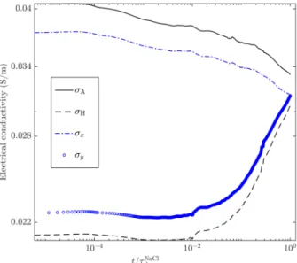
![Fig. 10 Four snapshots of the image-inferred NaCl concentration field contained in the sub-region defined by the horizontal coordinate range x ∈ [140, 175] mm at the times a t NaCl 1 = 0 , b t NaCl2 = 5 × 10 −3 , c t NaCl 3 = 5 × 10 −2 and d](https://thumb-eu.123doks.com/thumbv2/123doknet/14793473.602519/22.659.75.582.448.858/snapshots-inferred-concentration-contained-region-defined-horizontal-coordinate.webp)
Documents relatifs
[ 21 ] In summary, the deep conductivity profile obtained beneath the Western Alps in the depth range 200 – 1000 km with laboratory studies agrees with a cold mantle where water
Ainsi en est-il sur le plan artistique de l’intention de décentrement du groupe Cobra (1948-1951) qui, fondé à Paris, expose et publie au Danemark, en Belgique et aux Pays-Bas ;
In the rest of this section, first we give our results for determining duration and transition threshold, that are used for constructing mobility paths. For cell-clustering, we give
The temporal monitoring showed that for the three major crack, the alphamax index did not change with time, whereas the AAI index exhibited variations during the monitoring time. By
Alors, la vie est un labyrinthe, on analyse, on avance comme dans le labyrinthe, il y a des choix à faire, des embranchement à prendre, on a souvent la carte de ses parents.. Mais
In this study, we characterize the effects of temperature, pressure, dissolved water content and melt fraction to develop a model of electrical conductivity that can be
Training Generalization.. approach may be inconsistent when using a low number of samples and it has proposed an optimal approach based on gradient algorithm [14]. It assumes that
(The transition at TLow was not reported by them.) The small pressure dependence of TLow is in.. disagreement with the interpretation suggested
