HAL Id: halshs-01164025
https://halshs.archives-ouvertes.fr/halshs-01164025
Submitted on 16 Jun 2015
HAL is a multi-disciplinary open access
archive for the deposit and dissemination of
sci-entific research documents, whether they are
pub-L’archive ouverte pluridisciplinaire HAL, est
destinée au dépôt et à la diffusion de documents
scientifiques de niveau recherche, publiés ou non,
Insights to the European debt crisis using recurrence
quantification and network analysis
Peter Martey Addo
To cite this version:
Peter Martey Addo. Insights to the European debt crisis using recurrence quantification and network
analysis. 2015. �halshs-01164025�
Documents de Travail du
Centre d’Economie de la Sorbonne
Insights to the European debt crisis using recurrence
quantification and network analysis
Peter Martey A
DDOInsights to the European debt crisis using recurrence quantification
and network analysis
Peter Martey ADDOa,b,∗
aCentre National de la Recherche Scientifique (CNRS)
bCentre d’ ´Economie de la Sorbonne (CES) - CNRS : UMR8174 - Universit´e Paris I - Panth´eon Sorbonne, France
Abstract
The turmoil in the sovereign debt markets in Europe has raised concerns on the usefulness of sovereign credit default swaps and government bond yields in periods of distress. In addressing this issue, we introduce a novel nonlinear approach for the analysis of non-stationary multivariate data based on complex networks and recurrence analysis. We show the relevance of the approach in studying joint risk connections, extracting hidden spatial information, time dependence, de-tection of regime changes and providing early warning indicators. The feasibility and relevance of the approach in studying systemic risk is discussed. Finally, we share more light on possible extensions and applications of the approach to systemic risk.
Keywords: Sovereign debt crisis, Economic growth, Recurrence networks, Financial stability,
Systemic risk
JEL:C40, E50, G01, G18, G21
1. Introduction
The recent turmoil in the sovereign debt markets in the European Monetary Union has drawn much attention to vulnerabilities of the banking system and the whole financial system in peri-ods of distress. Some of the recent notable works documented in literature include Billio et al. (2012); Bisias et al. (2012); Acharya et al. (2013); IMF (2013); Chan-Lau et al. (2015) and the references therein. Despite ongoing economic recovery, much work still need to be done to address sovereign risks and strengthen confidence in the financial system. In this respect, our study is aimed at contributing to the prevention of crisis by highlighting policies and indica-tors that may mitigate systemic risks to enhance financial stability. This study seeks to play a role in examining the usefulness in terms of financial stability implications of government bonds and sovereign credit default swaps (SCDS) prior to and during the European debt crisis. A key concern has been whether SCDS prices provide indications of sovereign credit risk in the same fashion as the underlying government bond yields. It is unclear as to which of these market indi-cators react more rapidly to new information during periods on distress. To this date, there is still heated debate on the impact of SCDS on the stability of financial markets especially in periods
∗
Correspondence to: Centre d’ ´Economie de la Sorbonne (CES) - CNRS : UMR8174 - Universit´e Paris I - Panth´eon
Sorbonne, 106-113 boulevard de l’hopital, 75013, Paris, France.
Email address: [email protected] (Peter Martey ADDO)
of stress. In addressing issues on the usefulness of these market indicators, this paper seeks to provide evidence to assess the possible impact of some European Central Bank (ECB) policies on financial stability. In particular, this paper comments on ECB’s bond purchasing programmes and the European Union (EU) ban on purchases of naked sovereign CDS on November 1, 2012, during the debt crisis.
To address this issue, we make use of recurrence quantification analysis (RQA) (Zbilut and Webber (1992); Marwan and Kurths (2002)) and recurrence networks (Marwan et al. (2009); Donner et al. (2010)) to study the dynamics of the sovereign debt crisis across time. The RQA and recurrence networks are quantitative extensions of recurrence plots (Eckmann et al. (1987); Marwan et al. (2007); Addo et al. (2013)). These extensions are useful in examining dynamical transitions and regime change detection, the detection of phase synchronization, or the quantita-tive characterization of the dynamics of underlying time series data (see Marwan et al. (2007); Donner et al. (2011); Donges et al. (2012)). It is worth pointing out that recurrence network do not directly require knowledge about the time arrangement of observations as required by “correlation” methods such as (linear or nonlinear) autoregressive models, and mutual informa-tion models. Recurrence networks relies on the spatial structure of time series in phase space, and thus in investigating spatial dependences in the underlying process. In this paper, we pro-vide network statistics based on recurrence networks suited for identifying dynamical transitions, which can serve as systemic risk indicators or early warning measures. Aside the ability of the method to trace dynamical transitions (Donges et al. (2011)), it is applicable to non-stationary time series data. Recurrence networks allow for an intuitive and natural interpretation of results. Unlike some econometric models, recurrence networks analysis does not require stationarity or any pre-processing of the original data (Marwan et al. (2009); Donner et al. (2010)). Hence, pre-processing of the data before recurrence network analysis will depend on the researcher’s interest or the particular real-world problem considered. To our best of knowledge, this paper will serve as the first application of recurrence networks in finance and economics discipline.
This study finds some evidence that the European Monetary Union (EMU) is still in sovereign debt crisis although the government bond yields indicates signs of possible recovery in terms of reduced interest rates on government debts. Our findings suggest that the SCDS market are as useful as the government bond market in reflecting economic fundamentals and can be a useful mechanism to hedge sovereign credit risks to enhance financial stability in EMU economies. Overall, even though there is evidence of structural changes or transitions in both SCDS and government bond yields during periods of distress, it is more pronounced in sovereign CDS market. Sovereign CDS prices appear to react faster to new information via transitions than sovereign bond yields during periods of distress.
Overall, the study finds much higher interconnectedness in the EMU sovereign bond yields for observations recorded during the period of 2010–2012 marked by the European debt crisis. We also find some evidence to purport that the European Central Bank (ECB) sovereign bond purchases as interventions in debt markets under the securities markets programme (SMP) from May 2010 to September 2012 did have a positive impact on EMU yields falls. In addition, the two new purchase programmes, namely the ABS purchase programme (ABSPP) and the third covered bond purchase programme (CBPP3) announced by the ECB in September 2014 to enhance transmission of monetary policy could explain the decline in yields at the end of 2014. Our findings also suggest that the European ban on purchases of naked sovereign CDS did have negative consequences as claimed by the International Monetary Fund.
The structure of the remainder of this paper is as follows. Section 2.1 presents a description of the considered datasets used in studying the European debt crisis. Section 2.2 presents an
overview of recurrence networks, recurrence quantification analysis and complex network mea-sures useful in studying nonlinear dynamics of underlying time series data. Section 2.3 provides information on available programming packages for the implementation of the method. The em-pirical application of the method to studying the European sovereign debt crisis is then provided. Finally, in Section 3, we discuss the results and provide concluding remarks on the advantages of this approach in the area of economics and finance. In particular, we provide conclusions and policy implications based on our findings to enhance financial stability in the European Monetary Union.
2. Data & Method 2.1. Data description
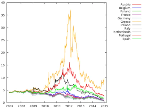
The data used in our empirical analysis consist of daily 10-year government bond yields for eleven European Monetary Union (EMU-11) countries. The EMU-11 economies used in this study is composed of the periphery group of countries: Portugal, Ireland, Italy, Greece, Spain; and the core group of countries: Austria, Germany, The Netherlands, Belgium, France, and Finland. These peripheral countries have attracted significant amount of attention from the markets and the media due to high debt levels and low levels of growth. Our choice of using the
EMU-11, which includes countries with different characteristics is to enhance a more diversified
and rich analysis of the European debt crisis. Sovereign bond yields shows how much interest a government needs to pay in order to borrow money from investors. Higher interest rate demanded by investors due to fear of failure that the governments may not be able to pay them back usually lead to what is referred to as sovereign debt crisis. The idea is to empirical investigate the EMU-11 sovereign debt crisis by examining the network dynamics of the government bond yields over
the period (01/01/2007–31/12/2014). The start date of the sample is chosen in order to study
dynamics prior and during the Sovereign debt crisis. The empirical analysis also focuses on the network dynamics of Sovereign credit default swaps (SCDS) prices for the EMU-11 economies during the European debt crisis. In this respect, we use daily data on 5-year sovereign CDS prices over the same period as the bond yields. Our daily data are sourced from Bloomberg.
2.2. Recurrence quantification& network analysis
The recurrence network analysis is a nonlinear approach based on the mix of recurrence analysis (Marwan et al. (2007); Thiel et al. (2006)) and complex network revealing temporal pat-tern of mutual recurrence of states and extracting essential information about the main dynamics of an underlying time series data (Marwan et al. (2009); Donner et al. (2010, 2011); Donges
et al. (2012)). For any given time series, denote by Xt, we can generate an embedded version in
phase space via Takens’ embedding theorem (Takens (1981)). This is achieved by first estimat-ing the embeddestimat-ing dimension and time delay (see Takens (1981); Marwan et al. (2007); Kantz and Schreiber (1997); Addo et al. (2014) and the references therein). In this work, we make use of an unembedded multivariate time series such that each time index (i) corresponds to a state
vector Xiwith components being the observation of each subprocess at that time index.
Unem-bedding the time series has its advantages when performing recurrence quantification analysis (RQA)(Thiel et al. (2006); Zbilut and Webber (1992); Marwan and Kurths (2002); Trulla et al. (1996)). The adjacency matrix of an unweighted and undirected complex network associated to the underlying time series is given by
Ai, j= Ri, j(ε) − δi, j(ε), (1)
where δi, jdenote Kronecker’s delta, ε is the recurrence threshold, subscripts i, j ∈ {1, 2, · · · , T }
are time indexes and Ri, j(·) is the recurrence matrix associated with the underlying time series
Xt. The recurrence matrix (Marwan et al. (2007)) of Xtis defined by
Ri, j(ε)= Θ(ε − kXi− Xjk), (2)
where k·k denotes a suitable distance norm (i.e. say the supremum norm), andΘ(·) is the
Heav-iside function. The threshold ε for the recurrence analysis is chosen to be equal to σ√m/10 ,
where σ is the fluctuation level in signal, m is the embedding dimension of the signal (Letellier
(2006)). Note that m = 1 implies that the time series data is unembedded. Alternatively, one
can choose the threshold in such a way, that its value corresponds to 10% of the maximum phase space diameter or such that the recurrence rate is 10% (Schinkel et al. (2008); Thiel et al. (2002); Marwan et al. (2007)). The plot of the recurrence matrix is referred to as the recurrence plot. This concept of recurrence plot has recently gained considerable attention in economics and finance (see Fabretti and Ausloos (2005); Zbilut (2005); Crowley and Schultz (2011); Addo et al. (2013, 2014), and the references therein). In this study, we will make use of measures for the quantifi-cation of recurrence plots. These measures are usually referred to as recurrence quantifiquantifi-cation analysis (RQA) developed by Zbilut and Webber (1992); Marwan and Kurths (2002); Trulla et al. (1996) and also detailed in Marwan et al. (2007). The measures include the recurrence rate (in %), determinism (in %), laminarity (in %) and the averaged diagonal line length. See Appendix A for details. These measures will be used in studying the time dependence and the detection of transitions in the dynamics of our underlying time series data. It is worth pointing out that RQA is build upon temporal structures in the form of diagonal and vertical lines, thus placing under the class of correlative-based methods of time series analysis (Zbilut and Webber (1992); Marwan and Kurths (2002)).
Unlike the wide class of methods which are based on the quantification of temporal interre-lationships between observations, recurrence networks takes into account the mutual proximity relationships of observations. The recurrence network represents the (univariate or multivariate) time series by taking into consideration the spatial information. Recurrence network provides an interpretation of the recurrence structure of a time series as a connectivity pattern of an asso-ciated complex network representation by a graph. Unlike RQA, time information is lost after transformation into a network representation. The recurrence network has been successfully used as a nonlinear approach for window-based analysis of non-stationary data and also much short time series data (say length, T ≤ 300) (Marwan et al. (2009); Donner et al. (2011)). This complex network method has been proven to be useful in identification of structural changes in the dynamics of time series (Donges et al. (2011)). For the detection of structural changes in the dynamics of the underlying time series, we make use of expanding windows and perform the subsequent analysis for the data contained in each window separately. Thus, our analysis is performed on expanding windows of the non-stationary time series and also on the full sample period considered for the study.
Complex network measures associated with recurrence networks such as transitivity
(Boc-caletti et al. (2006)), assortativity, global clustering coefficient, and average path length are
pre-sented in Appendix B and well detailed in Newman (2003); Saramaki et al. (2007); Donner et al. (2010); Donges et al. (2011); Donner et al. (2011). In general, transitivity is a measure of the regularity of the dynamics seen in the recurrence network, where higher values corresponds to regular and not chaotic dynamics. In short time series, this measure is a more robust measure
than the global clustering coefficient, which gives an overall indication of the clustering in the
network (Newman (2002); Saramaki et al. (2007); Donner et al. (2010); Donges et al. (2011)).
The assortativity measure can be interpreted as the Pearson correction coefficient between
ver-tices with a similar number of connections (ki= PjAi, j) (Newman (2002, 2003)). Other words,
it is a measure of resemblance of connections in the graph with respect to the node degree ki.
High assortativity coefficient means that connected vertices tend to have the similar assigned
values. The Average path length, L , is sensitive to dynamical transitions or structural changes in the underlying time series (Marwan et al. (2009); Donner et al. (2010)). From an economic
point of view, changes in L can be read as an indicator for regime changes and/or early warning
sign of crisis. For a comprehensive study and detailed background of the underlying analytical theory of recurrence networks, we refer the reader to Marwan et al. (2009); Donner et al. (2010, 2011); Donges et al. (2012) and the references therein.
The recurrence network analysis relies on the spatial structure of time series in phase space and does not require any time-information. Issues with strong auto-correlation are avoided by construction. This method allows a direct application to the underlying data without any trans-formation for stationarity. The properties of recurrence networks have been widely examined in Marwan et al. (2009); Donner et al. (2010, 2011) and successfully used in practice by Donges et al. (2011) in identifying dynamical transitions in marine palaeoclimate records. In this study, we will employ both the RQA and recurrence networks to capture both temporal and spatial dependences between observations in the underlying time series respectively. It is worth noting that to our best of knowledge, this is the first application of recurrence networks in economics and finance.
2.3. Implementation
In the implementation of the recurrence quantification analysis and recurrence networks, we make use of the Python programming language, and in particular the package “pyunicorn”. The Python packages “NetworkX” and “PyGraphviz” have been used for the visualization of network graphs. In particular, we make use of the Los Alamos National Laboratory (lanl) internet routes algorithm for the graphical representation of the complex networks based on the adjacency matrices defined by equation (1). For the calculation of complex network measures and related measures, the Python package “igraph” has been used.
In the section that follows, we will present the results on the application of the approach to the European Monetary Union datasets in described in Section (2.1). A discussion of the feasibility and relevance of the approach in studying systemic risk is then presented.
3. Discussion of results & implications
Our discussion begins with results on the analysis performed on the daily 10-year European sovereign bond yields. The time series plot is shown in Figure (1). In Figure (2), the recurrence plot of adjacency matrix and a graphical representation of the recurrence networks of the daily
10-year European Sovereign bond yields over the full sample period: 1/01/2007 – 31/12/2014
are displayed. Unless otherwise stated in this manuscript, the figure labels “2007” means the period from 1/01/2007–31/12/2007 and the time window with format “20AA”–“20BB” denotes the period from the start date of year “20AA” to the end date of year “20BB”. The butterfly-like structures on the diagonal of the recurrence plot in Figure (2a) can be interpreted as rare or crisis events, where the size of the “wings” of the butterfly-like structures corresponds to the impact of such an event (Addo et al. (2013, 2014)). In the context of our study, these structures corre-sponds to periods of rising bond yields in EMU-11, making it more expensive for governments
to borrow and pay their debt. In other words, these are times when investors become fearful that a government may not pay them back, leading them to often demand a higher interest rate on money to be borrowed. Figure (2b) shows a graphical representation of the recurrence network of the daily 10-year EMU-11 sovereign bond yields based on the adjacency matrix.
Figure 1: Plot of the daily 10-year European (EMU-11) Sovereign bond yields for the full sample period: 1/01/2007 –
31/12/2014.
(a) Recurrence plot of adjacency matrix. (b) Recurrence network with the Internet lanl Routes
repre-sentation
Figure 2: Recurrence Plot of the adjacency matrix associated with the recurrence network of the daily 10-year European Sovereign bond yields of the full sample period: 1/01/2007 – 31/12/2014. The time indexes in the Figure (2a) corresponds to the following dates: “1”= 1/01/2007, “500”= 11/28/2008, “1000” = 10/29/2010, “1500”= 9/28/2012, and “2000”=
8/29/2014.
(a) Betweenness (b) Closeness
(c) Degree (d) Eigenvector
Figure 3: Centrality measures based on the Recurrence network of the daily 10-year European Sovereign bond yields over the period: 2007–2014. The time indexes in the plots corresponds to the following dates: “1”= 1/01/2007, “500”=
11/28/2008, “1000” = 10/29/2010, “1500”= 9/28/2012, and “2000”= 8/29/2014.
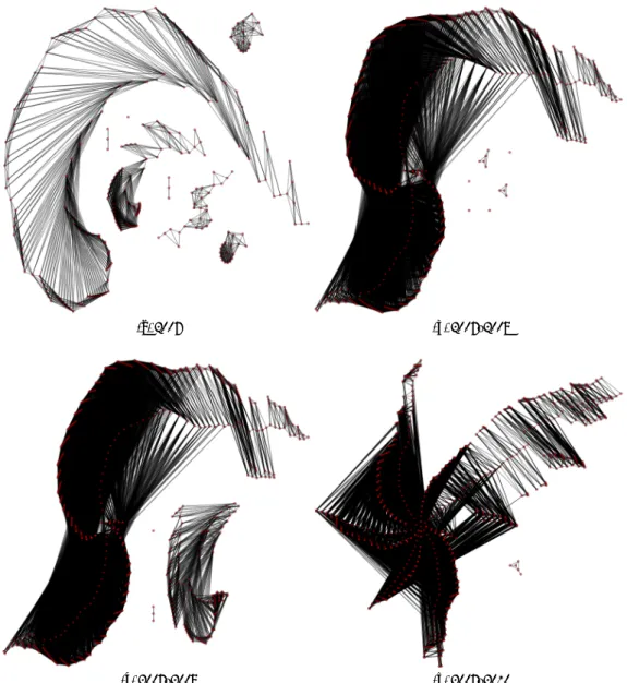
(a) 2007 (b) 2007–2008
(c) 2007–2009 (d) 2007–2010
Figure 4: Graphical representation of the recurrence network of the daily 10-year European Sovereign bond yields over
expanding windows. The year “2007” means the period from 1/01/2007–31/12/2007. The time window of the format
“20AA”–“20BB” denotes the period from the start date of year “20AA” to the end date of year “20BB”. It is important to note that in this visualization, node positions are determined by the “lanl” internet routes algorithm.
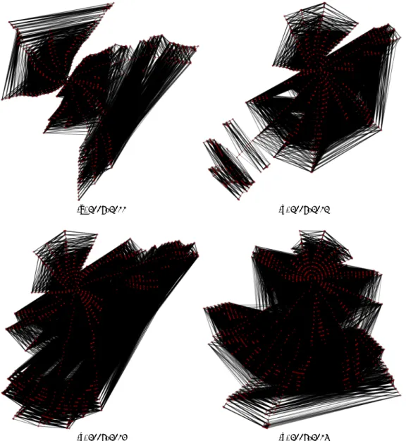
(a) 2007–2011 (b) 2007–2012
(c) 2007–2013 (d) 2007–2014
Figure 5: Graphical representation of the recurrence network of the daily 10-year European Sovereign bond yields over expanding windows. The time window of the format “20AA”–“20BB” denotes the period from the start date of year “20AA” to the end date of year “20BB”.
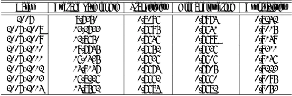
Dates Laminarity Determinism Averaged diagonal line length Recurrence rate 2007 0.6215 0.4455 2.4014 0.0479 2007–2008 0.6841 0.5375 2.5130 0.0665 2007–2009 0.6530 0.4920 2.4681 0.0508 2007–2010 0.7633 0.6169 2.6915 0.0462 2007–2011 0.8292 0.7080 3.0011 0.0511 2007–2012 0.8959 0.8183 3.7077 0.0576 2007–2013 0.9029 0.8308 3.8142 0.0506 2007–2014 0.9358 0.8903 4.7875 0.0567
Table 1: Recurrence quantification analysis (RQA) measures of the daily 10-year European Sovereign bond yields over expanding windows.
Dates Average path length Transitivity Global clustering Assortativity
2007 8.7350 0.8096 0.7974 0.8242 2007–2008 13.2733 0.7695 0.7641 0.9015 2007–2009 12.8650 0.7646 0.7688 0.9149 2007–2010 19.7745 0.7652 0.7636 0.9311 2007–2011 16.0435 0.7636 0.7606 0.9146 2007–2012 14.9147 0.7674 0.7705 0.9223 2007–2013 16.8226 0.7662 0.7660 0.9095 2007–2014 14.8562 0.7684 0.7682 0.9053
Table 2: Recurrence network measures of the daily 10-year European Sovereign bond yields over expanding windows.
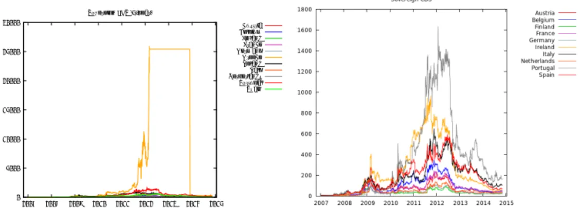
0 5000 10000 15000 20000 25000 30000 2007 2008 2009 2010 2011 2012 2013 2014 2015 Sovereign CDS (5-year) Austria Belgium Finland France Germany Greece Ireland Italy Netherlands Portugal Spain
(a) Plot of the daily 5-year European (EMU-11) CDS for the
period 1/01/2007 – 31/12/2014. (b) Plot of the daily 5-year European (EMU-11) CDS with-out Greece for the period 1/01/2007 – 31/12/2014.
(c) Recurrence plot of adjacency. (d) Recurrence network with the Internet lanl Routes
repre-sentation
Figure 6: Recurrence Plot of the adjacency matrix associated with the recurrence network of the daily 5-year European (EMU-11) Sovereign CDS for the full sample period: 1/01/2007 – 31/12/2014. The time indexes in the Figure (6c)
corresponds to the following dates: “1”= 1/01/2007, “500”= 11/28/2008, “1000” = 10/29/2010, “1500”= 9/28/2012, and
“2000”= 8/29/2014.
In order to examine the network, we present in Figure (3) centrality measures (betweenness, closeness and degree) (Freeman (1979); Donner et al. (2010)) as well as the eigenvector central-ity values associated with each vertices (i.e observation at time index) of the recurrence network shown in Figure (2b). In general, centrality measures provide information about how each ob-servation fits within the network overall. The eigenvector centrality score measures the extent to which an observation is well connected to the parts of the network with the greatest connectiv-ity. So observations with high eigenvector values seen in Figure (3d) do have many connections, and their connections have many connections in the network. The degree centrality in Figure
(3c) can be interpreted as the number of neighbors of each observation in the network. High closeness centrality observations tend to be important drivers within the network since these observations have direct links to most observations in the network. This makes the closeness centrality measure a possible indicator of crisis event since regime changes could be marked by periods of sudden rise and decline of this measure. We show in Figure (3a) the betweenness centrality which can be viewed as the number of shortest paths between pairs of observations in the network that traverse a given observation recorded at a particular time. Higher values of betweenness can be interpreted as an increase in interconnectedness in the financial system. We observe much higher interconnectedness in the daily 10-year EMU-11 Sovereign bond yields for observations recorded during the period of 2010–2012 marked by the European debt crisis. From Figure (3a), we notice that lower betweenness centrality scores are observed close to the end of year 2014, possibly providing positive indications of EMU-11 recovery from the sovereign debt crisis. In addition to the analysis performed on the complete sample period, we examine the dynamics of the network considering expanding windows. Figures (4 & 5) shows the graphical representation of the recurrence network of the daily 10-year European Sovereign bond yields over expanding windows. We can clearly observe an evolution in terms of changes in structure of the network across time. The corresponding recurrence quantification analysis (RQA) on the recurrence plot of the adjacency matrix shown in Figure (2a) are presented in Table (1). Table (2) reports results on measures based on the recurrence networks.
During the 2007–2008 financial crisis, our findings show relatively low determinism which then started raising from the beginning of the sovereign debt crisis, see Table (1). High values of laminarity, determinism and average diagonal line length were observed to increase from the period 2007–2010 to the end of 2014, providing indications of a more deterministic structure in the dynamics of the EMU-11 sovereign bond yields during the debt crisis. In general, we find relatively higher clustering and assortativity through out the recurrence networks over the consid-ered time periods, see Table (2). Dynamic transitions in terms of regime (or structural) changes are identified by looking at the changes in the average path length, L. For instance, there is a
relatively sudden change from year 2007 (L= 8.7) to 2007–2008 (L = 13.3) marking the global
financial crisis. Notice that prior to the European sovereign debt crisis, the network showed
L= 12.9, which was raised to about L = 19.8 at the beginning of the debt crisis. The decline in
this level of L as at the end of 2014 could mean that the EMU-11 is on the verge of recovery. We purport that the European Central Bank (ECB) sovereign bond purchases as interventions in debt markets under the securities markets programme (SMP) from May 2010 to September 2012 did have a positive impact on EMU-11 yields falls. In addition, the two new purchase programmes, namely the ABS purchase programme (ABSPP) and the third covered bond purchase programme (CBPP3) announced by the ECB in September 2014 to enhance transmission of monetary policy could expain the decline in L at the end of 2014.
(a) Betweenness (b) Closeness
(c) Degree (d) Eigenvector
Figure 7: Centrality measures based on the Recurrence network of daily 5-year European Sovereign CDS over the period: 2007–2014. The time indexes in the plots corresponds to the following dates: “1”= 1/01/2007, “500”= 11/28/2008,
“1000”= 10/29/2010, “1500”= 9/28/2012, and “2000”= 8/29/2014.
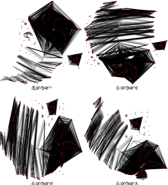
(a) 2007 (b) 2007–2008
(c) 2007–2009 (d) 2007–2010
Figure 8: Graphical representation of the recurrence network of the daily 5-year European Sovereign CDS over expanding
windows. The year “2007” means the period from 1/01/2007–31/12/2007. The time window of the format “20AA”–
“20BB” denotes the period from the start date of year “20AA” to the end date of year “20BB”.
(a) 2007–2011 (b) 2007–2012
(c) 2007–2013 (d) 2007–2014
Figure 9: Graphical representation of the recurrence network of the daily 5-year European Sovereign CDS over expanding windows. The time window of the format “20AA”–“20BB” denotes the period from the start date of year “20AA” to the end date of year “20BB”.
We now focus our discussion on the findings on the analysis performed on the EMU-11 sovereign credit default swaps (SCDS) prices. Similar to the government bond yields, we observe that the SCDS prices of peripheral countries were substantially higher than for core countries. Figure (6) shows the time series plot of the EMU-11 SCDS prices, the associated recurrence plot and recurrence network for the full sample period. Times of distress in the financial system are marked by butterfly-like structures on the diagonal of the recurrence plot displayed in Figure
Dates Laminarity Determinism Averaged diagonal line length Recurrence rate 2007 0.9524 0.9423 14.3703 0.1574 2007–2008 0.9675 0.9451 9.5813 0.1263 2007–2009 0.9705 0.9507 11.9699 0.0943 2007–2010 0.9335 0.8843 8.1657 0.0662 2007–2011 0.9316 0.8736 6.8438 0.0606 2007–2012 0.9164 0.8462 6.1775 0.0472 2007–2013 0.9229 0.8568 6.2007 0.0416 2007–2014 0.9332 0.8748 6.2158 0.0424
Table 3: Recurrence quantification analysis (RQA) measures on the daily 5-year European (EMU-11) Sovereign CDS over expanding windows.
Dates Average path length Transitivity Global clustering Assortativity
2007 1.0 1.0 0.9808 1.0 2007–2008 9.0319 0.9218 0.7841 0.9458 2007–2009 4.1777 0.8765 0.8046 0.9009 2007–2010 6.17058 0.8660 0.7941 0.9339 2007–2011 13.2437 0.8360 0.7912 0.9036 2007–2012 21.0248 0.83163 0.7903 0.9167 2007–2013 24.0126 0.8278 0.7951 0.9137 2007–2014 24.5353 0.8156 0.7924 0.8923
Table 4: Recurrence network measures on the daily 5-year European (EMU-11) Sovereign CDS over expanding windows.
(6c). The plots of centrality measures are displayed in Figure (7). The RQA results based on the
recurrence plots for different windows is reported in Table (3). The overall results shows
rela-tively higher values of laminarity and determinism in the SCDS compared to the sovereign bond yields implying that SCDS prices do not appear to be more prone to high volatility. However, the overshooting behavior in SCDS and government bond yields during periods of distress could be attributed to illiquidity in these markets. Our results provide some evidence of overshooting of SCDS prices relative to the sovereign bond markets for the EMU-11 economies during
peri-ods of stress. This claim is due to differences in the magnitude of changes in the average path
length L of the recurrence networks across expanding time windows. In particular, the changes in L in the government bond markets (see Table (2)) is lesser in magnitude relative to the SCDS (see Table (4)). This result provides indications that EMU-11 SCDS markets reacts faster to new information than in sovereign bond yields during period of crisis. However, it is unclear as to whether SCDS prices are more likely to rapidly propagate or cause contagion in other markets during periods of stress. This increase in L from the end of year 2012 (see Table (4)) could imply that the European ban on purchases of naked Sovereign CDS did have a negative consequences probably due to decline in liquidity. This finding supports concerns raised by the International Monetary Fund (IMF) on European Union’s ban on uncovered SCDS (see Chapter 2 of the global financial stability report, IMF (2013)). Our findings in Table (4) shows that transitivity, global clustering and assortativity measures were generally high for all window periods considered in this study. These recurrence network measures were much higher before the close of year 2009,
which could imply that the sovereign CDS market embeds the risks of the financial system. This explains the more evident clustering in Figure (8) compared to Figure (9).
Finally, our findings on the sovereign CDS shows that the EMU-11 is still in sovereign debt crisis although the government bond yields indicates signs of possible recovery in terms of re-duced interest rates on government debts. The empirical results presented in this work suggest that the SCDS market are as useful as the government bond market in reflecting economic fun-damentals and can be a useful mechanism to hedge sovereign credit risks to enhance financial stability in EMU-11 economies. In other words, sovereign CDS can also serve as a reliable market indicator of debt to enhance policy making. Overall, even though there is evidence of structural changes or transitions in both SCDS and government bond yields during periods of distress, it is more pronounced in sovereign CDS market. We highly recommend that the
EMU-11 governments and regulators to make efforts to improve the functioning of sovereign CDS
market to reduce the potential for possible spillovers from sovereign credit events to enhance financial stability. Based on our findings, we suggest that the ECB introduces bond purchase programmes or the so-called quantitative easing (QE) to lower yields across the eurozone, flood a lot of cash into financial markets and reverse the deflation in the eurozone.
To conclude, a direct extension of this study will be to investigate some sort of an inter-system network analysis, where measures can be developed to study the transmission of shocks from one system to another and vice versa. For instance, this could be a step in the right direction to investigate whether sovereign debt markets, say SCDS, are more likely to rapidly cause contagion in other markets prior and during financial distress.
Acknowledgement
This project has received funding from the European Union’s Seventh Framework Programme
(FP7-SSH/20072013) for research, technological development and demonstration under grant
agreement no320270 (SYRTO). This documents reflects only the author’s view. The European
Union is not liable for any use that may be made of the information contained therein.
Appendix A. Measures for the quantification of recurrence plots
We provide below an overview on RQA measures (Zbilut and Webber (1992); Marwan and Kurths (2002)), which are based on either the diagonal or vertical structures in the recurrence plots.
1. Recurrence Rate, RR, is the percentage of recurrence points in a recurrence plot. Let N
be the number of points on the phase space trajectory, and Ri, jthe recurrence matrix, then
then recurrence rate is given by
RR= 1 N2 N X i, j=1 Ri, j. (A.1)
Hence, it is a ratio of the number of recurrence states measured with respect to all possible states.
2. Determinism, DET , is the percentage of recurrence points which form diagonal lines. Otherwise, the percentage of recurrence point forming line segments parallel to the main
diagonal. Thus determinism is an indicator of the existence of a deterministic structure in the underlying time series.
DET = PN l=lminlP(l) PN i, j=1Ri, j , (A.2)
where P(l) is the distribution (histogram) of the lengths l of diagonal lines. The numerator
of equation (A.2) can be replaced byPN
i, j=1Di, jwhere
Di, j= (
1 if (Xi, Xj) and (Xi+1, Xj+1) or (Xi−1, Xj−1) are recurrent,
0 if otherwise.
3. Laminarity, LAM, is the percentage of recurrence points which form vertical lines.
LAM= PN v=vminvP(v) PN v=1vP(v) , (A.3)
where P(v) is the distribution (histogram) of the lengths v of vertical lines.
4. Averaged diagonal line length, L, is the average length of the diagonal lines.
L= PN l=lminlP(l) PN l=lminP(l) . (A.4)
Appendix B. Measures of Recurrence networks
It is important to note that centrality measures (Freeman (1979); Donner et al. (2010)) such as betweenness, closeness, degree, eigenvector centrality, and among other complex networks measures can be readily obtained by definition of a recurrence network. We present below three of such measures:
1. Transitivity coefficient is given by
T =
P
i, j,kAi, jAj,kAk,i
P
i, j,kAk,iAk, j , (B.1)
where Ai, jis the adjacency matrix of the complex network.
2. Average Path length is given by
L= Ei, j(li j), (B.2)
where Ei, j(·) denotes mean value, li j is the shortest path length between all mutual
reach-able pairs of vertices (i, j). The pair of vertices (i, j) are said to be reachreach-able if there exists at least one path connecting i and j. So equation (B.2) can be rewritten as
L= 2 N(N − 1) X i< j li j. (B.3) 3. Assortativity is defined by R= 1 L P j>ikikjAi, j− [1LPj>i12(ki+ kj)Ai, j] 2 1 L P j>i12(k 2 i + k 2 j)Ai, j− [ 1 L P j>i12(ki+ kj)Ai, j] 2, (B.4)
where ki= PjAi, j(see Donner et al. (2010)).
References
Acharya, V., Brownlees, C., Engle, R., Farazmand, F., Richardson, M., 2013. Measuring systemic risk. in Managing and Measuring Risk: Emerging Global Standards and Regulation after the Financial Crisis, Roggi-Altman (eds.), World Scientific Series in Finance, 65–98.
Addo, P. M., Billio, M., Gu´egan, D., 2013. Nonlinear dynamics and recurrence plots for detecting financial crisis. The North American Journal of Economics and Finance 26, 416–435.
Addo, P. M., Billio, M., Gu´egan, D., 2014. Turning point chronology for the euro area: A distance plot approach. OECD Journal: Journal of Business Cycle Measurement & Analysis, 1–14.
Billio, M., Getmansky, M., Lo, A. W., Pelizzon, L., 2012. Econometric measures of connectedness and systemic risk in the finance and insurance sectors. Journal of Financial Economics 104, 535–559.
Bisias, D., Flood, M., Lo, A. W., Valavanis, S., 2012. A survey of systemic risk analytics. Annual Review of Financial Economics 4, 255–296.
Boccaletti, S., Latora, V., Moreno, Y., Chavez, M., Hwang, D. U., 2006. Complex networks: structure and dynamics. Phys. Rep 424, 175–308.
Chan-Lau, J. A., Liu, E. X., Schmittmann, J. M., 2015. Equity returns in the banking sector in the wake of the great recession and the european sovereign debt crisis. Journal of Financial Stability 16, 164–172.
Crowley, P. M., Schultz, A., 2011. Measuring the intermittent synchronicity of macroeconomic growth in europe. Inter-national Journal of Bifurcation and Chaos 21 (4), 1215–1231.
Donges, J. F., Donner, R. V., Rehfeld, K., Marwan, N., Trauth, M. H., Kurths, J., 2011. Identification of dynamical transitions in marine palaeoclimate records by recurrence network analysis. Nonlinear Processes Geophysics. 18, 545–562.
Donges, J. F., Heitzig, J., Donner, R. V., Kurths, J., 2012. Analytical framework for recurrence network analysis of time series. Physical Review E: Statistical, Nonlinear, and Soft Matter Physics 85, 046105.
Donner, R. V., Small, M., Donges, J. F., Marwan, N., Zou, Y., Xiang, R., Kurths, J., 2011. Recurrence-based time series analysis by means of complex network methods. Int. J. Bifurcation Chaos 21, 1019–1046.
Donner, R. V., Zou, Y., Donges, J. F., Marwan, N., Kurths, J., 2010. Recurrence networks– a novel paradigm for nonlinear time series. New J. Physics 12, 033025.
Eckmann, J. P., Kamphorst, S. O., Ruelle, D., 1987. Recurrence plots of dynamical systems. Europhysics Letters 4 (9), 973–977.
Fabretti, A., Ausloos, M., 2005. Recurrence plot and recurrence quantification analysis techniques for detecting a critical regime. examples from financial market indices. International Journal of Modern Physics C 16 (5), 671–706. Freeman, L., 1979. Centrality in social networks conceptual clarification. Social Networks 1, 215–239.
IMF, April 2013. Global financial stability report: Old risks, new challenges. Tech. rep., Washington: International Monetary Fund.
Kantz, H., Schreiber, T., 1997. Nonlinear Time Series Analysis. Cambridge: Cambridge University Press.
Letellier, C., 2006. Estimating the shannon entropy: recurrence plots versus symbolic dynamics. Physical Review Letters, 96:254102.
Marwan, N., Donges, J. F., Zou, Y., , Donner, R. V., Kurths, J., 2009. Complex network approach for recurrence analysis of time series. Phys. Letters A 373, 4246–4254.
Marwan, N., Kurths, J., 2002. Nonlinear analysis of bivariate data with cross recurrence plots. Physics Letters A 302 (5-6), 299–307.
Marwan, N., Romano, M. C., Thiel, M., Kurths, J., 2007. Recurrence plots for the analysis of complex systems. Physics Reports 438 (5–6), 237–329.
Newman, M. E. J., 2002. Assortative mixing in networks. Phys. Rev. Letters 89, 208701.
Newman, M. E. J., 2003. The structure and function of complex networks. SIAM Rev 45 (2), 167–256.
Saramaki, J., Kivela, M., Onnela, J. P., Kaski, K., Kert´esz, J., 2007. Generalizations of the clustering coefficient to weighted complex network. Physical Review E 75, 027105.
Schinkel, S., Dimigen, O., Marwan, N., 2008. Selection of recurrence threshold for signal detection. European Physical Journal-Special Topics 164 (1), 45–53.
Takens, F., 1981. Detecting strange attractors in turbulence. Lecture notes in mathematics, 366–387.
Thiel, M., Romano, M. C., Kurths, J., 2006. Spurious structures in recurrence plots induced by embedding. Nonlinear Dynamics 44, 299–305.
Thiel, M., Romano, M. C., Kurths, J., Meucci, R., Allaria, E., Arecchi, F. T., 2002. Influence of observational noise on the recurrence quantification analysis. Physica D 17 (3), 138–152.
Trulla, L. L., Giuliani, A., Zbilut, J. P., Webber, C. L. J., 1996. Recurrence quantification analysis of the logistic equation with transients. Physics Letters A 223 (4), 255–260.
Zbilut, J. P., 2005. Use of recurrence quantification analysis in economic time series. In: New Economic Windows: Economics Complex Windows, Eds.: M. Salzano and A. Kirman, Springer, 91–104.
Zbilut, J. P., Webber, J. C. L., 1992. Embeddings and delays as derived from quantification of recurrence plots. Physics Letters A (171), 199–203.