HAL Id: hal-00330328
https://hal.archives-ouvertes.fr/hal-00330328
Submitted on 15 Oct 2007
HAL is a multi-disciplinary open access
archive for the deposit and dissemination of
sci-entific research documents, whether they are
pub-lished or not. The documents may come from
teaching and research institutions in France or
abroad, or from public or private research centers.
L’archive ouverte pluridisciplinaire HAL, est
destinée au dépôt et à la diffusion de documents
scientifiques de niveau recherche, publiés ou non,
émanant des établissements d’enseignement et de
recherche français ou étrangers, des laboratoires
publics ou privés.
organic carbon concentration in the eastern South
Pacific
C. Grob, O. Ulloa, Hervé Claustre, Y. Huot, G. Alarcón, D. Marie
To cite this version:
C. Grob, O. Ulloa, Hervé Claustre, Y. Huot, G. Alarcón, et al.. Contribution of picoplankton to the
total particulate organic carbon concentration in the eastern South Pacific. Biogeosciences, European
Geosciences Union, 2007, 4 (5), pp.837-852. �hal-00330328�
www.biogeosciences.net/4/837/2007/ © Author(s) 2007. This work is licensed under a Creative Commons License.
Biogeosciences
Contribution of picoplankton to the total particulate organic carbon
concentration in the eastern South Pacific
C. Grob1,2,3, O. Ulloa2, H. Claustre3, Y. Huot3, G. Alarc´on2, and D. Marie4
1Graduate Programme in Oceanography, Universidad de Concepci´on, Concepci´on, Chile
2Department of Oceanography and Center for Oceanographic Research in the eastern South Pacific, Universidad de
Concepci´on, Casilla 160-C, Concepci´on, Chile
3CNRS, Laboratoire d’oc´eanographie de Villefranche, 06230 Villefranche-sur-Mer, France; Universit´e Pierre et Marie
Curie-Paris 6, Laboratoire d’oc´eanographie de Villefranche, 06230 Villefranche-sur-Mer, France
4Station Biologique, CNRS, INSU et Universit´e Pierre et Marie Curie, 29482 Roscoff Ceder, France
Received: 27 February 2007 – Published in Biogeosciences Discuss.: 9 May 2007 Revised: 6 August 2007 – Accepted: 1 October 2007 – Published: 15 October 2007
Abstract. Prochlorococcus, Synechococcus, picophy-toeukaryotes and bacterioplankton abundances and contribu-tions to the total particulate organic carbon concentration, derived from the total particle beam attenuation coefficient (cp), were determined across the eastern South Pacific
be-tween the Marquesas Islands and the coast of Chile. All flow cytometrically derived abundances decreased towards the hyper-oligotrophic centre of the gyre and were highest at the coast, except for Prochlorococcus, which was not de-tected under eutrophic conditions. Temperature and nutri-ent availability appeared important in modulating picophyto-plankton abundance, according to the prevailing trophic con-ditions. Although the non-vegetal particles tended to domi-nate the cpsignal everywhere along the transect (50 to 83%),
this dominance seemed to weaken from oligo- to eutrophic conditions, the contributions by vegetal and non-vegetal par-ticles being about equal under mature upwelling conditions. Spatial variability in the vegetal compartment was more im-portant than the non-vegetal one in shaping the water col-umn particle beam attenuation coefficient. Spatial variabil-ity in picophytoplankton biomass could be traced by changes in both total chlorophyll a (i.e. mono + divinyl chlorophyll
a) concentration and cp. Finally, picophytoeukaryotes
con-tributed ∼38% on average to the total integrated phytoplank-ton carbon biomass or vegetal attenuation signal along the transect, as determined by size measurements (i.e. equiva-lent spherical diameter) on cells sorted by flow cytometry and optical theory. Although there are some uncertainties
as-Correspondence to: C. Grob ([email protected])
sociated with these estimates, the new approach used in this work further supports the idea that picophytoeukaryotes play a dominant role in carbon cycling in the upper open ocean, even under hyper-oligotrophic conditions.
1 Introduction
Global estimates indicate that about half of the Earth’s pri-mary production (PP) takes place in the ocean (Field et al., 1998). Of a mean global marine PP of 50.7 Gt C y−1 estimated through ocean-colour-based models (Carr et al., 2006), 86% would occur in the open ocean (Chen et al., 2003). Here the photosynthetic biomass is dominated by three main picophytoplanktonic (<2–3 µm) groups (e.g. Li, 1995): cyanobacteria of the genera Prochlorococcus (Chisholm et al., 1988) and Synechococcus (Waterbury et al., 1979), and eukaryotes belonging to diverse taxa (Moon-van der Staay et al., 2001).
Although cyanobacteria, especially Prochlorococcus (Li and Wood, 1988; Chisholm et al., 1988), tend to dominate in terms of numerical abundance, it has been shown that eu-karyotic phytoplankton (usually <3.4 µm) dominates the ul-traplankton (<5 µm) photosynthetic biomass in the northern Sargasso Sea (Li et al., 1992) and in the eastern Mediter-ranean Sea (Li et al., 1993). Across the North and South Atlantic Subtropical Gyres (Zubkov et al., 1998, 2000) and eastern South Pacific (Grob et al., 2007) picophytoeukary-otes also constituted a considerable fraction of the picophy-toplanktonic carbon biomass.
Using flow cytometry cell sorting combined with14C mea-surements, Li (1994) made the only simultaneous group-specific primary production rates measurements available so far in the literature for Prochlorococcus, Synechococcus and picophytoeukaryotes. Even though he could only apply this methodology at three different stations in the North Atlantic Ocean and at a single depth per station, this author’s results showed that picophytoeukaryotes contribution to picophyto-plankton primary production increased as the Prochlorococ-cus to picophytoeukrayotes abundances ratio decreased. At a coastal Pacific site in the Southern California Bight, on the other hand, Worden et al. (2004) reported that picophy-toeukaryotes had the highest picophytoplankton growth rates and contributions to the net community production and car-bon biomass on annual bases.
Picophytoeukaryotes can therefore make a significant con-tribution to the picophytoplanktonic PP and carbon biomass (see above). Carbon being the universal currency in marine ecological modelling, looking inside the pico-autotrophic “black box” to determine the distribution of carbon biomass among the different groups becomes fundamental to better understand the respective role of these groups in the global carbon cycle. Recent biogeochemical models have made a significant step forward on this subject by incorporating not only different plankton functional types, but also differ-ent groups within these functional types (e.g. cyanobacteria, picophytoeukaryotes, nitrogen fixers) in order to reproduce some of the ecosystem’s variability (e.g. Bisset et al., 1999; Le Qu´er´e et al., 2005). Different picophytoplanktonic groups have different physiological characteristics such as optimal specific rates of photosynthesis, adaptation to light, pho-tosynthetic efficiencies and maximum specific growth rates (Veldhuis et al., 2005, and references therein). Knowing where one group dominates over the others could therefore help choosing the appropriate physiological parameters to estimate PP from surface chlorophyll a concentrations re-trieved from space and improve such estimates at the large scale.
The measurement of the particle beam attenuation coef-ficient (cp) has proven to be a very powerful tool in
deter-mining particle load and particulate organic carbon (POC) concentrations at the global (e.g. Gardner, 2006) as well as at the regional scale (e.g. Claustre et al., 1999; Oubelkheir et al., 2005). High frequency measurements of cpsignal can
also be used to derive rates of change in particulate organic stocks like gross and net community production (Claustre et al., 2007). In situ cp profiles associated with the
si-multaneous cytometric determination of the different phyto-planktonic groups and bacterioplankton (Bacteria + Archaea) abundances have the potential to allow the estimation of the contribution of these groups to the bulk cp, and hence to
POC. Group-specific contributions to POC can therefore be estimated from their contributions to cp. In the equatorial
Pa-cific, for instance, picophytoeukaryotic cells would dominate the vegetal contribution to cp (Chung et al., 1996; DuRand
and Olson, 1996; Claustre et al., 1999). These estimations require however that the mean cell size and refractive index of each group are known or at least assumed (Claustre et al., 1999, and references therein). Total and group-specific beam attenuation coefficients can be obtained at relatively short time scales, but also have the advantage of being amenable to large scale in situ surveys on carbon stocks and cycling, and even to global estimation, since bulk oceanic bio-optical properties can be retrieved from space (e.g. Gardner, 2006).
In the present work we tried to answer the following ques-tions: (1) What is the contribution of the different picoplank-tonic groups to POC in the upper ocean? and (2) How does the spatial variability in these group’s contributions influence the spatial changes in POC in the upper ocean? For this, we studied the waters of the eastern South Pacific, which present an extreme gradient in trophic conditions, from the hyper-oligotrophic waters of the central gyre to the eutrophic coastal upwelling waters off South America. Using flow cy-tometry cell sorting we were able to isolate different pico-phytoplankton populations in situ to obtain their mean cell sizes (as equivalent spherical diameters), which allowed us to improve estimations on the group-specific attenuation coeffi-cients, and therefore on group-specific contributions to POC.
2 Methods
A total of 24 stations were sampled between the Mar-quesas Islands (∼8.4◦S; 141.2◦W) and the coast of Chile (∼34.6◦S; 72.4◦W) during the French expedition BIOSOPE (BIogeochemistry and Optics SOuth Pacific Experiment) in austral spring time (26 October to 11 December 2004) (Fig. 1). Temperature, salinity and oxygen profiles were obtained with a conductivity-temperature-depth-oxygen pro-filer (CTDO, Seabird 911 Plus). Nutrient concentrations (ni-trate, nitrite, ammonium, phosphate and silicate) were de-termined onboard (see Raimbault et al., 2007). Pigment concentrations from noon profiles (local time) were de-termined using High Performance Liquid Chromatography (HPLC). For HPLC analyses, water samples were vacuum filtered through 25 mm diameter and 0.7 µm porosity What-man GF/F glass fibre filters (see Ras et al., 2007), where on average 97% of Prochlorococcus cells are retained (Chavez et al., 1995). The above implies a maximum error of 3% on the total divinyl-chlorophyll a concentrations (dv-chla, pig-ment that is specific only to this group) determined using this technique. Daily integrated surface total irradiance was de-termined from on-board calibrated measurements.
All stations reported here were sampled at local noon time at 6 to 14 different depths from the surface down to 300 m (Fig. 1). The position of the deepest sampling depth was es-tablished relative to the position of the bottom of the photic layer, Ze (m) defined as the depth where the irradiance is reduced to 1% of its surface value. Five stations of very dif-ferent trophic conditions, here referred to as long stations,
Longitude (ºW) Latitude (ºS) 72oW 90oW 108oW 144oW 126oW X 2 1 HNL MAR 44oS 36oS 28oS 4oS 12oS 20oS GYR W 5 21 20 4 19 3 17 18 6 7 8 11 12 13 1415 EGY 40oN 80oW 120oW 160oW 120oE 160oE 0o 20oS 40oS 20oN 40oN 80oW 120oW 160oW 120oE 160oE 0o 20oS 40oS 20oN
Fig. 1. BIOSOPE transect. In this study we include data from
sta-tions 1–8, 11–15 and 17–21, MAR, HNL, GYR, EGY, UPW (W) and UPX (X).
were also sampled at high frequency (i.e. every 3 h) during 2 to 4 days: (1) mesotrophic (MAR, Marquesas Islands), (2) high nutrient-low chlorophyll (HNL, ∼9.0◦S and 136.9◦W), (3) hyper-oligotrophic (GYR, ∼26.0◦S and 114.0◦W), (4) oligotrophic (EGY, ∼31.8◦S and 91.5◦W) and (5) eutrophic (UPW, highly productive upwelling region, ∼34.0◦S and 73.3◦W) (Fig. 1). The coastal-most station (UPX) was addi-tionally sampled to compare it with UPW’s upwelling condi-tion (Fig. 1).
Our results are presented in terms of oligo-, meso- and eu-trophic conditions according to surface total chlorophyll a concentrations (Tchla, chlorophyll a + divinyl chlorophyll
a) of ≤0.1, >0.1 and ≤1, and >1 mg m−3, respectively (An-toine et al., 1996). This division has been used to characterize the trophic status of the ocean from space and we consider it as appropriate to describe the large spatial patterns investi-gated during the BIOSOPE cruise.
2.1 Picoplankton analyses
Prochlorococcus, Synechococcus and picophytoeukaryotes abundances were determined on fresh samples on board with a FACSCalibur (Becton Dickinson) flow cytometer. For bac-terioplankton counts (Bacteria + Archaea), samples fixed either with paraformaldehyde at 1% or glutaraldehyde at 0.1% final concentration and quick-frozen in liquid nitro-gen were stained with SYBR-Green I (Molecular Probes) and run in the same flow cytometer within two months af-ter the end of the cruise. Reference beads (Fluoresbrite YG Microspheres, calibration grade 1.00 µm, Polysciences, Inc) were added to each sample before acquiring the data with the Cell Quest Pro software (Becton Dickinson) in logarith-mic mode (256 channels). During data acquisition, between 5×10³and 300×103events were registered in order to count at least 500 cells for each picoplanktonic group. The er-ror associated with abundances determined using flow cy-tometry is ≤5% (D. Marie, unpublished data). The data
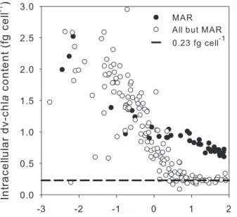
Fig. 2. Prochlorococcus intracellular dv-chla content (fg cell−1) as a function of the percentage of surface irradiance at MAR (filled circles) and the rest of the transect (empty circles). Dashed line in-dicates the average surface intracellular dv-chla content established at 0.23 fg cell−1.
were then analysed with the Cytowin software (Vaulot, 1989) to separate the picoplanktonic populations based on their scattering and fluorescence signals, according to Marie et al. (2000) (see Supp. Mat.: www.biogeosciences.net/4/837/ 2007/bg-4-837-2007-supplement.pdf).
Surface Prochlorococcus abundance for weakly fluores-cent populations (i.e. ∼7% of total samples) was estimated by fitting a Gaussian curve to the data using Cytowin. When their fluorescence was too dim to fit the curve (e.g. sur-face and sub-sursur-face samples at the center of the gyre) their abundance was estimated from dv-chla concentrations by assuming an intracellular pigment content of 0.23 fg cell−1 (see Supp. Mat.). This intracellular dv-chla content corre-sponds to the mean value obtained for cells in the surface layer (above ∼5% of surface light) by dividing the HPLC-determined dv-chla by the cell number estimated from flow cytometry, considering all but the MAR data (Fig. 2). At the GYR station, Synechococcus and picophytoeukaryotes abun-dances above 100 m were only available for the first morning profile (samples taken above 90 m for the other GYR pro-files are unfortunately not available). This profile showed that both groups’ abundances were homogeneous over the first 100 m, so we assumed the abundances measured at 90– 100 m to be representative of the abundances within the 0– 100 m layer. All picoplankton abundances were then inte-grated from the surface to 1.5 Ze rather than to Ze, because deep chlorophyll maxima (DCM) were observed between these two depths at the center of the gyre.
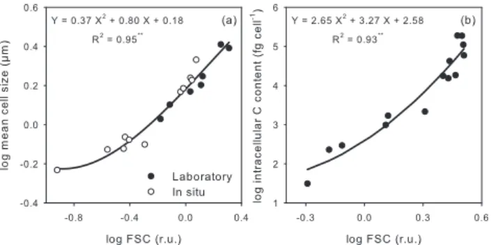
Fig. 3. Log-log relationships established between the flow
cyto-metric forward scatter signal (FSC), expressed in units relative to reference beads (relative units, r.u.), and mean cell size in µm (a) and intracellular carbon (C) content in fig cell−1(b). In (a), mean
cell sizes measured on natural populations isolated in situ (empty circles) as well as on populations from culture (filled circles) are included. Mean intracellular carbon contents in (b) were obtained from culture cells. Carbon measurements were performed on tripli-cate with ≤5% of standard deviation.∗∗indicates p<0.0001.
In order to establish a relationship between ac-tual sizes (i.e. mean cell sizes acac-tually measured) and the mean forward scatter cytometric signal normal-ized to the reference beads (FSC in relative units, r.u.; see Supp. Mat.: www.biogeosciences.net/4/837/2007/ bg-4-837-2007-supplement.pdf), in situ Prochlorococcus, Synechococcus and picophytoeukaryotes populations were sorted separately on board with a FACS Aria flow cytometer (Becton Dickinson). Each sorted population was then anal-ysed with a Multisizer 3 Coulter Counter (Beckman Coulter) for size (µm) and with the FACS Calibur flow cytometer for FSC. Several Synechococcus and picophytoeukaryotes pop-ulations isolated in situ could be measured with the Coul-ter CounCoul-ter. Prochlorococcus size, on the other hand, could only be determined for one population because they were at the detection limit of the instrument. A similar analysis was performed on monospecific cultures of various picophy-toplankton species (without pre-sorting) to combine both in situ and laboratory measurements to establish a log-log poly-nomial relationship between FSC and size (Fig. 3a). We be-lieve that even though the left-most end of the fitted curve is driven by a sole data point, it is still very useful to the re-lationship because it represents the actual mean cell size of a natural Prochlorococcus population (i.e. 0.59 µm), corre-sponding to a mean FSC of 0.02 r.u. Based on this relation-ship established within the picophytoplankton size range, we calculated the upper size limit for the FSC settings we used during the whole cruise at 3 µm (i.e. FSC=0.88 r.u.).
Also using culture cells, we established a direct relation-ship between the mean cytometric FSC signal and intracel-lular carbon content to estimate Synechococcus and pico-phytoeukaryotes carbon biomass (Fig. 3b). To obtain in-tracellular carbon contents, a known volume of each
cul-ture population was filtered onto GF/F filters previously pre-combusted at 400◦C, in triplicate. One blank filter per cul-ture was put aside to be used as control. The number of phytoplankton and contaminating bacterioplankton cells re-tained in and passing through the filters were determined us-ing flow cytometry (see Supp. Mat.: www.biogeosciences. net/4/837/2007/bg-4-837-2007-supplement.pdf). The filters were then dried at 60◦C for 24 h, fumigated with concen-trated chlorhydric acid for 6 to 8 h to remove inorganic carbon and dried again for 6 to 8 h. Each filter was fi-nally put in a tin capsule and analysed with a Carbon-Hydrogen-Nitrogen (CHN) autoanalyzer (Thermo Finnigan, Flash EA 1112) (see Supp. Mat.: www.biogeosciences.net/4/ 837/2007/bg-4-837-2007-supplement.pdf). Carbon contents were estimated based on a calibration curve performed using Acetanilide.
Considering both size and carbon content derived from FSC, a conversion factor (in fgC µm−3) was established for Synechococcus and then applied to the mean cell size esti-mated for Prochlorococcus to obtain the intracellular carbon content of that group. Picophytoplankton carbon biomass was then calculated by multiplying cell abundance and in-tracellular carbon content for each group.
2.2 Beam attenuation coefficients specific for each pi-coplankton group
Profiles of the total particle beam attenuation coefficient at 660 nm (cp, m−1), a proxy for POC (e.g. Claustre et al.,
1999), were obtained with a C-Star transmissometer (Wet Labs, Inc.) attached to the CTD rosette. Procedures for data treatment and validation have been described elsewhere (Loisel and Morel, 1998; Claustre et al., 1999). Inherent optical properties of sea water (IOP’s), such as cp, depend
exclusively on the medium and the different substances in it (Preisendorfer, 1961). The vegetal (cveg) and non-vegetal
(cnveg) contribution (Eq. 1) to the particle beam attenuation
coefficient can therefore be expressed as
cp=cveg+cnveg (1)
whereas the Prochlorococcus (cproc), Synechococcus (csyn),
picophytoeukaryotes (ceuk) and larger phytoplankton
(>3 µm, clarge) contribution to the vegetal signal (Eq. 2) can
be described by
cveg=cproc+csyn+ceuk+clarge (2)
Bacterioplankton (cbact), heterotrophs (chet) and detritus (cdet
= non living particles) contribute to the non-vegetal compo-nent (Eq. 3) as follows,
cnveg=cp−cveg
=cbact+chet+cdet
=cbact+2cbact+cdet
where chetis assumed to be approximately 2cbact(Morel and
Ahn, 1991). This assumption was adopted in order to be able to estimate the fraction of total particulate organic car-bon corresponding to detritus, which is the group of particles contributing to cpthat is not directly measured, i.e. the
unac-counted cp(see below; Eq. 4).
Since particulate absorption is negligible at 660 nm (Loisel and Morel, 1998), beam attenuation and scattering are equiv-alent, so we can estimate cproc, csyn, ceuk, clarge and cbact
by determining the group-specific scattering coefficients bi (m−1)=Ni [si Qbi], where i = proc, syn, euk, large or bact. We used flow cytometry to retrieve both picophy-toplankton cell abundance (Ni, cells m−3) and mean cell sizes (through FSC, see Sect. 2.1). Mean geometrical cross sections (s, m2 cell−1) were calculated from size, while
Qbi (660), the optical efficiency factors (dimensionless), were computed through the anomalous diffraction approx-imation (Van de Hulst, 1957) assuming a refractive in-dex of 1.05 for all groups (Claustre et al., 1999). For Prochlorococcus and Synechococcus we used mean sizes ob-tained from a few samples, whereas for the picophytoeukary-otes we used the mean cell size estimated for each sam-ple (see Supp. Mat.: www.biogeosciences.net/4/837/2007/ bg-4-837-2007-supplement.pdf). For samples where pico-phytoeukaryotes abundance was too low to determine their size we used the nearest sample value, i.e. the mean cell size estimated for the sample taken immediately above or below the missing one. This approximation was applied to ∼26% of the samples and although it may seem a large fraction, it cor-responds mostly to deep samples where cell abundance was very low. Low cell abundances will result in low biomasses and it is therefore unlikely that the error associated with this approximation will introduce important errors in the carbon biomass estimates. For bacterioplankton we used a value of 0.5 µm, as used by Claustre et al. (1999). Finally, once cveg,
cbact and therefore chet are determined, cdet is obtained
di-rectly by difference (Eq. 4).
cdet=cnveg−cbact−chet
=cnveg−cbact−2cbact
=cnveg−3cbact (4)
Contributions to cp by larger phytoplanktonic cells in
the western and eastern part of the transect were es-timated by assuming that peaks larger than 3 µm in the particle size distribution data obtained either with the Coulter Counter or with a HIAC optical counter (Royco; Pacific Scientific) corresponded to autotrophic or-ganisms (see Supp. Mat.: www.biogeosciences.net/4/837/ 2007/bg-4-837-2007-supplement.pdf). Coulter Counter data were only available for 1 (surface samples, ≤5 m) to 3 dif-ferent depths. Thus, in order to obtain water column pro-files for MAR, HNL, EGY and UPW, the estimated clarge
were extrapolated by assuming clarge=0 at the depth where
no peak >3 µm was detected (usually below 50 m). When
only surface data were available, clarge was assumed to be
negligible at the depth where chlorophyll fluorescence be-came lower than the surface one. Group-specific attenuation signals were integrated from the surface down to 1.5 Ze (wa-ter column, c0−1.5 Ze) and from the surface to 50 m (surface
layer, c0−50 m) to estimate their contribution to integrated cp.
Finally, cp(660) was converted to particulate organic
car-bon (POC) by using the empirical relationship established by Claustre et al. (1999) for the tropical Pacific (Eq. 5), which has proven to be valid as part of BIOSOPE (see Stramski et al., 2007).
POC (mg m−3)=cp(m−1) × 500 (mg m−2) (5)
Through the above relationship cpexplains ∼92% of the
vari-ance in POC concentration (Claustre et al., 1999). To eval-uate the ability of Tchla and cp to trace spatial changes in
picophytoplankton biomass along the transect, we used local noon time data within the integration depth (0 to 1.5 Ze) from the stations where no large phytoplankton cells were detected with the particle counters (Coulter or HIAC), i.e. stations 3 to 15+GYR. We chose these stations because we do not have intracellular carbon content data for larger cells to include in the photosynthetic carbon biomass estimates.
3 Results
The sampled transect included South Pacific Tropical Wa-ters (SPTW), with a clear salinity maximum extending from the surface down to 150 m between HNL and GYR, East-ern South Pacific Central Waters (ESPCW) characterized by salinities of 34.5 to 36 (Fig. 4a) and temperatures of 15 to 20◦C at the centre of the gyre (GYR to EGY) and colder and fresher waters at the Chilean coast (Claustre et al., 2007). Limits between oligo-, meso- and eutrophic conditions were set at 133, 89 and 74.5◦W according to the measured sur-face chlorophyll a concentrations, as explained above. Un-der oligotrophic conditions nitrate concentrations were close to 0 µM or undetectable between the surface and 150–200 m, and still very low (∼2.5 µM) between the latter depth and 1.5 Ze (Fig. 4b). Expectedly, nutrient concentrations were higher under mesotrophic conditions and highest near the coast (see Raimbault et al., 2007), whereas phosphate was never a limiting factor (Moutin et al., 2007).
The hyper-oligotrophic centre of the South Pacific Sub-tropical Gyre (SPSG), i.e. the clearest waters of the world’s ocean (Morel et al., 2007), was characterized by extremely low surface Tchla concentrations (<0.03 mg m−3; see Ras et al., 2007) and undetectable nutrient levels (see Raimbault et al., 2007), greatly differing from the Marquesas Islands’ mesotrophic conditions and the typical High Nutrient – Low Chlorophyll situation (i.e. HNL) encountered at the borders of the gyre, and the upwelling conditions observed at the coast.
Salinity
Nitrate concentration ( -1)
µmol L
Total particle beam attenuation coefficient (m )-1
Total chlorophyllaconcentration (mg m )-3
Depth (db) Depth (db ) Depth (db) Depth (db) Longitude (ºW) M O M E (a) (b) (d) (c)
Prochlorococcus abundance (x 10 cells ml )3 -1
Synechococcus abundance (x 10 cells ml )3 -1
Picophytoeukaryotes abundance (x 10 cells ml )3 -1
Bacterioplankton abundance (x 10 cells ml )3 -1
Longitude (ºW) Depth (db ) Depth (db) Depth (db) Depth (db) M O M E (e) (f) (g) (h)
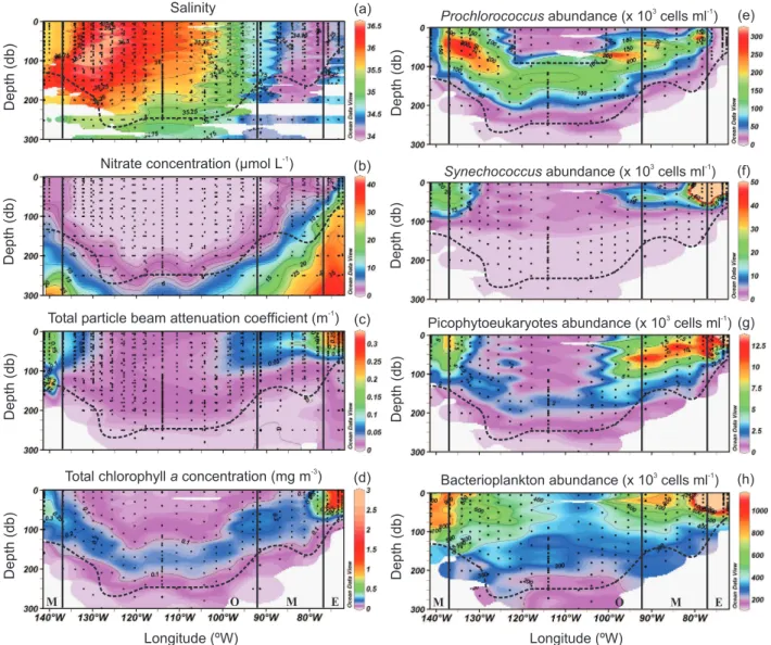
Fig. 4. Salinity (a), nitrate concentration in µmol L−1(b), total particle beam attenuation coefficient in m−1(c), total chlorophyll a
concen-tration in mg m−3(d) Prochlorococcus (e), Synechococcus (f), picophytoeukaryotes (g) and bacterioplankton (h) abundances (×103cells ml−1). Vertical black lines indicate from left to right the limits between meso- (M), oligo- (O), meso- (M) and eutrophic (E) conditions. Horizontal black dashed line corresponds to the depth of the 1.5 Ze. Black dashed square in (e) indicates where Prochlorococcus abundances were estimated from dv-chla concentration.
3.1 Picoplankton numerical abundance
All groups’ abundances tended to decrease towards the centre of the gyre. Prochlorococcus was highest at the western (up to 300×103cells ml−1around 50 m, associated with SPTW)
and eastern (up to 200×103 cells ml−1 in the 50 to 100 m
layer) borders of the oligotrophic region (Fig. 4e). Peaks in Synechococcus (up to 190×103 cells ml−1; Fig. 4f), pico-phytoeukaryotes (10–70×103cells ml−1; Fig. 4g) and bac-terioplankton abundances (up to 2×10⁶cells ml−1; Fig. 4h) were registered near the coast. Deep Prochlorococcus (100–150×103cells ml−1between 50 and 200 m; Fig. 4e) and picophytoeukaryotes (∼2×10³cells ml−1between 150
and 200 m; Fig. 4g) maxima were recorded at the centre of the gyre following the pattern of Tchla concentrations (∼0.15 mg m−3; Fig. 4d), above the deep chlorophyll
maxi-mum (DCM) for the former and within the DCM depth range for the latter (Figs. 4e and g). Synechococcus reached lower depth ranges than the rest of the groups everywhere along the transect (Fig. 4f). In terms of chlorophyll biomass, the im-portance of the DCM at the centre of the gyre is highlighted when comparing the surface-to-DCM average ratios for the different long stations: 0.67±0.13 at MAR, 0.44±0.04 at HNL, 0.12±0.02 at GYR and 0.27±0.02 at EGY.
Water column integrated picoplankton abundance (0 to 1.5 Ze) was strongly dominated by bacterioplankton along
Fig. 5. Prochlorococcus (a), and bacterioplankton (b) integrated
abundances (0 to 1.5 Ze, ×1011 cells m−2) as a function of
sur-face temperature, which was representative of the general eastward decrease in water temperature within the integration depth (0 to 1.5 Ze) along the transect. Vertical lines indicate the limits estab-lished between meso- (M), oligo- (O) and eutrophic (E) conditions.
Table 1. Correlation matrix for log integrated (0 to 1.5 Ze)
pi-coplankton abundances (Proc = Prochlorococcus, Syn =
Syne-chococcus, Euk = picophytoeukaryotes and Bact =
bacterioplank-ton; ×1011 cells m−2) and log integrated total chlorophyll a
(Tchla; mg m−2), considering the entire transect.
Picophytoplank-ton = Proc + Syn + Euk; picoplankPicophytoplank-ton = Proc + Syn + Euk + Bact.
Proc Syn Euk Bact Tchla
Proc 1.00 n.s n.s n.s −0.42∗ Syn – 1.00 0.68∗∗ n.s 0.82∗∗ Euk – – 1.00 n.s n.s Bact – – – 1.00 0.46∗ Picophytoplankton – – – – 0.58∗ Picoplankton – – – – 0.61∗∗
Upper right values show correlation coefficients with their corre-sponding level of significance:
∗∗significance level <0.0001;∗significance level <0.05; n.s., not
statistically significant
the whole transect (83±7% of total picoplanktonic cells), followed by Prochlorococcus when present (up to 27% under oligotrophic conditions), the contributions by Synechococcus (0.1 to 3.7%) and picophytoeukaryotes (0.2 to 3.1%) being almost negligible. When not considering MAR, Prochloro-coccus showed an evident positive relationship with surface temperature (Fig. 5a), which was representative of the gen-eral eastward decrease in water temperature within the inte-gration depth (0 to 1.5 Ze) along the transect (see Claustre et al., 2007). Picophytoeukaryotes and Synechococcus abun-dances did not follow the surface temperature trend. Bacteri-oplankton, on the other hand, followed the Prochlorococcus pattern under oligotrophic conditions (Fig. 5b).
When considering the entire data set, Prochlorococcus integrated abundance was negatively correlated to Tchla, whereas bacterioplankton and Synechococcus (strongest cor-relation) were both positively correlated to this variable (Ta-ble 1). Bacterioplankton abundance covaried with
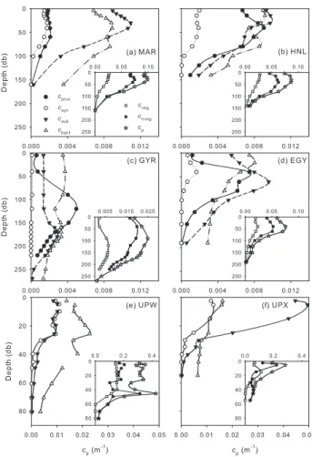
phyto-Fig. 6. Mean group-specific particle beam attenuation coeffi-cients for Prochlorococcus (cproc), Synechococcus (csyn),
picophy-toeukaryotes (ceuk), bacterioplankton (cbact). Insets contain the
vegetal (cveg), non-vegetal (cnveg), and total particle beam
atten-uation coefficient (cp) in m−1. For MAR (a), HNL (b), GYR (c),
EGY (d), UPW (e) and UPX (f). Note that UPW and UPX scales are equal to each other and different from the rest. For MAR, HNL, GYR and EGY all scale are the same except for GYR’s cp, cvegand
cnveg.
plankton biomass (Table 1). Except for Synechococcus and picophytoeukaryotes, no statistically significant correlations were observed between picoplanktonic groups (Table 1).
3.2 Picoplankton contributions to cp, a proxy for POC
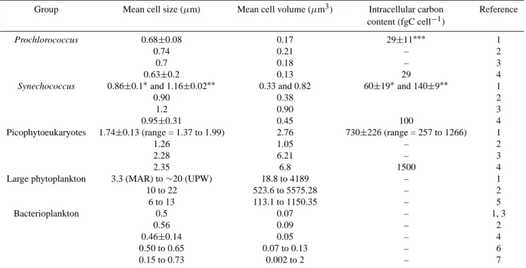
Mean pico- and large phytoplankton cell sizes used to esti-mate the group-specific attenuation cross sections are sum-marized in Table 2 and compared with values from the literature. These values and the standard errors associ-ated with them (Table 2) were obtained using the relation-ship established between mean FSC and cell size (Fig. 3a). The largest size difference between previous studies and the present one was observed for the picophytoeukary-otes (Table 2). For this group, the attenuation coefficients
Table 2. Picoplankton mean cell size (µm), volume (µm3) and intracellular carbon content (fgC cell−1).
Group Mean cell size (µm) Mean cell volume (µm3) Intracellular carbon Reference content (fgC cell−1)
Prochlorococcus 0.68±0.08 0.17 29±11∗∗∗ 1
0.74 0.21 – 2
0.7 0.18 – 3
0.63±0.2 0.13 29 4
Synechococcus 0.86±0.1∗and 1.16±0.02∗∗ 0.33 and 0.82 60±19∗and 140±9∗∗ 1
0.90 0.38 2
1.2 0.90 3
0.95±0.31 0.45 100 4
Picophytoeukaryotes 1.74±0.13 (range = 1.37 to 1.99) 2.76 730±226 (range = 257 to 1266) 1
1.26 1.05 – 2
2.28 6.21 – 3
2.35 6.8 1500 4
Large phytoplankton 3.3 (MAR) to ∼20 (UPW) 18.8 to 4189 – 1
10 to 22 523.6 to 5575.28 – 2 6 to 13 113.1 to 1150.35 – 5 Bacterioplankton 0.5 0.07 – 1, 3 0.56 0.09 – 2 0.46±0.14 0.05 – 4 0.50 to 0.65 0.07 to 0.13 – 6 0.15 to 0.73 0.002 to 2 – 7 1This study
2Chung et al. (1998); Equatorial Pacific 3Claustre et al. (1999); Tropical Pacific Ocean
4Zubkov et al. (2000); North and South Atlantic Subtropical Gyres 5Oubelkheir et al. (2005); Mediterranean Sea
6Ulloa et al. (1992); Western North Atlantic
7Gundersen et al. (2002); Bermuda Atlantic Time Series (BATS)
∗For most of the transect and∗∗for UPX, the most coastal station
∗∗∗Obtained using the conversion factor 171±15 fg C µm3derived from Synechococcus (see Sect. 2.1)
were determined by changes in both size (decreasing to-wards the coast; see Supp. Mat.: www.biogeosciences. net/4/837/2007/bg-4-837-2007-supplement.pdf) and abun-dance, when considering a constant refractive index. As a result, for instance, an average decrease in mean cells size of 0.22 µm (0.0056 µm3) from MAR to HNL
(see Supp. Mat.: www.biogeosciences.net/4/837/2007/ bg-4-837-2007-supplement.pdf) counteracts the higher cell abundance in the latter (Fig. 6g; Table 2) to modulate ceuk
along the transect (Figs. 6 and 7). In the case of Prochloro-coccus, the mean value presented in Table 2 was obtained from samples taken at different depths along the entire tran-sect, except at the centre of the gyre where the FSC signal could only be retrieved at depth. Larger cell sizes for this group were always found in deeper samples (not shown).
Along the transect, the shape and magnitude of the ver-tical cpprofiles were mainly determined by the non-vegetal
compartment, with cpand cnvegpresenting the same vertical
pattern at all long stations (Fig. 6). At MAR and HNL, cp
was rather homogeneous in the top 50 m and declined
be-low this depth, whereas cnvegdecreased systematically with
depth (Figs. 6a and b). At GYR cp and cnveg subsurface
maxima were both observed around 100 m, these two vari-ables being highest around 40 m at EGY (Figs. 6c and d). Both cp and cvegtended to be lower under hyper- and
olig-otrophic conditions at the centre of the gyre and were highest at UPW (Fig. 6). Both Prochlorococcus (when present) and picophytoeukaryotes usually presented subsurface maxima in their attenuation coefficients (e.g. at GYR around 125 m for the former and between 150 and 250 m for the latter; Fig. 6c) except at UPW, where ceuk tended to decrease
be-low 30 m (Fig. 6e). UPX profiles were included to highlight the differences observed with UPW, the other upwelling sta-tion (Figs. 6e and f). No large phytoplankton peaks (>3 µm) were detected between Station 3 and 15, including GYR.
Total and group-specific integrated attenuation coeffi-cients (0 to 1.5 Ze) tended all to decrease from the west-ern side towards the center of the gyre and increased again towards the coast (Fig. 7a). The integrated non-vegetal attenuation coefficient (detritus + bacterioplankton
Fig. 7. Integrated attenuation coefficients for Prochlorococcus (Proc), Proc + Synechococcus (Cyano), Cyano + picophytoeukary-otes (Picophyto), Picophyto + nanophytoplankton (Phyto), Phyto + bacterioplankton (Phyto + Bact), Phyto + Bact + heterotrophic pro-tists (Phyto + Bact + Hetero) and Phyto + Bact + Hetero + detritus
(cp) in the 0 to 1.5 Ze layer (a) and the 0 to 50 m layer (c). The
con-tributions by Prochlorococcus (cproc), picophytoeukaryotes (ceuk),
detritus (cdet), vegetal (cveg) and non-vegetal (cnveg) particles to the
corresponding total integrated attenuation coefficients are shown in
(b) and (d). The top black lines in (a) and (c) correspond to the
total integrated particle beam attenuation coefficient (cp, left hand
axis) and particulate organic carbon concentration (POC, right hand axis) estimated from cpusing Claustre et al. (1999) relationship (see
Sect. 2.2; Eq. 5). M, O and E stand for meso-, oligo- and eutrophic conditions (top of each panel). H, G, EG and W indicate HNL, GYR, EGY and UPW stations.
+ heterotrophic organisms) was quite variable, constituting
≥70% of c0−1.5 Zein most of the transect, reaching the
high-est (83%) and lowhigh-est (50%) contributions at GYR and UPW, respectively (Fig. 7b). Detritus being estimated by difference (Eq. 4), cdet and cveg’s contributions to c0−1.5 Ze followed
a general opposite trend, presenting similar values near the meso-oligotrophic limits (∼128 and 87◦W) (Fig. 7b). De-tritus contribution to c0−1.5 Ze was always ≤50%, the
low-est values being associated with highlow-est vegetal contribu-tions (Fig. 7b). Interestingly, between the two extreme trophic conditions encountered at GYR (hyper-oligotrophic; see Claustre et al., 2007) and UPW (eutrophic), c0−1.5 Ze
and integrated cveg increased ∼2- and 6-fold, respectively,
whereas integrated cnveg and cdet were only ∼1.2- and
1.1-fold higher at the upwelling station (Fig. 7a). Furthermore, in terms of contribution to c0−1.5 Ze, cveg was ∼3 times higher
at UPW, cnveg and cdet representing only about half of the
percentage estimated at GYR (Fig. 7b).
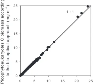
Fig. 8. Picophytoeukaryotes carbon biomass estimated from
intra-cellular carbon content (see Sect. 2.1) compared to that estimated by calculating ceukcontribution to cp, the latter assumed to be
equiv-alent to POC (see Sect. 2.2). Note that both approaches gave very similar results. 1:1 indicates the 1-to-1 line relating both estimates.
Mean integrated Prochlorococcus (when present) and pi-cophytoeukaryotes contributions to c0−1.5 Ze for the whole
transect were equivalent (9.7±4.1 and 9.4±3.8%, respec-tively), although the latter were clearly more important un-der mesotrophic conditions in both absolute values (Fig. 7a) and relative terms (Fig. 7b). Synechococcus attenuation co-efficients were too low (Fig. 7a) to contribute significantly to cp (only 1.0±1.0% on average), so we did not include
them in Fig. 7b. Bacterioplankton attenuation coefficients varied little along the transect and were always lower than all phytoplankton combined (Fig. 7b). Large phytoplankton at-tenuation coefficients were lower than that of the picophyto-plankton (cyanobacteria and picophytoeukaryotes combined) in the western part of the transect and higher or similar near the coast (Fig. 7a), their contributions to cp following the
same trend (included in cveg’s contribution, Fig. 7b).
When comparing c0−1.5 Ze to c0−50 mand their integrated
group-specific attenuation coefficients, it becomes clear that not considering data below 50 m leads to very different re-sults in most of the transect and especially at the centre of the gyre (Figs. 7a and c). For instance, whereas at UPW
c0−1.5 Ze and c0−50 m were equivalent, the former is 2- and
the latter 13-fold higher than the corresponding GYR inte-grated values (Figs. 7a and c). Similarly, there was a 2-fold difference in cveg’s contributions to c0−1.5 Zeand c0−50 m at
Fig. 9. Picophytoeukaryotes contribution to the photosynthetic
car-bon biomass as derived from ceuk’s contribution to cvegby
apply-ing Eq. (5) (bio-optical method) and as obtained usapply-ing intracellu-lar carbon contents in Table 2 to estimate picophytoplankton car-bon biomass (a). When comparing the results obtained using both approaches, it can clearly be seen that the contributions estimated using the intracellular carbon (C) content approach are lower than those estimated using the bio-optical approach, with almost all data points being below the 1-to-1 line relating both estimates (b).
3.3 Phytoplanktonic carbon biomass stocks and spatial variability
To avoid the use of carbon conversion factors from the litera-ture, in the present work we used two different approaches to estimate the picophyoteukaryotes carbon biomass: (1) from intracellular carbon content (Fig. 3b; see Sect. 2.1) and (2) calculating ceuk contribution to cp, the latter assumed to be
equivalent to POC (see Sect. 2.2). Both approaches gave very similar results (Fig. 8), indicating that the premise that all pi-cophytoeukaryotic organisms have the same refractive index (∼1.05) is valid for the sampled transect, even if we know that this group is usually constituted by diverse taxa (Moon-van der Staay et al., 2001). The above provides strong sup-port for the use of optical techniques and theory to determine picophytoeukaryotes carbon biomass, under the sole condi-tion of using actual mean cell sizes.
The deconvolution of cpindicates that at the centre of the
gyre (∼120.36 to 98.39◦W or Station 7 to 14+GYR) the photosynthetic biomass, which was dominated by picophyto-plankton, constituted ∼18% of the total integrated cpor POC
(Fig. 7b). Even more interestingly, when looking at the vege-tal compartment alone, ∼43% of this photosynthetic biomass would correspond to the picophytoeukaryotes (Fig. 9a; filled circles). Let us now assume that the contribution to in-tegrated cp by all phytoplanktonic groups is representative
of their contribution to POC, as proven for the toeukaryotes (see above). Under this assumption, picophy-toeukaryotes would constitute 51% of the total phytoplank-ton carbon biomass (large phytoplankphytoplank-ton included) at MAR, about 39% at HNL and GYR and 43% at EGY (Fig. 9a; filled circles). At UPW, however, where mean integrated POC es-timated from cp(see Sect. 2.2) was ∼6 g m−2(right axis on
Fig. 7a), picophytoeukaryotes would only constitute 5% of the photosynthetic biomass (Fig. 9a; filled circles). When considering the whole transect, picophytoeukaryotes mean contribution to the total photosynthetic carbon biomass (i.e.
ceuk’s mean contribution to cp) was ∼38%.
Intracellular carbon contents used to estimate picophyto-plankton biomass through the relationship established with FSC (Fig. 3b) are given in Table 2. Contributions to POC by Prochlorococcus and Synechococcus were ∼1.7 and 1.5 times higher when estimated using this approach rather than attenuation coefficients (not shown). Using these higher val-ues for cyanobacteria and assuming that the contribution by large phytoplankton is equivalent to clarge’s contribution
to cp, picophytoeukaryotes mean contribution to the total
photosynthetic carbon biomass along the transect would be
∼30%, representing ∼28 instead of 43% at the centre of the gyre (Fig. 9a; empty circles). These contributions are slightly lower than the ones estimated through the optically-based ap-proach, with almost all data points being below the 1-to-1 line relating both estimates (Fig. 9b).
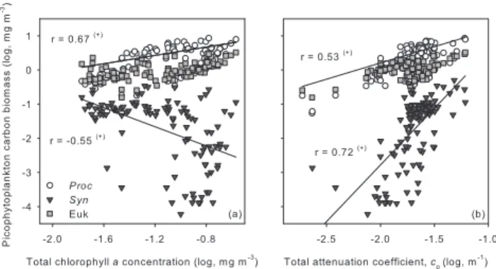
Regarding spatial variability, both Tchla (r=0.67,
p<0.001) and cp (r=0.53, p<0.001) were correlated to
the dominant picophytoplankton carbon biomass, i.e. Prochlorococcus + picophytoeukaryotes, between Stations 3 and 15, GYR included (Fig. 10). The results of a t-test on the z-transformed correlation coefficients (Zokal and Rohlf, 1994) indicates that both correlations are not sig-nificantly different (p>0.05). Therefore, Tchla and cp
were equally well correlated to the picophytoplanktonic biomass. Synechococcus biomass, on the other hand, was negatively correlated to Tchla (Fig. 10a) and positively to
cp (Fig. 10b). However, despite the differences observed
between this cyanobacterium and the other two groups, cor-relation coefficients calculated for total picophytoplankton biomass (i.e. dominant + Synechococcus; not shown) were not significantly different (p>0.05) from those calculated for the dominant groups (Fig. 10). Synechococcus had no influence on the general relationships because of its negligible biomass. Tchla and cp were therefore useful in
tracing total picophytoplanktonic carbon biomass in the part of the transect where no large phytoplankton was detected (i.e. Stations 3 to 15+GYR).
4 Discussion and conclusion 4.1 Picoplankton abundance
Macroecological studies indicate that 66% of the variance in picophytoplankton abundance can be explained by tempera-ture (the dominant factor), nitrate and chlorophyll a concen-tration (Li, 2007). It has also been established that higher Prochlorococcus abundances are observed in more stratified waters, whereas Synechococcus and picophytoeukaryotes are more abundant when mixing prevails (e.g. Blanchot and
Rodier, 1996; Shalapyonok et al., 2001). Across the eastern South Pacific Ocean temperature, especially for Prochloro-coccus and bacterioplankton (Fig. 5), and nitrate concentra-tion along the transect (see Fig. 4b) appear important in mod-ulating picophytoplankton abundance, their influence vary-ing accordvary-ing to the prevailvary-ing trophic conditions.
As expected (e.g. Gasol and Duarte, 2000), integrated bacterioplankton abundances covaried with phytoplankton biomass (Table 1). Integrated picophytoeukaryotes abun-dance was the only one to vary independently from Tchla when considering the whole transect (Table 1), suggesting that the factors controlling picophytoplankton population, such as sinking, sensitivity to radiation, grazing, viral in-fection, etc. (Raven, 2005) acted differently on this group. Thus, the ecology of picophytoeukaryotes needs to be stud-ied in further detail. Across the eastern South Pacific, surface bacterioplankton concentrations were similar to those found by Grob et al. (2007) at 32.5◦S. However, in the deep layer of the hyper-oligotrophic part of the gyre (200 m) this group was 2.5 times more abundant than published by Grob et al. (2007). Given the correlation between integrated bacteri-oplankton abundance and Tchla concentration (Table 1), the latter could be attributed to the presence of deep Prochloro-coccus and picophytoeukaryotes maxima that were not ob-served by Grob et al. (2007). Such deep maxima are a recur-rent feature in the oligotrophic open ocean (Figs. 4e and g; Table 3). Along the transect, picophytoplankton abundances were usually within the ranges established in the literature for oligo-, meso- and eutrophic regions of the world’s ocean (see Table 3). It is worth noticing that our estimates for sur-face Prochlorococcus abundance were, to our knowledge, the lowest ever estimated for the open ocean (see Table 3), al-though a possible underestimation cannot be ruled out.
The presence of the mentioned groups under extreme poor conditions suggests a high level of adaptation to an environ-ment where inorganic nutrients are below detection limit. Al-though little is known on picophytoeukaryotes metabolism, several cyanobacteria ecotypes have been shown to grow on urea and ammonium (Moore et al., 2002). Ammonium up-take at the centre of the gyre was low but still detectable (Raimbault et al., 2007). Considering that heterotrophic bac-teria would be responsible for ∼40% of this uptake in ma-rine environments (Kirchman, 2000), the possibility of sur-face picophytoplankton growing on this form of nitrogen at the centre of the gyre cannot be discarded.
4.2 Picoplankton contribution to cp
The larger increase of integrated cveg as compared to cnveg
observed between extreme trophic conditions (see Sect. 3.2) indicates that across the eastern South Pacific spatial variabil-ity in the vegetal compartment was more important than the non-vegetal one in shaping the water column optical prop-erties, at least the particle beam attenuation coefficient. As expected (e.g. Chung et al., 1996; Loisel and Morel, 1998;
Fig. 10. Log-log relationships for Prochlorococcus (Proc),
Syne-chococcus (Syn) and picophytoeukarytos (Euk) carbon biomass
(mg m−3) with total chlorophyll a concentration in mg m−3(a) and
total particle beam attenuation coefficient in m−1(b). Only data
from Stations 3 to 15 and GYR, where no large phytoplankton cells were detected, and between the surface and 1.5 Ze are included (see Sect. 2.2). Correlation coefficients (r) were calculated for the sum of Proc and Euk (upper values) and for Syn carbon biomass (lower values) with Tchla (a) and cp(b).(+)indicates p<0.001.
Claustre et al., 1999), cp and cveg tended to be lower
un-der hyper- and oligotrophic conditions at the centre of the gyre and were highest at UPW. Here, the highest cpand cveg
were associated with mature upwelling conditions character-ized by the highest primary production (Moutin et al., 2007) and Tchla (Fig. 4d), and low nutrient concentration (Fig. 4b; Raimbault et al., 2007).
Although the non-vegetal particles tended to dominate the
cp signal, and therefore POC, regardless of trophic
condi-tion (Fig. 7b; e.g. Chung et al., 1998; Claustre et al., 1999; Oubelkheir et al., 2005), this dominance seems to weaken from oligo- to eutrophic conditions (Claustre et al., 1999; this study). Here we showed that under mature upwelling condi-tions (UPW) the contribution by vegetal and non-vegetal par-ticles may even be equivalent (Fig. 7b), in contrast with the invariant ∼80% cnvegcontribution estimated by Oubelkheir
et al. (2005) for different trophic conditions. We therefore emphasize the importance of using complementary data to interpret bio-optical measurements since, for instance, the
∼2.3-fold difference in cveg’s contribution to cpobserved
be-tween our UPW results and those published by Ouberkheir et al. (2005) seems to be related to the state of development of the upwelling event (mature versus early).
At the hyper-oligotrophic centre of the gyre, ceuk
con-tribution to c0−1.5 Ze was equivalent to the one possibly
overestimated (because of the larger cell size assumed) by Claustre et al. (1999). The above highlights the importance of making good size estimates when decomposing the to-tal attenuation signal since, for example, a difference of 1.02 µm in size leads to a 10-fold difference in the scatter-ing cross-section calculated for picophytoeukaryotes (Claus-tre et al., 1999; Oubelkheir et al., 2005). In the present
Table 3. Prochlorococcus, Synechococcus and picophytoeukaryotes abundances (×103cells ml−1) registered during spring time in different
regions of the world’s ocean under varying trophic conditons.
Trophic condition Prochlorococcus Synechococcus Picophytoeukaryotes Reference Hyper-oligotrophic 16–18∗ 150–160 (125 m) 1.2–1.6∗ 0.8–1.4 (125 m) 0.76–1.3∗ 1.8–2.3 (175 m) 1 (GYR) Oligotrophic 35–40∗ 200–250 (50–75 m) 6.9–8.6∗ 20 (50 m) 4.5–4.9∗ 14 (60 m) 1 (EGY) 240 (0 to 100 m) 1.5 (0 to 100 m) 0.8-1 (0 to 100 m) 2 30∗ 200 (120 m) 0.7∗ 1–1.5 (50–125 m) 0.5∗ 2 (140–150 m) 3 100–150∗ 100 (120 m) 3–30∗ 1 (120–160 m) 0.6–2∗ 1–2 (80–120 m) 4 115∗ 150–200 (50–100 m) 0.2–1 (0 to 100 m) 0.25–0.5∗ Up to 3 (100 m) 5 60 (0 to 100 m) 2.5 (0 to 50–100 m) 2–4∗ 2 (100 m) 6 HNL 200 (surf) 270 (30–60 m) 10–28 (surf) 25 (50 m) 5–9 (0 to 80 m) 1 150–300 (0 to 80 m) 3–5 (0 to 80 m) 0.6–1 (0 to 100 m) 3 200 (0 to 50 m) 100 (80 m) 8 (0 to 100 m) 3 (0 to 100 m) 7 200 (30 and 60 m) 15 and 13 (30 and 60 m) 6 and 5 (30 and 60 m) 8 Mesotrophic 50–60 (0 to 80 m) 17–20 (0 to 60 m) 3–5 (0 to 80 m) 1 (MAR) 30–200∗ 1–40 (100 m) 5–44∗ 0.2–3 (100 m) 3–18∗ 0.4–4 (100 m) 6 Eutrophic – 60–200 5–10 1 (UPW) – 50–250 10–60 9 – Up to 150 Up to 80–90 10 ∗ Surface data 1This study
2Campbell and Vaulot (1993); Subtropical North Pacific (ALOHA)
3Vaulot et al. (1999); Subtropical Pacific (16◦S; 150◦W). These authors considered their surface Prochlorococcus abundances as “severely
underestimated”.
4Zubkov et al. (2000); North and South Atlantic Subtropical Gyres 5Veldhuis and Kraay (2004); Eastern North Atlantic Subtropical Gyre 6Grob et al. (2007); Eastern South Pacific
7Mackey et al. (2002); Equatorial Pacific 8Landry et al. (2003); Equatorial Pacific
9Worden et al. (2004); Southern California Bight, North Pacific 10Sherr et al. (2005); Oregon upwelling ecosystem, North Pacific
work, picophytoplankton populations were isolated on board by flow-cytometry cell sorting in order to measure their ac-tual sizes using a particle counter (see Sect. 2.1). It is the first time to our knowledge that such direct measurements have been made in the field. For future studies we recom-mend to measure the different picophytoplankton mean cell sizes in situ for at least a few samples, including surface and deep populations in order to consider possible vertical vari-ability. If these samples are taken under different oceano-graphic conditions, we also recommend including samples from each one of these conditions.
By establishing a relationship with FSC to estimate ac-tual picophytoplankton cell size (Fig. 3a), we confirmed that picophytoeukaryotes were more important contribu-tors to cp than cyanobacteria under both meso- and
eu-trophic conditions (Claustre et al., 1999). The uncer-tainties in this relationship are larger for cyanobacteria (lower part of the curve; Fig. 3a) than for picophytoeukary-otes. However, Prochlorococcus and Synechococcus’ mean cell sizes measured in situ were ≤0.59 (only one isolated population could be measured with the Coulter Counter, the rest being too small) and ≤0.87 µm, respectively (see
Table A, Supp. Mat.: www.biogeosciences.net/4/837/2007/ bg-4-837-2007-supplement.pdf). We therefore believe that these group’s mean cell sizes, and therefore their contribu-tions to cpalong the transect, may have been at most
over-rather than underestimated by this relationship. Differences in cell size (Table 2) would also explain the much lower Synechococcus contribution to cp observed in the
hyper-oligotrophic centre of the gyre compared to that published by Claustre et al. (1999) for the tropical Pacific (16◦S, 150◦W). Only data collected at local noon time were used to es-timate group-specific attenuation coefficients, to avoid er-rors associated with the natural diel variability that has been observed in the refractive index of picophytoplankton cells from culture (e.g. Stramski et al., 1995; DuRand and Ol-son, 1998; DuRand et al., 2002). Here we showed that the premise that all picophytoeukaryotes are homogeneous spheres with the same refractive index of 1.05 (assumptions of the anomalous diffraction approximation) is valid for the sampled transect when actual mean cell sizes are used. In the case of Synechococcus, a high refractive index of 1.083 (Aas, 1996) would only increase this group’s mean attenua-tion cross-secattenua-tion by an almost negligible 6%. Given their low abundance compared to the other groups, the resulting increase in their contribution to cpwould be even lower.
If Prochlorococcus were to have a refractive index of 1.06 for instance, their mean attenuation cross-section would be 43% higher than the one calculated here. Nevertheless, the resulting Prochlorococcus’ contribution to cp for the entire
transect would only be 4±2% higher. However, this group’s contribution to cveg would increase by 18±2% on average,
constituting up to 99% of the vegetal compartment under hyper-oligotrophic conditions. Such high contribution con-tradicts both HPLC (dv-chla to Tchla ratios of ∼0.2 to 0.5; see Ras et al., 2007) and flow cytometry data (see Syne-chococcus and picophytoeukaryotes abundances; Figs. 4f and g) and appears hence not possible. We therefore be-lieve that the assumption of a refractive index of 1.05 for cyanobacteria is appropriate for the purposes of the present work. It is worth noticing that lower refractive indexes for these two groups would only reduce their contribution to cp
(and therefore POC) and cveg, the contribution by
picophy-toeukaryotes resulting even more important than stated in this work.
Regarding mean cell size, deep Prochlorococcus cells are larger than surface ones (e.g. Li et al., 1993; this study). The former are better represented than the latter in the data set used to estimate mean Prochlorococcus cell size for the tran-sect, since surface FSC signals could not be retrieved for a large area at the centre of the gyre. We therefore consider that the mean cell size used here for this group could be at most overestimated, i.e. biased towards a larger value due to the fewer surface data available. Hence, picophytoeukary-otes’ contributions to cvegcould only be underestimated. The
above highlights the importance of this group in terms of photosynthetic biomass in the open ocean.
Definitively the largest uncertainties in the deconvolution of cp are related to the determination cbact and chet, which
have a direct influence on cdet’s estimates (see Sect. 2.2,
Eq. 4). First, bacterioplankton cells were assumed to have a mean cell size of 0.5 µm. Taking the minimum and max-imum sizes presented in Table 2 (i.e. 0.46 and 0.73 µm), the scattering cross section for bacterioplankton would be
∼28% lower and 4.5 times higher than the one used here, re-spectively. The lower scattering cross sections for these two groups would imply an underestimation of detritus’ contribu-tion to cpof only 11±3% on average for the entire transect.
A scattering cross section 4.5 times higher (i.e. 0.73 µm of mean cell size) would imply contributions ≥100% to cp, and
therefore POC, by bacteria and heterotrophic protests alone, which seems unrealistic. Using a mean cell size of 0.6 µm, i.e. the average value between 0.46 and 0.73 µm, leads to the same kind of overestimation of the heterotrophic contribu-tions to cp. Based on the above, we consider the assumption
of a 0.5 µm mean cell size for bacterioplankton to be ap-propriate for our estimates, since at most it would slightly underestimate detritus.
Following Claustre et al. (1999), here we assumed that
chet=2 cbact (see Sect. 2.2, Eq. 3). The range reported by
Morel and Ahn (1993) for this conversion factor is 1.8 to 2.4. Using these values instead of 2 would result in an average increase and decrease in cdet’s contribution to cp
across the eastern South Pacific of 2±1% and 4±2%, respec-tively, which in both cases is negligible. It is worth noticing that even if larger errors were associated with the assump-tions made in this work regarding bacterioplankton and het-erotrophic protists, our results and conclusions regarding pi-cophytoeukaryotes contributions to cp, and therefore POC,
and to the photosynthetic carbon biomass across the eastern South Pacific would not change.
4.3 Phytoplankton carbon biomass stocks and spatial vari-ability
One of the most important observations of the present study is that spatial variability in the open-ocean, where no large phytoplankton was detected, picophytoplankton car-bon biomass can be traced by changes in both Tchla and cp
(Fig. 10). While chlorophyll concentration has widely been used as a proxy for photosynthetic carbon biomass, the use of cpis more controversial. For instance, although cpseems
to be a better estimate of phytoplankton biomass than Tchla in Case I waters (Behrenfeld and Boss, 2003) and within the mixed layer of the eastern Equatorial Pacific (Behrenfeld and Boss, 2006), chlorophyll concentration would work better in subtropical stratified waters (Huot et al., 2007). Our re-sults indicate that Tchla and cpwould be equally useful
esti-mates of photosynthetic carbon biomass in the South Pacific gyre, where it is mainly constituted by picophytoplankton (≤3 µm). However, it is important to highlight that in order to estimate the photosynthetic carbon biomass from cpit is
necessary to have information or make some assumptions on the contributions by vegetal and non-vegetal particles to this coefficient. In this case, picophytoplankton biomass and cp
were positively correlated such as that the former could be retrieved from the latter. Despite of the stated limitations, the bio-optical approach used in the present work could be a good alternative for large scale open ocean surveys, espe-cially considering that cpmeasurements are much less
time-consuming than determining chlorophyll concentration and can also be obtained at a much higher vertical resolution. Further research should be done to test the ability of cp in
tracing phytoplankton biomass in the ocean.
Although when present Prochlorococcus largely domi-nates in terms of abundance, the picophytoeukaryotes would constitute ∼38% on average of the total integrated phyto-plankton carbon biomass (Prochlorococcus + Synechococ-cus + picophytoeukaryotes + large phytoplankton) estimated from ceuk’s contribution to cveg (Fig. 9a, filled circles;
see Sect. 3.3). Furthermore, under oligotrophic conditions this group constituted ∼43% of the photosynthetic carbon biomass. Previous studies indicate that picophytoeukaryotes largely dominate the vegetal compartment in the equatorial Pacific (DuRand et al., 1996; Claustre et al., 1999) and the pi-cophytoplanktonic carbon biomass across the eastern South Pacific along 32.5◦S (Grob et al., 2007). Here we showed that this group constitutes a very important and in some cases a dominant fraction of cvegacross the eastern South Pacific,
confirming the findings by Grob et al. (2007). The above also agrees with what has been observed in the North and South Atlantic Subtropical Gyres (Zubkov et al., 2000). Pi-cophytoeukaryotes also dominated the picophytoplanktonic carbon biomass in the coastal region, as previously indicated by Worden et al. (2004) and Grob et al. (2007).
Picophytoeukaryotes contributions obtained by estimat-ing cyanobacteria biomass from intracellular carbon content were probably underestimated compared to those obtained using the bio-optical approach (Fig. 9b) because of the con-version factor used for Prochlorococcus (Table 2). We be-lieve that establishing a relationship between intracellular carbon content and FSC for this cyanobacterium, as we did for Synechococcus and picophytoeukaryotes, would lead to contributions similar to those estimated using attenuation co-efficients. It is worth noticing that higher or lower cyanobac-teria carbon biomasses would only modify the y-intercept of the biomass relationships with Tchla and cp(Fig. 10), but not
their slope or their strength.
When normalized to 1 µm3, maximal growth rates estimated for picophytoeukaryotes are higher than for Prochlorococcus (Raven, 2005, and references therein). Considering that the former are ∼16 times larger than the latter in terms of mean cell volume, the amount of car-bon passing through the picophytoeukaryotes could be very important. For the same reason, this group could also be the most important contributor to export fluxes in the open ocean, since picophytoplankton share of this carbon pathway
seems to be much more important than previously thought (Richardson and Jackson, 2007; Barber, 2007). The role of this group in carbon and energy flow would therefore be cru-cial.
Picophytoeukaryotes carbon biomass in the open ocean seems to be much more important than previously thought. Across the eastern South Pacific, this group’s biomass is almost equivalent to that of Prochlorococcus under hyper-oligotrophic conditions and even more important under mesotrophic ones. The role of picophytoeukaryotes in bio-geochemical cycles needs to be evaluated in the near future. Further attention needs to be focused on this group.
Acknowledgements. This work was supported by the Chilean
National Commission for Scientific and Technological Research (CONICYT) through the FONDAP Program and a graduate fel-lowship to C. Grob; the ECOS (Evaluation and Orientation of the Scientific Cooperation, France)-CONICYT Program, the French program PROOF (Processus Biogeochimiques dans l’Oc´ean et Flux), Centre National de la Recherche Scientifique (CNRS), the Institut des Sciences de l’Univers (INSU), the Centre National d’Etudes Spatiales (CNES), the European Space Agency (ESA), the National Aeronautics and Space Administration (NASA) and the Natural Sciences and Engineering Research Council of Canada (NSERC). This is a contribution of the BIOSOPE project of the LEFE-CYBER program. D. Tailliez and C. Bournot are warmly thanked for their efficient help in CTD rosette management and data processing. We also thank the scientific party and the Captain and crew of the RV L’Atalante during the BIOSOPE Expedition; F. Thi`eche for her help with laboratory work; L. Far´ıas and M. Gallegos for organic carbon analyses, B. Gentili for PAR data processing and R. Wiff for help with statistical analyses.
Edited by: E. Boss
References
Aas, E.: Refractive index of phytoplankton derived from its metabo-lite composition, J. Plankton Res., 18, 2223–2249, 1996. Antoine, D., Andr´e, J. M., and Morel, A.: Oceanic primary
produc-tion II. Estimaproduc-tion at global scale from satellite (Coastal Zone Color Scanner) chlorophyll, Global Biogeochem. Cycles, 10, 57–69, 1996.
Barber, R. T.: Picoplankton Do Some Heavy Lifting, Science, 315, 777–778, 2007.
Behrenfeld, M. J. and Boss, E.: The beam attenuation to chlorophyll ratio: an optical index of phytoplankton physiology in the surface ocean?, Deep Sea Res. Part I, 50, 1537–1549, 2003.
Behrenfeld, M. J. and Boss, E.: Beam attenuation and chloro-phyll concentration as alternative optical indices of phytoplank-ton biomass, J. Mar. Res., 64, 431–451, 2006.
Bissett, W. P., Walsh, J. J., Dieterle, D. A., and Carder, K. L.: Car-bon cycling in the upper waters of the Sargasso Sea: I. Numerical simulation of differential carbon and nitrogen fluxes, Deep Sea Res. I, 46, 205–269, 1999.
Blanchot, J. and Rodier, M.: Picophytoplankton abundance and biomass in the western Tropical Pacific Ocean during the 1992
El Nino year: Results from flow cytometry, Deep-Sea Res., 43, 877–896, 1996.
Campbell, L. and Vaulot, D.: Photosynthetic picoplankton commu-nity structure in the subtropical North Pacific Ocean near Hawaii (station ALOHA), Deep Sea Res. I, 40, 2043–2060, 1993. Carr, M.-E., Friedrichs, M. A. M., Schmeltz, M., Aita, M. N.,
Antoine, D., Arrigo, K. R., Asanuma, I., Aumont, O., Barber, R., Behrenfeld, M., Bidigare, R., Buitenhuis, E. T., Campbell, J., Ciotti, A., Dierssen, H., Dowell, M., Dunne, J., Esaias, W., Gentili, B., Gregg, W., Groom, S., Hoepffner, N., Ishizaka, J., Kameda, T., Qu´er´e, C. L., Lohrenz, S., Marra, J., M´elin, F., Moore, K., Morel, A., Reddy, T. E., Ryan, J., Scardi, M., Smyth, T., Turpie, K., Tilstone, G., Waters, K., and Yamanaka, Y.: A comparison of global estimates of marine primary production from ocean color, Deep Sea Res. II, 53, 741–770, 2006. Chavez, F. P., Buck, K. R., Bidigare, R. R., Karl, D. M., Hebel,
D., Latasa, M., and Campbell, L.: On the chlorophyll a reten-tion properties of glass-fiber GF/F filters, Limnol. Oceanogr., 40, 428–433, 1995.
Chen, C.-T. A., Liu, K.-K., and MacDonald, R. W.: Continental margin exchanges. Ocean Biogeochemistry, in: The Role of the Ocean Carbon Cycle in Global Change, edited by: Fasham, M. J. R., IGBP Book Series, Springer, 53–97, 2003.
Chisholm, S. W., Olson, R. J., Zettler, E. R., Goericke, R., Wa-terbury, J. B., and Welschmeyer, N. A.: A novel free-living prochlorophyte occurs at high cell concentrations in the oceanic euphotic zone, Nature, 334, 340–343, 1988.
Chung, S. P., Gardner, W. D., Richardson, M. J., Walsh, I. D., and Landry, M. R.: Beam attenuation and microorganisms: spatial and temporal variations in small particles along 14O′′W during the 1992 JGOFS EqPac transects, Deep Sea Res. II, 43, 1205– 1226, 1996.
Chung, S. P., Gardner, W. D., Landry, M. R., Richardson, M. J., and Walsh, I. D.: Beam attenuation by microorganisms and detrital particles in the Equatorial Pacific, J. Geophys. Res., 103(C6), 12 669–12 681, 1998.
Claustre, H., Morel, A., Babin, M., Cailliau, C., Marie, D., Marty, J. C., Tailliez, D., and Vaulot, D.: Variability in particle at-tenuation and chlorophyll fluorescence in the Tropical Pacific: Scales, patterns, and biogeochemical implications, J. Geophys. Res., 104(C2), 3401–3422, 1999.
Claustre, H., Huot, Y., Obernosterer, I., Gentili, B., Tailliez, D., and Lewis, M.: Gross community production and metabolic bal-ance in the South Pacific Gyre, using a non intrusive bio-optical method, Biogeosciences Discuss., 4, 3089–3121, 2007, http://www.biogeosciences-discuss.net/4/3089/2007/.
DuRand, M. D. and Olson, R. J.: Contributions of phytoplankton light scattering and cell concentration changes to diel variations in beam attenuation in the equatorial Pacific from flow cytomet-ric measurements of pico-, ultra- and nanoplankton, Deep Sea Res. Part II, 43, 891–906, 1996.
DuRand, M. D. and Olson, R. J.: Diel patterns in optical properties of the chlorophyte Nannochloris sp.: Relating individual-cell to bulk measurements, Limnol. Oceanogr., 43, 1107–1118, 1998. DuRand, M. D., Green, R. E., Sosik, H. M., and Olson, R. J.: Diel
variations in optical properties of Micromonas pusilla (Prasino-phyceae), J. Phycol., 38, 1132–1142, 2002.
Falkowski, P. G., Barber, R. T., and Smetacek, V.: Biogeochemical Controls and Feedbacks on Ocean Primary Production, Science,
200–206, 1998.
Field, C. B., Behrenfeld, M. J., Randerson, J. T., and Falkowski, P.: Primary Production of the Biosphere: Integrating Terrestrial and Oceanic Components, Science, 281, 237–240, 1998.
Gardner, W. D., Mishonov, A. V., and Richardson, M. J.: Global POC concentrations from in-situ and satellite data, Deep Sea Res. II, 53, 718–740, 2006.
Gasol, J. M. and Duarte, C. M.: Comparative analyses in aquatic microbial ecology: how far do they go?, FEMS Microbiol. Ecol., 31, 99–106, 2000.
Grob, C., Ulloa, O., Li, W. K. W., Alarc´on, G., Fukasawa, M., and Watanabe, S.: Picoplankton abundance and biomass across the eastern South Pacific Ocean along latitude 32.5◦S, Mar. Ecol. Prog. Ser., 332, 53–62, 2007.
Gundersen, K., Heldal, M., Norland, S., Purdie, D. A., and Knap, A. H.: Elemental C, N, and P cell content of individual bacteria collected at the Bermuda Atlantic Time-series Study (BATS) site, Limnol. Oceanogr., 47, 1525–1530, 2002.
Huot, Y., Babin, M., Bruyant, F., Grob, C., Twardowski, M. S., and Claustre, H.: Does chlorophyll a provide the best index of phytoplankton biomass for primary productivity studies?, Bio-geosciences Discuss., 4, 707–745, 2007,
http://www.biogeosciences-discuss.net/4/707/2007/.
Kirchman, D. L.: Uptake and regeneration of inorganic nutrients by marine heterotrophic bacteria, in: Microbial ecology of the oceans, edited by: Kirchman, D. L., Wiley-Liss, NewYork, 261– 288, 2000.
Landry, M. R., Brown, S. L., Neveux, J., Dupouy, C., Blanchot, J., Christensen, S., and Bidigare, R. R.: Phytoplankton growth and microzooplankton grazing in high-nutrient, low-chlorophyll waters of the equatorial Pacific: Community and taxon-specific rate assessments from pigment and flow cytometric analyses, J. Geophys. Res., 108, 8142–8156, 2003.
Le Qu´er´e, C., Harrison, S. P., Prentice, I. C., Buitenhuis, E. T., Au-mont, O., Bopp, L., Claustre, H., Cunha, L. C. D., Geider, R., Giraud, X., Klaas, C., Kohfeld, K. E., Legendre, L., Manizza, M., Platt, T., Rivkin, R. B., Sathyendranath, S., Uitz, J., Wat-son, A. J., and Wolf-Gladrow, D.: Ecosystem dynamics based on plankton functional types for global ocean biogeochemistry models, Global Change Biol., 11, 2016–2040, 2005.
Li, W. K. W., Zohary, T., Yacobi, Y. Z., and Wood, A. M.: Ultraphy-toplankton in the eastern Mediterranean Sea: Towards deriving phytoplankton biomass from flow cytometric measurements of abundance fluorescence and light scatter, Mar. Ecol. Prog. Ser., 102, 79–87, 1993.
Li, W. K. W.: Primary production of prochlorophytes, cyanobacte-ria, and eucaryotic ultraphytoplankton: Measurements from flow cytometric sorting, Limnol. Oceanogr., 39, 169–175, 1994. Li, W. K. W.: Composition of ultraphytoplankton in the Central
North Atlantic, Mar. Ecol. Prog. Ser., 122, 1–8, 1995.
Li, W. K. W.: Plankton Populations and Communities, in: Marine Macroecology, edited by: Witman, J. and Kaustuv, R., University of Chicago Press, in press, 2007.
Loisel, H. and Morel, A.: Light scattering and chlorophyll concen-tration in case 1 waters: A reexamination, Limnol. Oceanogr., 43, 847–858, 1998.
Mackey, D. J., Blanchot, J., Higgins, H. W., and Neveux, J.: Phyto-plankton abundances and community structure in the equatorial Pacific, Deep Sea Res. II, 49, 2561–2582, 2002.