MIT Joint Program on the
Science and Policy of Global Change
Absolute vs. Intensity-Based Emission Caps
A. Denny Ellerman and Ian Sue WingReport No. 100
The MIT Joint Program on the Science and Policy of Global Change is an organization for research, independent policy analysis, and public education in global environmental change. It seeks to provide leadership in understanding scientific, economic, and ecological aspects of this difficult issue, and combining them into policy assessments that serve the needs of ongoing national and international discussions. To this end, the Program brings together an interdisciplinary group from two established research centers at MIT: the Center for Global Change Science (CGCS) and the Center for Energy and Environmental Policy Research (CEEPR). These two centers bridge many key areas of the needed intellectual work, and additional essential areas are covered by other MIT departments, by collaboration with the Ecosystems Center of the Marine Biology Laboratory (MBL) at Woods Hole, and by short- and long-term visitors to the Program. The Program involves sponsorship and active participation by industry, government, and non-profit organizations.
To inform processes of policy development and implementation, climate change research needs to focus on improving the prediction of those variables that are most relevant to economic, social, and environmental effects. In turn, the greenhouse gas and atmospheric aerosol assumptions underlying climate analysis need to be related to the economic, technological, and political forces that drive emissions, and to the results of international agreements and mitigation. Further, assessments of possible societal and ecosystem impacts, and analysis of mitigation strategies, need to be based on realistic evaluation of the uncertainties of climate science.
This report is one of a series intended to communicate research results and improve public understanding of climate issues, thereby contributing to informed debate about the climate issue, the uncertainties, and the economic and social implications of policy alternatives. Titles in the Report Series to date are listed on the inside back cover.
Henry D. Jacoby and Ronald G. Prinn,
Program Co-Directors
For more information, please contact the Joint Program Office
Postal Address: Joint Program on the Science and Policy of Global Change MIT E40-428
77 Massachusetts Avenue
Cambridge MA 02139-4307 (USA) Location: One Amherst Street, Cambridge
Building E40, Room 428
Massachusetts Institute of Technology Access: Phone: (617) 253-7492
Fax: (617) 253-9845
E-mail: g l o ba l ch a n g e @ m i t .e d u
Web site: h t t p:/ / m i t .e d u / g l o ba l ch a n g e /
Absolute vs. Intensity-Based Emission Caps
A. Denny Ellerman†
and Ian Sue Wing* Abstract
Cap-and-trade systems limit emissions to some pre-specified absolute quantity. Intensity-based limits, that restrict emissions to some pre-specified rate relative to input or output, are much more widely used in environmental regulation and have gained attention recently within the context of greenhouse gas (GHG) emissions trading. In this paper we provide a non-technical introduction to the differences between these two forms of emission limits. Our aim is not to advocate either form, but to elucidate the properties of each in a world where future emissions and GDP are not known with certainty. We argue that the two forms have identical effects in a world where future emissions and economic output (i.e., GDP) are known with certainty, and show that outcomes for marginal costs, abatement, emissions and welfare diverge only because of the variance of actual future GDP relative to its forecast expectation.
Contents
1. Introduction ... 1
2. Absolute vs. Intensity Limits: Similarities, Differences, and the Role of Uncertainty ... 2
3. A General Approach: Growth-Indexed Emission Limits ... 4
4. Criteria for Choosing the Degree of Indexation ... 6
5. Dynamic Properties... 8
6. Concluding Comments... 10
References ... 11
1. Introduction
Emissions can be limited by an absolute cap on the quantity of emissions or by some maximum allowable intensity relative to some measure of output or input, such as the number of cars or refrigerators purchased by consumers, the amount of energy input required by some production process, or even GDP. This intensity limit can be imposed either directly as an emission rate limit or an efficiency standard, or indirectly by means of technology mandates that have the same effect. Intensity limits are by far the more common method of limiting emissions in the field of environmental regulation, although absolute caps are now found in a number of programs.1 In the domain of greenhouse gas (GHG) emissions limitation, absolute limits have
† Joint Program on the Science & Policy of Global Change, Massachusetts Institute of Technology. Corresponding
author: MIT Bldg. E40-280, 1 Amherst St., Cambridge MA 02139. Phone: (617) 253-3551, [email protected].
* Center for Energy & Environmental Studies and Department of Geography & Environment, Boston University;
and Joint Program on the Science & Policy of Global Change, Massachusetts Institute of Technology
1 Prominent examples of absolute limits are the SO
2 trading (acid rain), RECLAIM, and Northeastern NOx Budget
programs in the U.S. and the proposed EU GHG emissions trading system. Familiar examples of intensity limits are the emission rate limits imposed on nearly all sources under State Implementation Plans in the U.S., best available control technology mandates, such as in the U.S. New Source Performance Standards or the EU Large Combustion Plant Directive, and the Corporate Average Fuel Economy standards in the U.S. and similar programs in Europe. Although many of the latter do not explicitly specify an emission rate, the effect of these programs is to reduce emission (or energy) intensity and to allow emissions to vary with the level of output. The UK Emissions Trading Scheme is unique in having two sectors, an absolute sector containing firms with absolute limits on GHG emissions and a relative sector containing firms with intensity limits, and allowing trading (with some restrictions) between the two sectors.
been adopted at the international level in the Kyoto Protocol, while President Bush, in rejecting the Kyoto Protocol, has established an intensity target for the U.S.2
This paper presents a brief, non-technical exploration of the properties of absolute and intensity-based limits on GHG emissions. Our goal is not to advocate either form of limit in the context of GHG emissions control, but simply to analyze the properties of each with respect to emissions and costs. In doing so we highlight an unavoidable trade-off between quantities and prices of abatement in choosing the form of the emissions limit. Our specific objectives are four-fold: to show (i) the definitional equivalence of absolute and intensity limits when GDP is certain, (ii) the differing effects of the two limits on emissions and cost when future GDP is uncertain, (iii) how these differing effects can be tuned to avoid undesirable variations in costs or emissions, and finally (iv) that any desired long-term trajectory of GHG emissions can be achieved by either an absolute or an intensity limit, or any combination thereof.
2. Absolute vs. Intensity Limits: Similarities, Differences, and the Role of Uncertainty A frequent misconception, promoted perhaps by the contrast between President Bush’s
voluntary approach and the legally binding character of the Kyoto Protocol, is that intensity targets are voluntary and absolute caps are mandatory. Both quantity or intensity limits may be voluntary in the sense of expressing a sincere aspiration and good-faith intent; and either may be mandatory in the sense that well-defined sanctions will follow non-attainment of the limit.3
In this paper, we restrict our attention to mandatory limits, which we shall refer to indifferently as targets or caps.
Intensity, which we denote γ, can be defined as the physical quantity of emissions, Q, per unit of some measure of input or output, which for simplicity and relevance we specify to be GDP, denoted Y. Thus, in some future period t, intensity is:
t t t Y Q ≡ γ . (1)
Our first proposition is that, in a world of certainty where decision makers exhibit perfect foresight, it makes no difference whether a desired emission reduction is imposed using an absolute or an intensity-based cap. Knowing future GDP, an absolute cap determines intensity. Conversely and
2 Although President Bush may have given unwanted attention to intensity limits, the concept is not without precedent
in the discussion of GHG emission control. In the U.S., one of President Clinton’s economic advisors proposed indexing as a means to making Kyoto-type caps more acceptable to developing countries (Frankel, 1999). In the international arena, the voluntary GHG emission reduction announced by Argentina in November 1999 at the 5th
Conference of the Parties to the Kyoto Protocol was an intensity target (see Argentina, 1999; Barros and Conte Grand, 2002). Finally, at the national level, many parties to the Kyoto Protocol intend to meet their obligations through various forms of intensity limits imposed on domestic entities (Hahn and Stavins, 1999).
3 As we have already noted, most environmental programs impose mandatory intensity limits. A good example of a
voluntary absolute limit is the 1990 target for Annex I CO2 emissions under the Framework Convention on
3
assuming always that future GDP is known, an equivalent intensity cap will result in the same quantity of emissions as would be obtained by choice of the corresponding absolute cap.
However, uncertainty about future GDP is an essential characteristic of the real world that implies that decisions should be made taking into account both an expected outcome when single-value limits must be chosen, and some sense of how outcomes might vary. Thus, a party agreeing to a quantity limit under the Kyoto Protocol, and having some expectation of GDP at the time the limit becomes binding, has agreed to an expected reduction of emissions and
intensity. Had the same Kyoto parties agreed to equivalent intensity limits under the same set of
expectations, they would have agreed to the same expected reduction of emissions and intensity. Once variation in the realized value of Yt is acknowledged, absolute and intensity caps have
very different consequences. From equation (1) it is obvious that when the limit takes the form of an absolute cap, uncertainty in GDP translates into uncertainty in emissions intensity. Conversely, when the limit takes the form of an intensity target, uncertainty in GDP translates into uncertainty in the quantity of emissions. More importantly, the choice of limit will affect the abatement required and therefore the cost to be incurred. If GDP growth is greater than expected, an absolute cap will require more abatement and incur higher cost than an intensity cap; however, if GDP growth is lower than expected, it is the intensity cap that will require greater abatement and incur higher cost. This observation leads to the second proposition of the paper, which is that, under uncertainty, the key differences between intensity-based and absolute emission caps concern the amount of abatement required and the costs of control incurred by a constrained party.
To develop a sense of how important this distinction could be, we simulate the effects of an absolute cap and an intensity cap on carbon emissions for European Union (EU) countries using a version of the MIT Emission Prediction and Policy Analysis (EPPA) model (Babiker et al, 2001). We simulate uncertainty by varying EU countries’ GDP growth rates by 25% around their “expected” benchmark values, as embodied in the EPPA model’s reference forecast. We then limit countries’ carbon emission either to their assigned amounts under the EU Burden Sharing Agreement or to the intensity equivalent given EPPA’s reference scenario for 2010.
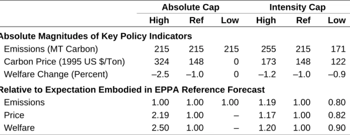
Results for Germany in 2010 are shown in Table 1.4
Over the period 1995-2010, average annual GDP growth rates for Germany in the high, reference and low cases are 3.7, 2.4 and 0.7%, respectively. The most important feature of the table is the change in outcomes relative to the “expected” values of key policy indicators. The expected or reference case values of these variables are identical for both types of emission limits; however, the variation in outcomes is much greater under the absolute cap than under its intensity-based counterpart. In the case of an absolute cap, emissions are fixed. But the amount of abatement and therefore the cost and the
4 EPPA’s reference scenario should not be interpreted to reflect the expectation of Germany’s negotiators at Kyoto
Table 1. EPPA Simulation of Quantity and Intensity Limits for Germany in 2010
Absolute Cap Intensity Cap
High Ref Low High Ref Low
Absolute Magnitudes of Key Policy Indicators
Emissions (MT Carbon) 215 215 215 255 215 171 Carbon Price (1995 US $/Ton) 324 148 0 173 148 122 Welfare Change (Percent) –2.5 –1.0 0 –1.2 –1.0 –0.9
Relative to Expectation Embodied in EPPA Reference Forecast
Emissions 1.00 1.00 1.00 1.19 1.00 0.80 Price 2.19 1.00 – 1.17 1.00 0.82 Welfare 2.50 1.00 – 1.20 1.00 0.90
reduction in welfare are more than twice as large if GDP growth is 25% higher than expected. With 25% lower GDP growth, all of these cost effects disappear since the Kyoto assigned amount exceeds Germany’s emissions and the cap is not binding.5 When an intensity limit is imposed, the same variations in GDP growth cause emissions to be higher or lower, but the changes in abatement cost and welfare differ from their respective reference or expected values by about 20%, significantly less variation than occurs with the absolute limit.6 These results are illustrative, but the underlying pattern is robust. Similar outcomes occur for different variations in GDP growth around some expectation, and for similar variations in GDP growth for other countries.
These results highlight an often-neglected feature of intensity limits, namely, that they are more demanding than absolute limits if actual GDP or output is less than expected. Most environmental regulations possess this feature: emission rate limits or technology mandates require the same level of control regardless of output.7 Thus, the presumption that intensity limits are inherently less stringent than absolute limits is erroneous. Whether an absolute cap or an equivalent intensity cap will be more demanding in any particular set of circumstances depends on actual outcomes relative to expectations at the time the limit is set.
3. A General Approach: Growth-Indexed Emission Limits
These results show that, when uncertainty is introduced, intensity-based and absolute emission caps have opposite effects. In fact, these two instruments are opposite limiting cases of a more
5 In the low growth scenario in which the emission limit is non-binding for Germany, emissions would be lower
except for leakage from other EU countries with binding limits in the low growth scenario.
6 Note that costs rise and fall with the variation in GDP. If intensity were invariant with respect to variations of
GDP, then costs stated per ton or on a percentage basis would remain constant. The positive, albeit greatly muted, correlation of per unit costs with GDP growth reflects the circumstance that the CO2 intensity of GDP is
also positively correlated with variations around reference growth rates.
7 Curiously, a frequent comment when we have presented this paper in the context of global GHG emission control
is that it seems unfair to require countries experiencing a recession to do as much as they would otherwise. This is, perhaps, an important consideration; but it does not find expression in most environmental regulation.
5
general, and flexible, emissions cap that combines the effect of a fixed emission limit, which we denote
t
Q , and a ceiling on emission intensity, t
t t ≡Q Y
γ , where Yt is expected GDP. We call this more general limit a growth-indexed emission limit, where the degree of indexing, or the relative weights of the two opposite forms, is determined by an indexing parameter, η, that can take any value between zero and one.8
The formula for the growth-indexed cap is:
(
)
t t tt Q Y
Q = 1−η +ηγ . (2)
This equation illustrates the limiting (in the mathematical sense) nature of absolute and intensity limits. An absolute cap corresponds to η = 0, in which case emissions at time t are determined solely by the fixed cap Qt, and intensity, γt (not γ ) will vary depending on Yt t. In the other
limiting case, η = 1, Qt disappears, the only operative constraint is the intensity limit, γ , andt the quantity of emissions depends solely on Yt. In this case, the cap on emissions is fully indexed
to fluctuations in GDP. When the indexing parameter takes values between the two extrema of zero and unity the absolute and intensity limits act jointly to determine the quantity of emissions in accordance with the weight given to each by η, or equivalently, to the extent that the cap adjusts to changes in GDP.9 Moreover, if an absolute or intensity limit at time t is established based on some earlier set of expectations and actual GDP is equal to expected GDP (Y =t Yt, as is the case under certainty) then the quantity of emissions is equal to the value of the absolute cap (Q =t Qt). This outcome holds for any value of η, implying that indexation is inconsequential
under either certainty or an accurate forecast of GDP. In the real world, indexation will matter and Qt will differ from Qtto the extent that the forecast is inaccurate.
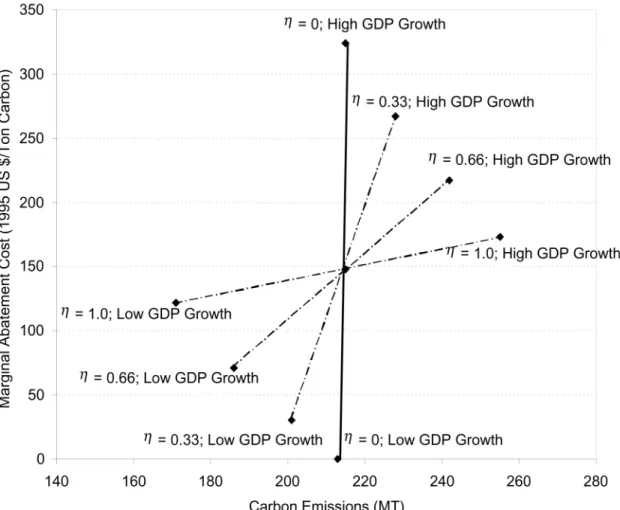
To illustrate the effects of differing degrees of indexation, we perform additional runs of the EPPA model in which the emission limits of the previous section were re-formulated as growth-indexed targets and imposed in the high and low GDP growth scenarios for differing values of indexation: η = 0, 0.33, 0.66, and 1. The results are shown in Figure 1, which plots the marginal cost of abatement and the level of emissions for Germany for different values of η. The solid vertical line represents outcomes for the absolute or zero-indexed cap in the three scenarios. The three dashed lines show the outcomes for caps with non-zero, positive indexing for the low and high growth scenarios. The lines for the indexing values of zero and unity plot the points that are given in the first two rows of Table 1. The other two lines are linear combinations in which the cap is allowed to vary by 33 and 66% (respectively) of the variation in GDP.
8 Technically, the growth-indexed cap is a convex combination of an intensity cap and an absolute emissions limit. 9
Allowances under a growth-indexed cap would have adjustable coverage or “redemption” values. Instead of always covering one ton of emissions, growth-indexed allowances of varying vintages would cover an amount of emissions that would depend upon the evolution of the index from some base period value. Thus, if output were expected to expand at g per cent per annum from some base period, t0, an allowance of vintage t would cover
(1 + g)t tons of the covered emissions. As shown in Table 1, the effect is to reduce the variance of future marginal cost of abatement. In practice, adjustment would occur with some lag.
Figure 1. Tradeoffs for Germany Between Abatement and Marginal Abatement Cost for Different Degrees of Growth Indexation of its Kyoto Cap
These results show that the indexing parameter adjusts the relative impacts of quantity or price effects, making possible any desired trade-off between the two over a broad range of outcomes. This leads to our third proposition, which is that if upside (or downside) fluctuations in costs are deemed undesirable, then the indexing parameter can be set to avoid as much of the undesired cost fluctuation as desired. The example presented here is for a single country, but it could as well represent a group of countries that trade emissions among themselves.10
4. Criteria for Choosing the Degree of Indexation
Given the trade-off identified in Figure 1, a relevant question is what criteria should guide the choice of emissions limit. The effects of indexation are similar to those resulting from the use of a price instead of a quantity instrument. On theoretical grounds, the choice depends on the rate at which marginal abatement costs and marginal damages rise with emissions (Weitzman, 1974). If marginal damages (or the benefits of abatement) rise steeply with emissions, then absolute limits
7
would be preferred. Conversely, if the marginal costs of abatement rise more steeply than marginal damages, which is the case with stock pollutants such as GHGs (see, e.g., Newell and Pizer, 2000), then an intensity-based cap, which in this case acts like a price instrument, would be preferred.
From a political economy standpoint, the degree of indexation reflects the tension inherent in the standard-setting process between positions that can be described as maintaining
environmental integrity and limiting economic growth. Those arguing for environmental
integrity tend to be attracted to absolute caps because of their ability to guarantee environmental outcomes.11
Those more concerned about the economy will view absolute caps as a “cap on growth”, or less dramatically, as leading to higher costs than anticipated if output is higher than expected.12
These latter concerns are typically cited in support of relative targets, such as in the relative sector of the U.K. Emissions Trading Scheme, and of a safety valve that would allow the absolute cap to be exceeded when marginal costs exceed some fee that is then paid for excess emissions (Jacoby and Ellerman, 2002; Morgenstern, 2002).
A more important concern on the international level may be the effect on the agreement to undertake common action. For instance, if parties agree upon some equitable allocation of a common burden under some set of shared expectations, how should variations from those expectations be handled? An absolute cap will result in the assignment of greater responsibility for achieving the common goal to those experiencing greater-than-expected growth in output, and in allocation of less responsibility to those experiencing less-than-expected output growth. Because GDP is a reflection of ability to pay, it could be argued that countries with greater-than-expected growth should abate more because of their good fortune, while less should be greater-than-expected from those with less than expected growth. Such an argument may also resonate with adherents to the non-economic notion that increased output is undesirable. For them, countries that enjoy larger increases in output should be required to incur higher abatement costs as some type of penalty or tax, and conversely, countries with smaller increases in output should do less as a reward for less growth. However appropriate this treatment on an international level, it is not commonly advocated for most environmental regulation on a sub-national level.
Whatever the rationale, the choice of an absolute cap presumes that the negotiating parties accept the implicit redistribution of the agreed-upon sharing of the common burden when their actual levels of GDP diverge from initial expectations, as they inevitably will. Without such acceptance, the consequent divergence in levels of abatement effort may lead to a breakdown
11 However, such attractiveness is often spurious, given the indirectness of the link between emissions and
environmental damage.
12 The link between caps and growth is as indirect, and potentially spurious, as the link between emissions and
environmental damages. Once the rhetoric is stripped away, appeals to “environmental integrity” and “caps on growth” are arguments about the effects, under uncertainty, of the choice of limit on emissions and costs.
of the initial agreement. This consideration is particularly important to the extent that the divergences from the expected paths of GDP growth are uncorrelated, which will cause some countries’ burdens to increase and others’ to diminish.13
Indexation may then be an attractive way of preserving the initial differentiation of burdens by automatically adjusting the required abatement to variations in growth.
5. Dynamic Properties
The discussion so far has been limited to the effects of the choice of emission limit in some single future period, but these effects apply equally in a multi-period context. Intensity caps can be as effective as absolute caps in reducing emissions over many periods. The primary differences would be that a series of absolute caps will exhibit more variation in year-to-year abatement and cost than a series of intensity caps and that cumulative emissions will be fixed for the former but not the latter.14 The frequent assertion that intensity caps cannot reduce emissions reflects a confusion concerning the form of the limit and the path of the desired emissions trajectory over time.
As with the misunderstanding about the voluntary and mandatory nature of absolute and intensity-based targets, this one seems to be associated with the Bush Administration’s setting of an intensity target for 2012 that is expected to allow emissions to increase in the interim. This target differs markedly from the expected 20 to 30% reduction of emissions that would have been required of the U.S. by the Kyoto Protocol. This difference concerns the magnitude of the initial step,
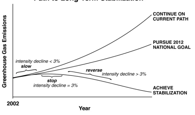
whether it should be big or modest, not the form of the limit. Neither the Kyoto Protocol nor the Bush Administration target for the U.S. makes any statement about what would come after 2012. The briefing materials accompanying President Bush’s adoption of an initially voluntary intensity target provide a suggestive picture, reproduced in Figure 2, of how emissions might be reduced over the longer run (White House, 2002). This “slow-stop-reverse” trajectory reduces emissions gradually from the expected, business-as-usual path at the beginning and the reduction intensifies as time goes on. In this figure, GDP is assumed to grow at 3% per annum and the slow, stop, and reverse phases occur where the policy-induced rates of decline in emission intensity are less than, equal to, and greater than the rate of GDP growth. As such, this figure illustrates the definitional requirement for an absolute reduction in the level of emissions: intensity must decline at a greater rate than the growth rate of GDP over the relevant period. This expected emissions profile is very
13 The potential disparity in effort among parties to the Kyoto Protocol is typically masked by the common practice
in modeling simulations of “high” and “low” scenarios that assumes that the economies of all parties grow more or less rapidly than in some reference case. To the extent that GDP growth is highly correlated across countries, then this consideration is less important since the required effort would be either more or less than expected for all. In addition, the variation in GDP that concerns us here is not the year-to-year fluctuation around some long-term trend but the shift in the realized long-long-term trend from what had been expected. A good example of this is the change in the trend of Japan’s GDP growth from the 1980s to the 1990s.
14 Banking would tend only to smooth the annual fluctuations in abatement and costs; in light of the foregoing
9
Figure 2. Slow-Stop-Reverse Emission Trajectory
different from that implied by the Kyoto Protocol and its presumed successors, but either trajectory could be achieved using a series of either absolute or intensity caps, or some combination thereof. The only differences would be in the variations of emissions and costs that would result from the choice of the limit and the deviation of actual outcomes from expectations at the time of the agreement. Whatever the magnitude of the initial step, the successive absolute or intensity caps extending over some relevant horizon would likely decline. The levels, timing, and rates of decline would be subject to negotiation and it is easy to see how the same considerations that governed the differentiation of the Kyoto targets would apply regardless of the form of the limit.15
Thus, our final proposition is that trajectories of either intensity-based targets or growth-indexed targets may be fashioned to achieve any desired path of GHG emissions.
A more important question may be whether the form of the limit has any effect on parties’ willingness to accept GHG emission limits or to agree to a long-term path of GHG emissions. Since an effective GHG control regime must be comprehensive and extend far into the future, a schedule of intensity limits that never reverses emissions growth is as ineffective as an ambitious initial reduction that is not achieved, or that leads to no further reductions in subsequent periods.
Given the history of the Kyoto Protocol, it is also pertinent to ask whether an absolute cap inhibits developing countries from agreeing to a limit in the first place and industrialized nations from agreeing to a limit for more than one period at a time—a procedure that is unlikely to lead to effective long-term control. All of the problems attendant on negotiating (and preserving)
long-term emission trajectories defined by absolute limits would be encountered with a schedule of maximum allowed emission intensity of GDP, except for one: the economic position of countries in the distant future. If the reluctance to accept an initial cap or to negotiate more than one step at a time in the Kyoto context reflects an unwillingness to agree to an absolute cap that might require more abatement effort in the future than a nation is currently willing to accept, a growth-indexed cap would solve this problem by automatically adjusting the cap upwards (or downwards) depending on the evolution of GDP. A nation could commit to limit and reduce GHG intensity by some amount, regardless of future GDP, instead of committing to an absolute level of future emissions that might be harder or easier to achieve than expected because of variations from expected GDP. And, of course, the choice is not restricted to these two limiting cases since they can be combined to whatever extent desired or appropriate.
6. Concluding Comments
These results provide no grounds for believing that the choice of the form of the emission limit will in and of itself lead to agreement on a binding limit on GHG emissions, much less an appropriate long-term trajectory, if countries are unwilling to undertake meaningful abatement. Nevertheless, intensity limits have the attractive property of lessening the importance of what is arguably the most significant imponderable for any nation considering the cost of GHG emission limits: future economic performance. To the extent that uncertainty about the effects of an absolute limit may impede agreement or cause existing agreements to unravel, then some degree of indexation to economic growth seems both desirable and necessary. Ultimately, the appropriate degree of indexation will be decided by political scientists and practicing negotiators as they weigh the relative merits of absolute and intensity-based caps, and the continuum of possible combinations thereof.
Although any departure from absolute caps is portrayed as antithetical to the Kyoto Protocol, it should be remembered that its breakdown, at least as initially envisaged, has led to calls for a wholly different approach to climate policy. Some would abandon entirely the targets-and-timetables architecture of the Kyoto Protocol and replace it with agreements on R&D
expenditure and technology transfer (Barrett, 2001) or with a global carbon tax (Cooper, 1998). In light of these demands, intensity limits are more compatible with the elements of the existing architecture discussed by Jacoby et al. (1998) than Kyoto’s politicized advocates may care to admit. A pure absolute cap is only the limiting form of a broad range of emission limitations in which the degree of indexing to GDP growth is a matter of choice. Perhaps, there should be no indexing; however, the widespread use of it in environmental regulation, including as an
instrument to reach the Kyoto caps by parties continuing to adhere to the Protocol, suggests that more attention should be paid to this variation than has been done in the past and certainly before abandoning the targets and timetables approach altogether.
11 References
1. Argentina (1999). Revision of the First National Communication to the U.N. Framework Convention on Climate Change, ARG/COM/2 B.
2. Barrett, S. (2001). “Towards a Better Climate Treaty.” AEI-Brookings Joint Center Opinion Piece, November 2001 (http://www.aei-brookings.org/policy/page.php?id=21).
3. Barros, V., and M. Conte Grand (2002). Implications of a Dynamic Target of Greenhouse Gas Emission Reduction: The Case of Argentina. Environment and Development Economics, 7(3): 547-569.
4. Cooper, R.N. (1998). Toward a Real Global Warming Treaty. Foreign Affairs, 77(2): 66-79. 5. Frankel, J. (1999). Greenhouse Gas Emissions. Bookings Institution Policy Brief No. 52,
Washington D.C.
6. Hahn, R.W., and R.N. Stavins (1999). What Has the Kyoto Protocol Wrought?: The Real Architecture of International Tradable Permit Markets. American Enterprise Institute Press: Washington, DC.
7. Jacoby, H.D., R.S. Eckaus, A.D. Ellerman, R.G. Prinn, D.M. Reiner and Z. Yang (1997). CO2 Emissions Limits: Economic Adjustments and the Distribution of Burdens. Energy
Journal, 18(3): 31-58.
8. Jacoby, H.D., R. Schmalensee and I. Sue Wing (1998). Toward a Useful Architecture for Climate Negotiations. OECD Workshop on the Economic Modeling of Climate Change, Paris, 17-18 September, pp. 283-306.
9. Jacoby, H.D., and A.D. Ellerman (2002). The Safety Valve and Climate Policy. MIT Joint Program on the Science and Policy of Global Change Report No. 83, Cambridge, MA. 10. Morgenstern, R. (2002). Reducing Carbon Emissions and Limiting Costs, in: U.S. Policy on
Climate Change: What Next?. Aspen Institute: Aspen, CO, pp. 165-176.
11. Newell, R.G., and W.A. Pizer (2000). Regulating Stock Externalities Under Uncertainty. Resources for the Future Discussion Paper 99–10–REV.
12. Reiner, D.M., and H.D. Jacoby (1997). Annex I Differentiation Proposals: Implications for Welfare, Equity and Policy. MIT Joint Program on the Science and Policy of Global Change Report No. 27, Cambridge, MA.
13. Weitzman, M.L. (1974) Prices vs. Quantities. Review of Economic Studies, 41(4): 477–491. 14. White House (2002). U.S. Climate Strategy: A New Approach. Policy Briefing Book,
REPORT SERIES of theMIT Joint Program on the Science and Policy of Global Change
1. Uncertainty in Climate Change Policy Analysis Jacoby & Prinn December 1994
2. Description and Validation of the MIT Version of the GISS 2D Model Sokolov & Stone June 1995
3. Responses of Primary Production and Carbon Storage to Changes in Climate and Atmospheric CO2 Concentration
Xiao et al. October 1995
4. Application of the Probabilistic Collocation Method for an Uncertainty Analysis Webster et al. January 1996 5. World Energy Consumption and CO2 Emissions: 1950-2050 Schmalensee et al. April 1996
6. The MIT Emission Prediction and Policy Analysis (EPPA) Model Yang et al. May 1996
7. Integrated Global System Model for Climate Policy Analysis Prinn et al. June 1996 (superseded by No. 36)
8. Relative Roles of Changes in CO2 and Climate to Equilibrium Responses of Net Primary Production and Carbon
Storage Xiao et al. June 1996
9. CO2 Emissions Limits: Economic Adjustments and the Distribution of Burdens Jacoby et al. July 1997
10. Modeling the Emissions of N2O & CH4 from the Terrestrial Biosphere to the Atmosphere Liu August 1996
11. Global Warming Projections: Sensitivity to Deep Ocean Mixing Sokolov & Stone September 1996
12. Net Primary Production of Ecosystems in China and its Equilibrium Responses to Climate Changes Xiao et al. Nov 1996 13. Greenhouse Policy Architectures and Institutions Schmalensee November 1996
14. What Does Stabilizing Greenhouse Gas Concentrations Mean? Jacoby et al. November 1996 15. Economic Assessment of CO2 Capture and Disposal Eckaus et al. December 1996
16. What Drives Deforestation in the Brazilian Amazon? Pfaff December 1996
17. A Flexible Climate Model For Use In Integrated Assessments Sokolov & Stone March 1997
18. Transient Climate Change & Potential Croplands of the World in the 21st Century Xiao et al. May 1997 19. Joint Implementation: Lessons from Title IV’s Voluntary Compliance Programs Atkeson June 1997
20. Parameterization of Urban Sub-grid Scale Processes in Global Atmospheric Chemistry Models Calbo et al. July 1997 21. Needed: A Realistic Strategy for Global Warming Jacoby, Prinn & Schmalensee August 1997
22. Same Science, Differing Policies; The Saga of Global Climate Change Skolnikoff August 1997
23. Uncertainty in the Oceanic Heat and Carbon Uptake & their Impact on Climate Projections Sokolov et al. Sept 1997 24. A Global Interactive Chemistry and Climate Model Wang, Prinn & Sokolov September 1997
25. Interactions Among Emissions, Atmospheric Chemistry and Climate Change Wang & Prinn September 1997 26. Necessary Conditions for Stabilization Agreements Yang & Jacoby October 1997
27. Annex I Differentiation Proposals: Implications for Welfare, Equity and Policy Reiner & Jacoby October 1997 28. Transient Climate Change & Net Ecosystem Production of the Terrestrial Biosphere Xiao et al. November 1997 29. Analysis of CO2 Emissions from Fossil Fuel in Korea: 1961−1994 Choi November 1997
30. Uncertainty in Future Carbon Emissions: A Preliminary Exploration Webster November 1997
31. Beyond Emissions Paths: Rethinking the Climate Impacts of Emissions Protocols Webster & Reiner November 1997 32. Kyoto’s Unfinished Business Jacoby, Prinn & Schmalensee June 1998
33. Economic Development and the Structure of the Demand for Commercial Energy Judson et al. April 1998
34. Combined Effects of Anthropogenic Emissions & Resultant Climatic Changes on Atmosph. OH Wang & Prinn April 1998 35. Impact of Emissions, Chemistry, and Climate on Atmospheric Carbon Monoxide Wang & Prinn April 1998
36. Integrated Global System Model for Climate Policy Assessment: Feedbacks and Sensitivity Studies Prinn et al. June 1998 37. Quantifying the Uncertainty in Climate Predictions Webster & Sokolov July 1998
38. Sequential Climate Decisions Under Uncertainty: An Integrated Framework Valverde et al. September 1998 39. Uncertainty in Atmospheric CO2 (Ocean Carbon Cycle Model Analysis) Holian October 1998 (superseded by No. 80)
40. Analysis of Post-Kyoto CO2 Emissions Trading Using Marginal Abatement Curves Ellerman & Decaux October 1998
41. The Effects on Developing Countries of the Kyoto Protocol & CO2 Emissions Trading Ellerman et al. November 1998
42. Obstacles to Global CO2 Trading: A Familiar Problem Ellerman November 1998
43. The Uses and Misuses of Technology Development as a Component of Climate Policy Jacoby November 1998 44. Primary Aluminum Production: Climate Policy, Emissions and Costs Harnisch et al. December 1998
45. Multi-Gas Assessment of the Kyoto Protocol Reilly et al. January 1999
46. From Science to Policy: The Science-Related Politics of Climate Change Policy in the U.S. Skolnikoff January 1999 47. Constraining Uncertainties in Climate Models Using Climate Change Detection Techniques Forest et al. April 1999 48. Adjusting to Policy Expectations in Climate Change Modeling Shackley et al. May 1999
49. Toward a Useful Architecture for Climate Change Negotiations Jacoby et al. May 1999
50. A Study of the Effects of Natural Fertility, Weather & Productive Inputs in Chinese Agriculture Eckaus & Tso July 1999 51. Japanese Nuclear Power and the Kyoto Agreement Babiker, Reilly & Ellerman August 1999
REPORT SERIES of theMIT Joint Program on the Science and Policy of Global Change
Contact the Joint Program Office to request a copy. The Report Series is distributed at no charge.
53. Developing Country Effects of Kyoto-Type Emissions Restrictions Babiker & Jacoby October 1999 54. Model Estimates of the Mass Balance of the Greenland and Antarctic Ice Sheets Bugnion October 1999 55. Changes in Sea-Level Associated with Modifications of Ice Sheets over 21st Century Bugnion October 1999 56. The Kyoto Protocol and Developing Countries Babiker, Reilly & Jacoby October 1999
57. Can EPA Regulate GHGs Before the Senate Ratifies the Kyoto Protocol? Bugnion & Reiner November 1999 58. Multiple Gas Control Under the Kyoto Agreement Reilly, Mayer & Harnisch March 2000
59. Supplementarity: An Invitation for Monopsony? Ellerman & Sue Wing April 2000
60. A Coupled Atmosphere-Ocean Model of Intermediate Complexity Kamenkovich et al. May 2000 61. Effects of Differentiating Climate Policy by Sector: A U.S. Example Babiker et al. May 2000
62. Constraining Climate Model Properties Using Optimal Fingerprint Detection Methods Forest et al. May 2000 63. Linking Local Air Pollution to Global Chemistry and Climate Mayer et al. June 2000
64. The Effects of Changing Consumption Patterns on the Costs of Emission Restrictions Lahiri et al. August 2000 65. Rethinking the Kyoto Emissions Targets Babiker & Eckaus August 2000
66. Fair Trade and Harmonization of Climate Change Policies in Europe Viguier September 2000
67. The Curious Role of “Learning” in Climate Policy: Should We Wait for More Data? Webster October 2000 68. How to Think About Human Influence on Climate Forest, Stone & Jacoby October 2000
69. Tradable Permits for GHG Emissions: A primer with reference to Europe Ellerman November 2000 70. Carbon Emissions and The Kyoto Commitment in the European Union Viguier et al. February 2001
71. The MIT Emissions Prediction and Policy Analysis (EPPA) Model: Revisions, Sensitivities, and Comparisons of
Results Babiker et al. February 2001
72. Cap and Trade Policies in the Presence of Monopoly and Distortionary Taxation Fullerton & Metcalf March 2001 73. Uncertainty Analysis of Global Climate Change Projections Webster et al. March 2001
74. The Welfare Costs of Hybrid Carbon Policies in the European Union Babiker et al. June 2001
75. Feedbacks Affecting the Response of the Thermohaline Circulation to Increasing CO2 Kamenkovich et al. July 2001
76. CO2 Abatement by Multi-fueled Electric Utilities: An Analysis Based on Japanese Data Ellerman & Tsukada July 2001
77. Comparing Greenhouse Gases Reilly, Babiker & Mayer July 2001
78. Quantifying Uncertainties in Climate System Properties using Recent Climate Observations Forest et al. July 2001 79. Uncertainty in Emissions Projections for Climate Models Webster et al. August 2001
80. Uncertainty in Atmospheric CO2 Predictions from a Parametric Uncertainty Analysis of a Global Ocean Carbon
Cycle Model Holian, Sokolov & Prinn September 2001
81. A Comparison of the Behavior of Different Atmosphere-Ocean GCMs in Transient Climate Change Experiments
Sokolov, Forest & Stone December 2001
82. The Evolution of a Climate Regime: Kyoto to Marrakech Babiker, Jacoby & Reiner February 2002 83. The “Safety Valve” and Climate Policy Jacoby & Ellerman February 2002
84. A Modeling Study on the Climate Impacts of Black Carbon Aerosols Wang March 2002 85. Tax Distortions and Global Climate Policy Babiker, Metcalf & Reilly May 2002
86. Incentive-based Approaches for Mitigating GHG Emissions: Issues and Prospects for India Gupta June 2002 87. Sensitivities of Deep-Ocean Heat Uptake and Heat Content to Surface Fluxes and Subgrid-Scale Parameters in an
Ocean GCM with Idealized Geometry Huang, Stone & Hill September 2002
88. The Deep-Ocean Heat Uptake in Transient Climate Change Huang et al. September 2002
89. Representing Energy Technologies in Top-down Economic Models using Bottom-up Information McFarland, Reilly
& Herzog October 2002
90. Ozone Effects on Net Primary Production and Carbon Sequestration in the Conterminous United States Using a Biogeochemistry Model Felzer et al. November 2002
91. Exclusionary Manipulation of Carbon Permit Markets: A Laboratory Test Carlén November 2002
92. An Issue of Permanence: Assessing the Effectiveness of Temporary Carbon Storage Herzog et al. December 2002 93. Is International Emissions Trading Always Beneficial? Babiker et al. December 2002
94. Modeling Non-CO2 Greenhouse Gas Abatement Hyman et al. December 2002
95. Uncertainty Analysis of Climate Change and Policy Response Webster et al. December 2002 96. Market Power in International Carbon Emissions Trading: A Laboratory Test Carlén January 2003
97. Emissions Trading to Reduce GHG Emissions in the US: The McCain-Lieberman Proposal Paltsev et al. June 2003 98. Russia’s Role in the Kyoto Protocol Bernard et al. June 2003
99. Thermohaline Circulation Stability: A Box Model Study Lucarini & Stone June 2003 100. Absolute vs. Intensity-Based Emissions Caps Ellerman & Sue Wing July 2003