Algorithms and Applications for Gaussian Graphical
Models under the Multivariate Totally Positive
Constraint of Order 2
by
Uma Roy
Submitted to the Department of Electrical Engineering and Computer
Science
in partial fulfillment of the requirements for the degree of
Master of Engineering in Electrical Engineering and Computer Science
at the
MASSACHUSETTS INSTITUTE OF TECHNOLOGY
June 2019
c
○ Massachusetts Institute of Technology 2019. All rights reserved.
Author . . . .
Department of Electrical Engineering and Computer Science
May 22, 2019
Certified by . . . .
Caroline Uhler
Associate Professor
Thesis Supervisor
Accepted by . . . .
Katrina LaCurts
Chair, Master of Engineering Thesis Committee
Algorithms and Applications for Gaussian Graphical Models
under the Multivariate Totally Positive Constraint of Order 2
by
Uma Roy
Submitted to the Department of Electrical Engineering and Computer Science on May 22, 2019, in partial fulfillment of the
requirements for the degree of
Master of Engineering in Electrical Engineering and Computer Science
Abstract
We consider the problem of estimating an undirected Gaussian graphical model when the underlying distribution is multivariate totally positive of order 2 (MTP2), a strong
form of positive dependence. A large body of methods have been proposed for learning undirected graphical models without the MTP2 constraint. A major limitation of these
methods is that their consistency guarantees in the high-dimensional setting usually require a particular choice of a tuning parameter, which is unknown a priori in real world applications. We show that an undirected graphical model under MTP2 can be
learned consistently without any tuning parameters. We evaluate this new estimator on synthetic and real-world financial data sets, showing that it out-performs other methods in the literature with tuning parameters. We further explore applications of estimators in the MTP2 setting to covariance estimation for finance. In particular, the
very well-explored optimal Markowitz portfolio allocation problem requires a precise estimate of the covariance matrix of returns. By exploiting the fact that the returns of assets are typically positively dependent, we propose a new estimator based on MTP2 estimation and show that this estimator outperforms (in terms of out-of-sample
risk) baseline methods including shrinkage techniques and explicitly providing market factors on stock-market data spanning over thirty years.
Thesis Supervisor: Caroline Uhler Title: Associate Professor
Acknowledgments
First and foremost I would like to thank my advisor Professor Caroline Uhler for the mentorship, guidance and help she provided this year; I cannot imagine a better advisor. Caroline’s good spirit is infectious. Every time I talked to her this year, I left in a better mood thinking that all problems were solvable. I would also like to thank Yuhao Wang, another graduate student in Professor Uhler’s lab, with whom I collaborated very closely on the tuning-parameter free algorithm for estimation under MTP2. In particular, the proof of the consistency of this algorithm should be credited
to him. Yuhao was a pleasure to work with throughout this project and I learned a lot about statistics and mathematics under his guidance. I would also like to thank Raj Agrawal, another graduate student in Caroline’s lab, with whom I collaborated on the applications of MTP2 estimation to covariance estimation in finance. Raj was
also a pleasure to work with and I learned a lot about experimental design from him. I would also like to thank the entire Uhler lab for being a wonderful and supportive community of students who made my masters experience better.
I would also like to thank my many friends at MIT for making the past year (and the past four years) some of the best of my life. And finally, I would like to thank my family for supporting me and encouraging me from a young age. I feel very privileged to have parents who pushed me and fostered my love for mathematics. Without them, I would not have had any of the wonderful opportunities that I am lucky to have today. Finally, I dedicate this thesis to my brother, Vedant Roy. Thank you for being the best little brother I could have ever imagined. Your creativity, intelligence and thoughtful attitude towards life inspire me constantly. You are wise beyond your years and I am lucky to be your older sister.
Contents
1 Learning High-Dimensional Gaussian Graphical Models under Total
Positivity without Tuning Parameters 13
1.1 Introduction . . . 13
1.2 Preliminaries and Related Work . . . 15
1.3 Algorithm and Consistency Guarantees . . . 17
1.4 Empirical Evaluation . . . 22
1.4.1 Synthetic Data . . . 22
1.4.2 Application to Financial Data . . . 25
1.5 Discussion . . . 27
2 Covariance Matrix Estimation under Total Positivity for Portfolio Selection 29 2.1 Introduction . . . 29
2.2 Background . . . 32
2.2.1 Notation . . . 32
2.2.2 Global Minimum Variance Portfolio . . . 33
2.2.3 Covariance estimators . . . 34
2.2.4 Factor Models . . . 34
2.2.5 Covariance Estimators for Factor Models . . . 36
2.2.6 Shrinkage of eigenvalues . . . 37
2.2.7 𝐿1 Regularization of the Precision Matrix . . . 38
2.3 MTP2 and our Method . . . 39
2.3.2 Multivariate Gaussian Returns . . . 42
2.3.3 Future Work: Accommodating Heavy-Tailed Returns Data . . 44
2.4 Results . . . 45
2.4.1 Methodology . . . 45
2.4.2 Metrics . . . 46
2.4.3 Comparison of various estimators of the GMV portfolio . . . . 47
2.4.4 Momentum Evaluation . . . 47
2.4.5 MTP2 vs. other methods discussion . . . 50
2.5 Conclusion . . . 50
A Learning High-Dimensional Gaussian Graphical Models under Total Positivity without Tuning Parameters 53 A.1 Proof of Lemma 1.3.7 . . . 53
A.1.1 Characterization of maximal overlaps . . . 53
A.1.2 Proof of Lemma 1.3.7 . . . 54
A.2 Proof of Theorem 1.3.6 . . . 60
A.3 Proof of Theorem 1.3.5 . . . 61
A.4 Further Comments on Empirical Evaluation . . . 63
A.4.1 Stability Selection . . . 63
A.4.2 ROC Curves . . . 64
List of Figures
1-1 Comparison of different algorithms evaluated on MCC across (a)
ran-dom, (b) chain and (c) grid graphs with 𝑝 = 100 and 𝑁 ∈ {25, 50, 100, 200, 500, 1000}. For each choice of 𝑝, 𝑁 for a given graph, results are shown as an average
across 20 replications. . . 24 1-2 (a) ROC curves, (b) MCC, and (c) true positive rate versus normalized
tuning parameter for random graphs with 𝑝 = 100 and 𝑁 = 500 across 30 trials. The shaded regions correspond to ±1 standard deviation of MCC (TPR resp.) across 30 trials. . . 25 2-1 The sample correlation matrix of global stock markets taken from 2016
daily returns. Notice that the covariance matrix contains all positive entries and the precious matrix is an M-matrix which implies that the joint distribution is MTP2 (see Section 2.3.2 for details). . . 31
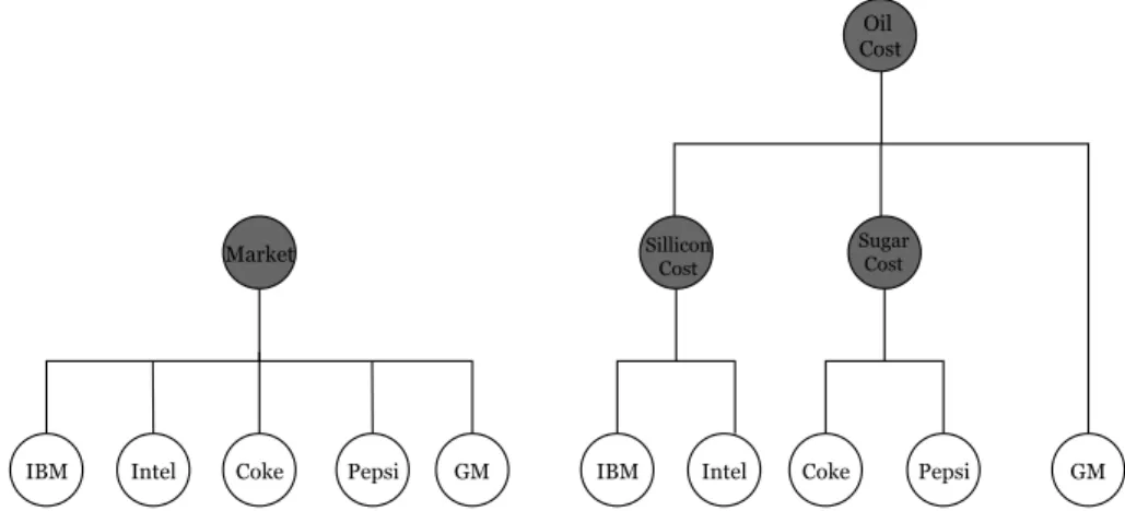
2-2 Shaded nodes represent factors that are potentially unobserved, and unshaded nodes are the observed returns of different companies. The left hand figure represents a simple model where we think the market drives the returns of all stocks as in CAPM. The right hand figure represents a more complicated latent tree where we believe that there are latent sector-level factors driving the returns of different assets. . 42 A-1 ROC curves for 𝑁 = 50, 100, 200 respectively averaged across 30 trials
List of Tables
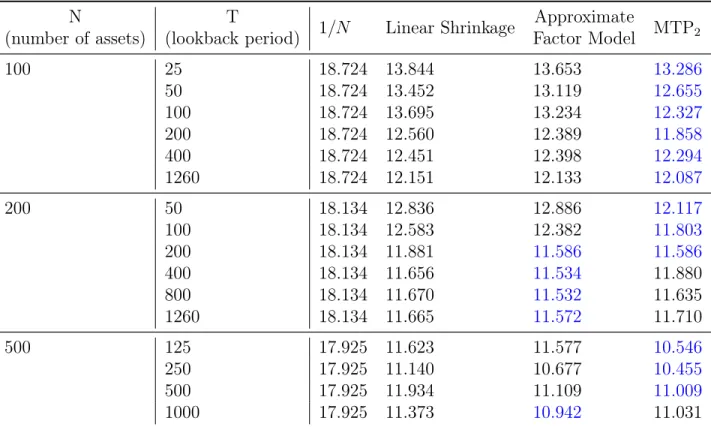
1.1 Modularity scores of the estimated graphs; higher score indicates better clustering performance. For our algorithm we used the theoretically optimal value of 𝛾 = 7/9. . . 26 2.1 Performance of different estimators for various 𝑁 (number of assets) and
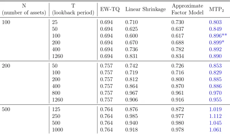
𝑇 (number of samples considered). For each combination of 𝑁, 𝑇 and choice of estimator, the number in the table is the standard deviation of the returns of the portfolio given by applying the estimator to the rolling out of sample. . . 48 2.2 Performance of different estimators for various 𝑁 (number of assets)
and 𝑇 (number of samples considered). For each combination of 𝑁, 𝑇 and choice of estimator, the number in the table is the information ratio (ratio of the average return to the standard deviation of returns) of the portfolio given by applying the estimator to the rolling out of sample. . . 49
Chapter 1
Learning High-Dimensional Gaussian
Graphical Models under Total
Positivity without Tuning Parameters
1.1
Introduction
Gaining insights into complex phenomena often requires characterizing the relationships among a large number of variables. Gaussian graphical models offer a powerful framework for representing high-dimensional distributions by capturing the conditional dependencies between the variables of interest in the form of a network. These models have been extensively used in a wide variety of domains ranging from speech recognition [37] to genomics [43] and finance [68].
In this section we consider the problem of learning a Gaussian graphical model under the constraint that the distribution is multivariate totally positive of order 2 (MTP2),
or equivalently, that all partial correlations are non-negative. Such models are also known as attractive Gaussian random fields. MTP2 was first studied in [7, 27, 40, 41]
and later also in the context of graphical models [20, 45]. MTP2 is a strong form of
positive dependence, which is relevant for modeling in various applications including phylogenetics or portfolio selection, where the shared ancestry or latent global market
variable often lead to positive dependence among the observed variables [59, 71]. Due to the explosion of data where the number of variables 𝑝 is comparable to or larger than the number of samples 𝑛, the problem of learning undirected Gaussian graphical models in the high-dimensional setting has been a central topic in machine learning, statistics and optimization. There are two main classes of algorithms for structure estimation for Gaussian graphical models in the high-dimensional setting. A first class of algorithms attempts to explicitly recover which edges exist in the graphical model, for example using conditional independence tests [1, 65] or neighborhood selection [56]. A second class of algorithms instead focuses on estimating the precision matrix. The most prominent of these algorithms is graphical lasso [29, 61], which applies an ℓ1 penalty to the log-likelihood function to estimate the precision matrix.
Other algorithms include moment-matching approaches such as CLIME [8, 9] as well as optimization with non-convex penalties [25, 44, 51]. The main limitation of all aforementioned approaches is the requirement of a specific tuning parameter to obtain consistency guarantees in estimating the edges of the underlying graphical model. In most real-world applications, the correct tuning parameter is unknown and difficult to discover.
The algorithms described above are for learning the underlying undirected graph in general Gaussian models. In this section, we consider the special setting of MTP2
Gaussian models. Several algorithms have been proposed that are able to exploit the additional structure imposed by MTP2 with the goal of obtaining stronger results than
for general Gaussian graphical models. In particular, [45] showed that the MLE exists whenever the sample size 𝑁 > 2 (independent of the number of variables 𝑝), which is striking given that 𝑁 > 𝑝 is required for the MLE to exist in general Gaussian graphical models. Since the MLE under MTP2 is not a consistent estimator for the
structure of the graph, [63] considered applying thresholding to entries in the MLE, but this procedure requires a tuning parameter and does not have consistency guarantees.
The three main contributions of this section are: 1) we provide a new algorithm for learning Gaussian graphical models under MTP2 that is based on conditional
algorithm is consistent in the high-dimensional setting without the need of a particular choice of tuning parameter; 3) we show that our algorithm compares favorably to other methods for learning graphical models on both simulated data and financial data.
1.2
Preliminaries and Related Work
Gaussian graphical models: Given a graph 𝐺 = ([𝑝], ℰ ) with vertex set [𝑝] = {1, · · · , 𝑝} and edge set ℰ we associate to each node 𝑖 in 𝐺 a random variable 𝑋𝑖. A
distribution P on the nodes [𝑝] forms an undirected graphical model with respect to 𝐺 if
𝑋𝑖 ⊥⊥ 𝑋𝑗 | 𝑋[𝑝]∖{𝑖,𝑗} for all (𝑖, 𝑗) /∈ 𝐸. (1.1)
When P is Gaussian with covariance matrix Σ and precision matrix Θ := Σ−1, the setting we concentrate on in this section, then (1.1) is equivalent to Θ𝑖𝑗 = 0 for all
(𝑖, 𝑗) /∈ 𝐸. By the Hammersley-Clifford Theorem, for strictly positive densities such as the Gaussian, (1.1) is equivalent to
𝑋𝑖 ⊥⊥ 𝑋𝑗 | 𝑋𝑆 for all 𝑆 ⊆ [𝑝] ∖ {𝑖, 𝑗} that separate 𝑖, 𝑗,
where 𝑖, 𝑗 are separated by 𝑆 in 𝐺 when 𝑖 and 𝑗 are in different connected components of 𝐺 after removing the nodes 𝑆 from 𝐺. In the Gaussian setting 𝑋𝑖 ⊥⊥ 𝑋𝑗 | 𝑋𝑆 if
and only if the corresponding partial correlation coefficient 𝜌𝑖𝑗|𝑆 is zero, which can be
calculated from submatrices of Σ, namely
𝜌𝑖𝑗|𝑆 = −
((Σ𝑀,𝑀)−1)𝑖,𝑗
√︀((Σ𝑀,𝑀)−1)𝑖,𝑖((Σ𝑀,𝑀)−1)𝑗,𝑗
, where 𝑀 = 𝑆 ∪ {𝑖, 𝑗}.
MTP2 distributions: A density function 𝑓 on R𝑝 is MTP 2 if
where ∨, ∧ denote the coordinate-wise minimum and maximum respectively [27, 40]. In particular, a Gaussian distribution is MTP2 if and only if its precision matrix Θ is
an 𝑀 -matrix, i.e. Θ𝑖𝑗 ≤ 0 for all 𝑖 ̸= 𝑗 [7, 41]. This implies that all partial correlation
coefficients are non-negative, i.e., 𝜌𝑖𝑗|𝑆 ≥ 0 for all 𝑖, 𝑗, 𝑆 [41]. In addition, for MTP2
distributions it holds that 𝑋𝑖 ⊥⊥ 𝑋𝑗 | 𝑋𝑆 if and only if 𝑖, 𝑗 are separated in 𝐺 given
𝑆 [20]. Hence 𝑖, 𝑗 are connected in 𝐺 given 𝑆 if and only if 𝜌𝑖𝑗|𝑆 > 0.
Algorithms for learning Gaussian graphical models: We say that an algorithm is consistent if the non-zero entries of its estimated precision matrix correspond to edges in the underlying graph 𝐺. CMIT, an algorithm proposed in [1], is most related to the approach in this section. Starting in the complete graph, edge (𝑖, 𝑗) is removed if there exists 𝑆 ⊆ [𝑝] ∖ {𝑖, 𝑗} with 𝑆 ≤ 𝜂 (for a tuning parameter 𝜂 that represents the maximum degree of the underlying graph) such that the corresponding empirical partial correlation coefficient satisfies | ˆ𝜌𝑖𝑗|𝑆| ≤ 𝜆𝑁,𝑝. For consistent estimation, the
tuning parameter 𝜆𝑁,𝑝 needs to be selected carefully depending on the sample size
𝑁 and number of nodes 𝑝. Intuitively, if (𝑖, 𝑗) /∈ 𝐺, then 𝜌𝑖𝑗|𝑆 = 0 for all 𝑆 that
separate (𝑖, 𝑗). Since ˆ𝜌𝑖𝑗|𝑆 concentrates around 𝜌𝑖𝑗|𝑆, it holds with high probability
that there exists 𝑆 ⊆ [𝑝] ∖ {𝑖, 𝑗} for which | ˆ𝜌𝑖𝑗|𝑆| ≤ 𝜆𝑁,𝑝, so that edge (𝑖, 𝑗) is removed
from 𝐺. Other estimators such as graphical lasso [61] and neighborhood selection [56] also require a tuning parameter: 𝜆𝑁,𝑝 represents the coefficient of the ℓ1 penalty and
critically depends on 𝑁 , 𝑝 for consistent estimation. Finally, with respect to estimation specifically under the MTP2 constraint, the authors in [63] propose thresholding the
MLE ̂︀Ω of the precision matrix, which can be obtained by solving the following convex optimization problem:
̂︀
Ω := min
Ω⪰0, Ω𝑖𝑗≤0 ∀𝑖̸=𝑗
− log det(Ω) + trace(Ω ˆΣ), (1.2)
where ˆΣ is the sample covariance matrix. The threshold quantile 𝑞 is a tuning parameter, and apart from empirical evidence that thresholding works well, there are no known theoretical consistency guarantees for this procedure.
In addition to relying on a specific tuning parameter for consistent estimation, exist-ing estimators require additional conditions with respect to the underlyexist-ing distribution. The consistency guarantees of graphical lasso [61] and moment matching approaches such as CLIME [8] require that the diagonal elements of Σ are upper bounded by a constant and that the minimum edge weight min𝑖̸=𝑗,Θ𝑖𝑗̸=0|Θ𝑖𝑗| ≥ 𝐶√︀log(𝑝)/𝑁 for
some positive constant 𝐶. Consistency of CMIT [1] also requires the minimum edge weight condition. Consistency of CLIME requires a bounded matrix 𝐿1 norm of the
precision matrix Θ, which implies that all diagonal elements of Θ are bounded.
1.3
Algorithm and Consistency Guarantees
Algorithm 1 is our proposed procedure for learning a Gaussian graphical model under the MTP2 constraint. In the following, we first describe Algorithm 1 in detail and
then prove its consistency without the need of any tuning parameter.
Similar to CMIT [1], Algorithm 1 starts with the fully connected graph ˆ𝐺 and sequentially removes edges based on conditional independence tests. The algorithm
Algorithm 1 Structure learning under total positivity without tuning parameter Input: Matrix of observations ˆ𝑋 ∈ R𝑁 ×𝑝 with sample size 𝑁 on 𝑝 nodes.
Output: Estimated graph ˆ𝐺.
1: Set ˆ𝐺 as the completely connected graph over the vertex set [𝑝]; set ℓ := −1;
2: repeat
3: set ℓ = ℓ + 1;
4: repeat
5: select a (new) ordered pair (𝑖, 𝑗) that are adjacent in ˆ𝐺 and such that |adj𝑖( ˆ𝐺) ∖ {𝑗}| ≥ ℓ;
6: repeat
7: choose a (new) subset 𝑆 ⊆ adj𝑖( ˆ𝐺) ∖ {𝑗} with |𝑆| = ℓ and then choose a (new) node 𝑘 ∈ [𝑝] ∖ 𝑆 ∪ {𝑖, 𝑗};
8: calculate the empirical partial coefficient ˆ𝜌𝑖𝑗|𝑆∪{𝑘} using randomly drawn
data with batch size 𝑀 := 𝑁𝛾; if ˆ𝜌𝑖𝑗|𝑆∪{𝑘} < 0, delete 𝑖 − 𝑗 from ˆ𝐺;
9: until edge 𝑖 − 𝑗 is deleted from ˆ𝐺 or all 𝑆 and 𝑘 are considered;
10: until all ordered pairs 𝑖, 𝑗 that are adjacent in ˆ𝐺 with |adj𝑖( ˆ𝐺) ∖ {𝑗}| ≥ ℓ are considered;
iterates with respect to a parameter ℓ that starts at ℓ = 0. In each iteration, for all pairs of nodes 𝑖, 𝑗 such that the edge (𝑖, 𝑗) ∈ ˆ𝐺 and node 𝑖 has at least ℓ neighbors (denoted by adj𝑖( ˆ𝐺)), the algorithm considers all combinations of subsets 𝑆 of adj𝑖( ˆ𝐺)
excluding 𝑗 that have size ℓ and all nodes 𝑘 ̸= 𝑖, 𝑗 that are not in 𝑆. For each combination of subset 𝑆 and node 𝑘, it calculates the empirical partial correlation coefficient ˆ𝜌𝑖𝑗|𝑆∪{𝑘}. Importantly, ˆ𝜌𝑖𝑗|𝑆∪{𝑘} is calculated only on a subset (which we
refer to as a batch) of size 𝑀 := 𝑁𝛾 that we draw randomly from the 𝑁 samples. If any of these empirical partial correlation coefficients are negative, then edge 𝑖 − 𝑗 is deleted from ˆ𝐺 (and no further tests are performed on (𝑖, 𝑗)). Each iteration of the algorithm increases ℓ by 1 and the algorithm terminates when for all nodes 𝑖, 𝑗 such that (𝑖, 𝑗) ∈ ˆ𝐺, the neighborhood of 𝑖 excluding 𝑗 has size strictly less than ℓ.
The basic intuition behind Algorithm 1 is that if there is an edge 𝑖 − 𝑗 in 𝐺, then all partial correlations 𝜌𝑖𝑗|𝑆 are positive because of the basic properties of MTP2. In
the limit of large 𝑁 , this implies that all ˆ𝜌𝑖𝑗|𝑆 are positive. On the other hand, when
𝑖 and 𝑗 are not connected in the true underlying graph, then there exists a list of conditioning sets 𝑆1, · · · , 𝑆𝐾 such that 𝜌𝑖𝑗|𝑆𝑘 = 0 for all 1 ≤ 𝑘 ≤ 𝐾. When 𝐾 is large
enough, then intuitively there should exist 1 ≤ 𝑘 ≤ 𝐾 such that ˆ𝜌𝑖𝑗|𝑆𝑘 < 0 with high
probability. However, since for overlapping conditioning sets the empirical partial correlations are highly correlated, we use separate batches of data for their estimation. This leads to a procedure for learning the underlying Gaussian graphical model by deleting edges based on the signs of empirical partial correlation coefficients.
Having provided the high level intuition behind Algorithm 1, we now prove its consistency under common assumptions on the underlying data generating process. Let 𝑑 denote the maximum degree of the true underlying graph 𝐺. For any positive semidefinite matrix 𝐴, let 𝜆min(𝐴) and 𝜆max(𝐴) denote the minimum and maximum
eigenvalues of 𝐴 respectively.
Condition 1.3.1. There exist positive constants 𝜎min and 𝜎max such that for any
subset of nodes 𝑆 ⊆ [𝑝] with |𝑆| ≤ 𝑑 + 4, the true underlying covariance matrix satisfies
Note that since 𝜆max(Σ𝑆) ≤ trace(Σ𝑆) and |𝑆| ≤ 𝑑 + 4, it is straightforward to
show that a sufficient condition for 𝜆max(Σ𝑆) ≤ 𝜎max is that all diagonal entries of
Σ scale as a constant. This condition is also required by many existing methods including graphical lasso and CLIME; see Section 1.2. Similarly, a sufficient condition for 𝜆min(Σ𝑆) ≥ 𝜎min is that all diagonal entries of Θ scale as a constant, which is also
required by CLIME.
Condition 1.3.2. There exists a positive constant 𝑐𝜌 such that for any two nodes
𝑖, 𝑗 ∈ [𝑝], if (𝑖, 𝑗) ∈ 𝐺, then 𝜌𝑖,𝑗|[𝑝]∖{𝑖,𝑗} ≥ 𝑐𝜌
√︀
(log 𝑝)/(𝑁3/4).
Condition 1.3.2 is a standard condition for controlling the minimum edge weight in 𝐺 as required, for example, by graphical lasso. While the minimum threshold in our condition scales as √︀(log 𝑝)/(𝑁3/4), graphical lasso only requires √︀(log 𝑝)/𝑁
(but instead requires a particular choice of tuning parameter and the incoherence condition).
Condition 1.3.3. The size of 𝑝 satisfies that 𝑝 ≥ 𝑁18 + 𝑑 + 2.
Condition 1.3.3 implies that the high-dimensional consistency guarantees of Algo-rithm 1 cannot be directly generalized to the low-dimensional setting where 𝑝 scales as a constant. We now provide the main result of our section, namely consistency of Algorithm 1.
Theorem 1.3.4. Assuming that the maximum neighbourhood size 𝑑 scales as a con-stant and under conditions 1.3.1-1.3.3 with 𝑐𝜌 sufficiently large, then for any 𝛾 ∈ (34, 1)
there exist positive constants 𝜏 and 𝐶 that depend on (𝑐𝜌, 𝜎max, 𝜎min, 𝑑, 𝛾) such that
with probability at least 1 − 𝑝−𝜏− 𝑝2𝑒−𝐶𝑁1−𝛾2 ∧(4𝛾−3)
, the graph estimated by Algorithm 1 is the same as the underlying graph 𝐺.
Remark 1.3.1. Although in practice the choice of 𝛾 can “act like" a tuning parameter (see Section 1.4), it is fundamentally different from a tuning parameter in the traditional sense, since the consistency guarantees of our algorithm hold for any 𝛾 ∈ (34, 1). Note that this is in contrast to the other methods outlined in Section 1.2, where the consistency guarantees require a specific choice of the tuning parameter in the
algorithm, which is unknown a priori. By setting 1−𝛾2 = (4𝛾 − 3), we obtain that the theoretically optimal value is 𝛾 = 7/9, as this leads to the best asymptotic rate. However, as seen in Section 1.4, in practice different values of 𝛾 can lead to different results. In particular, higher values of 𝛾 empirically lead to removing less edges since the overlap between batches is higher and thus the empirical partial correlation coefficients are more correlated with each other.
Proof of Theorem 1.3.4: In the following, we provide an overview of the proof of our main result. Theorems 1.3.5 and 1.3.6 show that at iteration ℓ = 𝑑 + 1, the graph ˆ𝐺 estimated by Algorithm 1 is exactly the same as the underlying graph 𝐺. The proof is then completed by showing that Algorithm 1 stops exactly at iteration ℓ = 𝑑 + 1. All proofs are provided in Appendix A.
We start with Theorem 1.3.5, which bounds the false negative rate of Algorithm 1, i.e. showing that all edges (𝑖, 𝑗) in the true graph 𝐺 are retained.
Theorem 1.3.5 (False negative rate). Under Conditions 1.3.1 and 1.3.2 and 𝑐𝜌
sufficiently large, there exists a positive constant 𝜏 that depends on (𝑐𝜌, 𝜎max, 𝜎min, 𝑑)
such that with probability at least 1 − 𝑝−𝜏, the graph ˆ𝐺 estimated by Algorithm 1 at iteration ℓ = 𝑑 + 1 contains all edges (𝑖, 𝑗) ∈ 𝐺.
The proof of Theorem 1.3.5 is based on concentration inequalities in estimating partial correlation coefficients. The high-level intuition behind the proof is that because the empirical partial correlation coefficients concentrate exponentially around the true partial correlation coefficients, then with high probability if an edge exists, no empirical partial correlation coefficient will be negative; as a consequence, Algorithm 1 will not eliminate the edge.
The following theorem bounds the false positive rate; namely, it shows that with high probability Algorithm 1 will delete all edges (𝑖, 𝑗) that are not in the true graph 𝐺.
Theorem 1.3.6 (False positive rate). Under Conditions 1.3.1 and 1.3.3, there exists a positive constant 𝐶 that depends on (𝜎max, 𝜎min, 𝑑), 𝛾) such that with probability at
least 1 − 𝑝2𝑒−𝐶1−𝛾2 ∧4𝛾−3, the graph ˆ𝐺 estimated by Algorithm 1 at iteration ℓ = 𝑑 + 1
does not contain any edges (𝑖, 𝑗) /∈ 𝐺.
The proof of Theorem 1.3.6 relies heavily on the following lemma that considers the orthant probability of partial correlation coefficients. Recall in Algorithm 1 that for a particular edge 𝑖 − 𝑗 in the estimated graph ˆ𝐺 at a given iteration, we calculate a series of empirical partial correlation coefficients with different conditioning sets. The only way Algorithm 1 will not delete the edge is if all empirical partial correlation coefficients are ≥ 0. Thus given 2 nodes 𝑖, 𝑗 for which (𝑖, 𝑗) /∈ 𝐺, we need to upper bound the orthant probability that all empirical partial correlation coefficients computed by Algorithm 1 are non-negative. As we will discuss next, the use of batches is critical for this result.
Lemma 1.3.7. Consider a pair of nodes (𝑖, 𝑗) /∈ 𝐺. Assume that there exists 𝐾 := 𝑁1−𝛾2 sets of nodes 𝑆1, · · · , 𝑆𝐾 ⊆ [𝑝] ∖ {𝑖, 𝑗} with |𝑆𝑘| ≤ 𝑑 + 2 that satisfy 𝜌𝑖𝑗|𝑆
𝑘 = 0.
Then there exists a positive constant 𝐶 that depends on (𝜎max, 𝜎min, 𝑑) such that
Pr( ˆ𝜌𝑖𝑗|𝑆𝑘 > 0 ∀𝑘 ∈ [𝐾]) ≤ exp(−𝐶𝑁 1−𝛾
2 ∧4𝛾−3). (1.3)
To provide intuition for the proof of Lemma 1.3.7, consider a scenario where the batch size 𝑀 is chosen small enough such that the batches used to estimate the different ˆ𝜌𝑖𝑗|𝑆𝑘’s have no overlap. Since in this case all ˆ𝜌𝑖𝑗|𝑆𝑘’s are independent, the
bound in Lemma 1.3.7 can easily be proven, namely:
Pr( ˆ𝜌𝑖𝑗|𝑆𝑘 > 0 ∀𝑘 ∈ [𝐾]) = 𝐾 ∏︁ 𝑘=1 Pr( ˆ𝜌𝑖𝑗|𝑆𝑘 > 0) = (︁1 2 )︁𝐾 = exp(−(log 2) · 𝑁1−𝛾2 ).
However, for small batch size 𝑀 the empirical partial correlation coefficients ˆ𝜌𝑖𝑗|𝑆
don’t concentrate around 𝜌𝑖𝑗|𝑆, which may result in false negatives. In the proof of
Lemma 1.3.7 we show that choosing a batch size of 𝑀 = 𝑁𝛾 guarantees the required
concentration result as well as a sufficiently weak dependence among the empirical partial correlation coefficients ˆ𝜌𝑖𝑗|𝑆𝑘’s to obtain the exponential upper bound in (1.3)
control over all edges (𝑖, 𝑗) ̸∈ 𝐺. Finally, to complete the proof of Theorem 1.3.4, it remains to show that Algorithm 1 terminates at iteration ℓ = 𝑑 + 1.
Proof of Theorem 1.3.4. It follows from Theorem 1.3.5 and Theorem 1.3.6 that with probability at least 1 − 𝑝−𝜏 − 𝑝2𝑒−𝐶𝑁1−𝛾2 ∧4𝛾−3
, the graph estimated by Algorithm 1 at iteration ℓ = 𝑑 + 1 is exactly the same as 𝐺. Since the maximum degree of 𝐺 is at most 𝑑, it matches the stopping criterion of Algorithm 1. As a consequence, Algorithm 1 terminates at iteration ℓ = 𝑑 + 1.
1.4
Empirical Evaluation
In the following section, we evaluate the performance of our algorithm for structure recovery in MTP2 Gaussian graphical models in the high-dimensional, sparse regime.
We first compare the performance of Algorithm 1 to various other methods on syntheti-cally generated datasets and then present an application to graphical model estimation on financial data.
1.4.1
Synthetic Data
Given a precision matrix Θ ∈ R𝑝×𝑝, we generate 𝑁 i.i.d. samples 𝑥(1), . . . , 𝑥(𝑁 ) ∼ 𝒩 (0, Θ−1). We let ˆΣ = 1
𝑁
∑︀𝑁
𝑖=1(𝑥
(𝑖))(𝑥(𝑖))𝑇 denote the sample covariance matrix. To
analyze the performance of our algorithm in various scenarios, we vary 𝑁 for 𝑝 = 100. In addition, we consider three different sparsity patterns in the underlying precision matrix Θ that are similarly considered by [63], namely:
Grid: Let 𝐵 be the adjacency matrix of a 2d-grid of size√𝑝. Let 𝛿 := 1.05 · 𝜆1(𝐵),
˜
Θ := 𝛿𝐼 − 𝐵 and Θ = 𝐷 ˜Θ𝐷, where 𝐷 is a diagonal matrix such that Σ = Θ−1 has unit diagonal entries.
Random: Same as for grid above, but with 𝐵 replaced with a symmetric matrix having 0 diagonal and one percent non-zero off diagonal entries uniform on [0, 1] chosen uniformly at random.
Our primary interest in comparing different algorithms is their performance at recovering the underlying graph structure associated with Θ. Similarly as in [63], in Figure 1-1 we evaluate their performance using Matthew’s correlation coefficient (MCC):
MCC = TP · TN − FP · FN
((TP + FP)(TP + FN)(TN + FP)(TN + FN))1/2,
where TP, TN, FP and FP denote the number of true positives, true negatives, false positives and false negatives respectively.
Choice of Parameters: We fix 𝑝 = 100 and vary 𝑁 = 25, 50, 100, 200, 500, 1000 to analyze how the ratio 𝑝/𝑁 affects performance for the various algorithms. For each setup and value of 𝑁 , we do 20 trials of each algorithm and report the average of the MCCs across the trials.
Methods Compared: We benchmark our algorithm against a variety of state-of-the-art methods for structure learning in Gaussian graphical models (see Section 1.2) for a range of tuning parameters:
∙ SH: Slawski and Hein [63] considered the same problem as in this section. For comparison to their algorithm we use the same range of tuning parameters as considered by them, namely 𝑞 ∈ {0.7, 0.75, 0.8, 0.85, 0.9, 0.95, 0.99}.
∙ glasso: For graphical lasso [29] we vary the sparsity parameter around the the
the-oretically motivated tuning parameter of√︀log(𝑝)/𝑛, namely 𝜆 ∈ {0.055, 0.16, 0.45, 1.26, 3.55, 10}. ∙ nbsel: For neighborhood selection [56] we use the same 𝜆 values as for glasso.
∙ CMIT: This algorithm [1] has two tuning parameters. Since the run-time is 𝑝𝜂+2
in the maximal size of the conditioning set 𝜂, we set 𝜂 = 1 for computational reasons. For 𝜆, we used the the same values as for glasso.
∙ Our algorithm: We use the asymptotically optimal choice of 𝛾 = 7/9 (see Remark 1.3.1) and also compare to 𝛾 = 0.85, which falls in the allowable range (0.75, 1). For the comparison based on MCC in Figure 1-1, we use stability selection [57], where an algorithm is run multiple times with different subsamples of the data for
(a) Random graphs (b) Chain graphs (c) Grid graphs
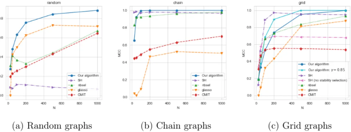
Figure 1-1: Comparison of different algorithms evaluated on MCC across (a) random, (b) chain and (c) grid graphs with 𝑝 = 100 and 𝑁 ∈ {25, 50, 100, 200, 500, 1000}. For each choice of 𝑝, 𝑁 for a given graph, results are shown as an average across 20 replications.
each tuning parameter and an edge is included in the estimated graph if it is selected often enough (we used 80%).
Discussion: Figure 1-1 compares the performance of the various methods based on MCC for random graphs, chain graphs and grid graphs. Figure 1-1(a) shows that our algorithm is able to offer a significant improvement for random graphs over competing methods. Also on chain graphs (Figure 1-1(b)) our algorithm is competitive with the other algorithms, with SH and nbsel performing comparably. For the grid graph (Figure 1-1(c)), for 𝑁 ≤ 500 SH with stability selection outperforms our algorithm with 𝛾 = 7/9. However, it is important to note that stability selection is a major advantage for the compared algorithms and comes at a significant computational cost. Moreover, by varying 𝛾 in our algorithm its performance can be increased and becomes competitive to SH with stability selection. Both points are discussed more in Appendix A.
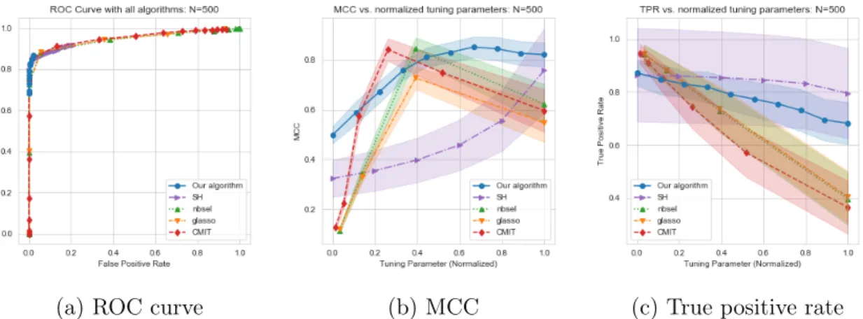
To evaluate the sensitivity of the various algorithms to their respective tuning parameters, we generate an ROC curve for each algorithm on random graphs with 𝑝 = 100 and 𝑁 ∈ {25, 50, 100, 200, 500, 1000}, of which 𝑁 = 500 is shown in Figure 1-2(a); see Appendix A for more details and plots. All algorithms perform similarly in terms of their ROC curves. Note that since our algorithm doesn’t have a true tuning
parameter, its false positive rate is upper bounded and thus it is impossible to get a full “ROC" curve. Figure 1-2(b) and (c) show the MCC and true positive rate (TPR) for each algorithm as a function of the tuning parameter normalized to vary between [0, 1]. Our algorithm is the least sensitive to variations in the tuning parameter, as it has one of the smallest ranges in both MCC and TPR (the 𝑦-axes) as compared to the other algorithms. Our algorithm also shows the smallest standard deviations in MCC and in TPR, showing its consistency across trials (especially compared to SH ). We here concentrate on TPR since the variation in FPR between all algorithms is small across trials. Taken together, it is quite striking that our algorithm with fixed 𝛾 generally outperforms methods with tuning parameters and stability selection.
1.4.2
Application to Financial Data
We now examine an application of our algorithm to financial data. The MTP2
constraint is relevant for such data, since the presence of a latent global market variable leads to positive dependence among stocks [33, 59]. We consider the daily closing prices for 𝑝 = 452 stocks that were consistently in the S& P 500 index from January 1, 2003 to January 1, 2018, which results in a sample size of 𝑁 = 1257. Due to computational limitations of stability selection primarily with CMIT, we performed
(a) ROC curve (b) MCC (c) True positive rate
Figure 1-2: (a) ROC curves, (b) MCC, and (c) true positive rate versus normalized tuning parameter for random graphs with 𝑝 = 100 and 𝑁 = 500 across 30 trials. The shaded regions correspond to ±1 standard deviation of MCC (TPR resp.) across 30 trials.
Method Modularity Coefficient Our Algorithm (𝛾 = 7./9.) 0.482
Slawski-Hein with stability selection 0.418 Neighborhood selection with stability selection 0.350 Graphical Lasso with stability selection 0.
Cross-validated graphical lasso 0.253 CMIT with stability selection -0.0088 CMIT with best hyperparameter -0.0085
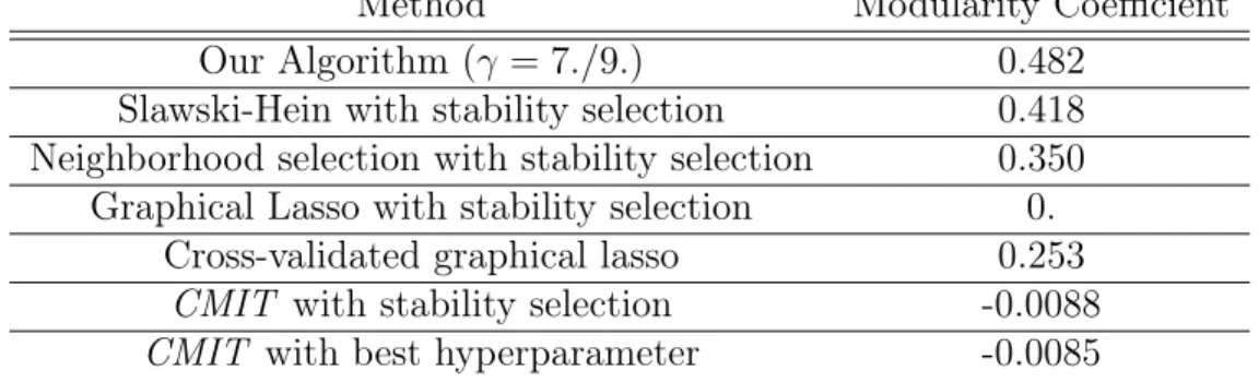
Table 1.1: Modularity scores of the estimated graphs; higher score indicates better clustering performance. For our algorithm we used the theoretically optimal value of 𝛾 = 7/9.
the analysis on the first 𝑝 = 100 of the 452 stocks.The 100 stocks are categorized into 10 sectors, known as the Global Industry Classification Standard (GICS) sectors. This dataset is gathered from Yahoo Finance and has also been analyzed in [49].
A common task in finance is to estimate the covariance structure between the log returns of stocks. Let 𝑆𝑗(𝑡) denote the closing price of stock 𝑗 on day 𝑡 and let 𝑋𝑗(𝑡) := log(︁𝑆𝑗(𝑡)/𝑆𝑗(𝑡−1))︁denote the log return of stock 𝑗 from day 𝑡 − 1 to 𝑡. Denoting by 𝑋 := (𝑋1, . . . , 𝑋100)𝑇 the random vector of daily log returns of the 100 stocks in
the data set, then our goal is to estimate the undirected graphical model of 𝑋. For this purpose, we treat the 1257 data points 𝑋(𝑡) := (𝑋(𝑡)
1 , . . . , 𝑋 (𝑡)
100) corresponding to
the days 𝑡 = 1, . . . , 1257 as i.i.d. realizations of the random vector 𝑋.
As in Section 1.4.1, we compare our method to SH, glasso (using both stability selection and cross-validation), nbsel and CMIT (using both stability selection and the hyperparameter with the best performance). Note that here we cannot assess the performance of the various methods using MCC since the graph structure of the true underlying graphical model is unknown. Instead, we assess each estimated graph based on its performance at grouping stocks from the same sector together. In particular, we consider the following metric that evaluates the community structure of a graph.
Modularity. Given an estimated graph 𝐺 := ([𝑝], 𝐸) with vertex set [𝑝] and edge set 𝐸, let 𝐴 denote the adjacency matrix of 𝐺. For each stock 𝑗 let 𝑐𝑗 denote the
in 𝐺. Then the modularity coefficient 𝑄 is given by 𝑄 = 1 2|𝐸| ∑︁ 𝑖,𝑗∈[𝑝] (︂ 𝐴𝑖𝑗 − 𝑘𝑖𝑘𝑗 2|𝐸| )︂ 𝛿(𝑐𝑖, 𝑐𝑗),
where 𝛿(·, ·) denotes the 𝛿-function with 𝛿(𝑖, 𝑗) = 1 if 𝑖 = 𝑗 and 0 otherwise.
The modularity coefficient measures the difference between the fraction of edges in the estimated graph that are within a sector as compared to the fraction that would be expected from a random graph. A high coefficient 𝑄 means that stocks from the same sector are more likely to be grouped together in the estimated graph, while a low 𝑄 means that the community structure of the estimated graph does not deviate significantly from that of a random graph. Table 1.1 shows the modularity scores of the graphs estimated from the various methods; our method using fixed 𝛾 = 7/9 outperforms all the other methods despite having no tuning parameter.
1.5
Discussion
In this section, we proposed a tuning-parameter free, constraint-based estimator for learning the structure of the underlying Gaussian graphical model under the constraint of MTP2. We proved consistency of our algorithm in the high-dimensional setting
without relying on an unknown tuning parameter. We further benchmarked our algorithm against existing algorithms in the literature with both simulated and real financial data, thereby showing that it outperforms existing algorithms in both settings. A limitation of our algorithm is that its time complexity scales as 𝑂(𝑝𝑑); it would be
interesting in future work to develop a more computationally efficient algorithm for graphical model estimation under MTP2. Another limitation is that our algorithm
is only provably consistent in the high-dimensional setting. However, the strong empirical performance of our algorithm as compared to existing algorithms is quite striking, given in particular its lack of a tuning parameter. To our knowledge, this is the first tuning-parameter free algorithm for structure recovery in Gaussian graphical models with consistency guarantees.
Chapter 2
Covariance Matrix Estimation under
Total Positivity for Portfolio Selection
2.1
Introduction
Given a universe of 𝑁 assets, what is the optimal way to select a portfolio? When "optimal" refers to selecting the portfolio with minimal risk or variance for a given level of expected return, then the solution, commonly known as the Markowitz optimal portfolio, depends on two quantities: the vector of expected returns 𝜇* and the covariance matrix of the returns Σ* [54]. In practice, 𝜇* and Σ* are unknown and must be estimated from historical returns data. Since Σ* requires estimating 𝑂(𝑁2)
different parameters while 𝜇* only requires estimating 𝑂(𝑁 ) different parameters, the main challenge lies in estimating Σ*. A naive strategy is to use the sample covariance matrix 𝑆 to estimate Σ*. However, this estimator is known to have poor properties [55, 67, 3, 38, 39], as can be seen by the following degrees-of-freedom argument (see also [19, Section 3.1]): as is common when daily or monthly returns are used, the number of historical data points 𝑇 is of the order of 1000 while the number of assets 𝑁 typically ranges between 100 and 1000. Since in this case 𝑇 ≪ 𝑁2, then only 𝑂(1)
effective samples are used to estimate each entry in the covariance matrix, making the sample covariance matrix perform poorly out-of-sample [47, 48, 19].
the high-dimensional setting, this problem has been widely studied in the statistics and financial economics literature. In the statistical literature, a number of estimators have been proposed based on banding or soft-thresholding the entries of 𝑆 [5, 4, 70, 10]. Such estimators, which are equivalent to selecting the covariance matrix closest to 𝑆 in Frobenius norm subject to the covariance matrix lying within a specified 𝐿1 ball, were
proven to be minimax optimal with respect to the Frobenius norm and spectral norm loss [10]. However, such estimators may not output a covariance matrix estimate that is positive definite, which is required for the Markovitz portfolio selection problem. Moreover, while such estimators are optimal in a minimax sense for the Frobenius and spectral norm loss, the loss actually relevant to measure the excess risk that results from using an estimate of Σ* instead of Σ* itself to compute the Markovitz portfolio is much different; see [19, Section 4.1] for details. Hence, the optimality results in [10] may no longer hold for selecting Markovitz portfolios.
Another reason to consider estimators beyond those in [5, 4, 70, 10] is that these methods do not exploit some of the structure that often holds in Σ*. In particular, the eigenspectrum of Σ* is often structured; we expect to find several important "directions" (i.e., eigenvectors) that well-approximate 𝑆. For example, if we believe that the capital asset pricing model (CAPM) model holds [6], then there should be one eigenvector in 𝑆 with large eigenvalue corresponding to the market. In other words, 𝑆 should be well-approximated by a rank one matrix. More generally, low-rank approximations of 𝑆 are advantageous statistically since these estimators have much smaller variance when the rank of the covariance matrix estimator is small1.
In practice, low-rank covariance estimates are based on explicitly provided factors [22, 24, 6], or data-driven factors learned by performing principal components analysis on 𝑆 [26, 36]. Another popular strategy to estimate Σ* is based on that assumption that the eigenvalues of Σ* are well-behaved, and exploit results from random matrix theory [18, 55]. In particular, various methods have regularized the eigenvalues of 𝑆 [47, 48, 19, 34, 16], which collectively can be regarded as particular instances of
1If the covariance matrix estimator has rank 𝑀 , then the effective number of parameters estimated
empirical Bayesian shrinkage [31, 47, 66]. Finally, a number of papers have proposed covariance estimators based on the assumption that the precision matrix is sparse. Such a constraint is motivated by the fact that a sparse precision matrix implies that the induced undirected graphical model associated with the joint distribution is sparse, which is desirable both for better interpretability and robustness properties [30].
In this section, we propose a new type of covariance estimator based on multivariate totally positive distributions of order 2 (MTP2), which exploits a new type of structure
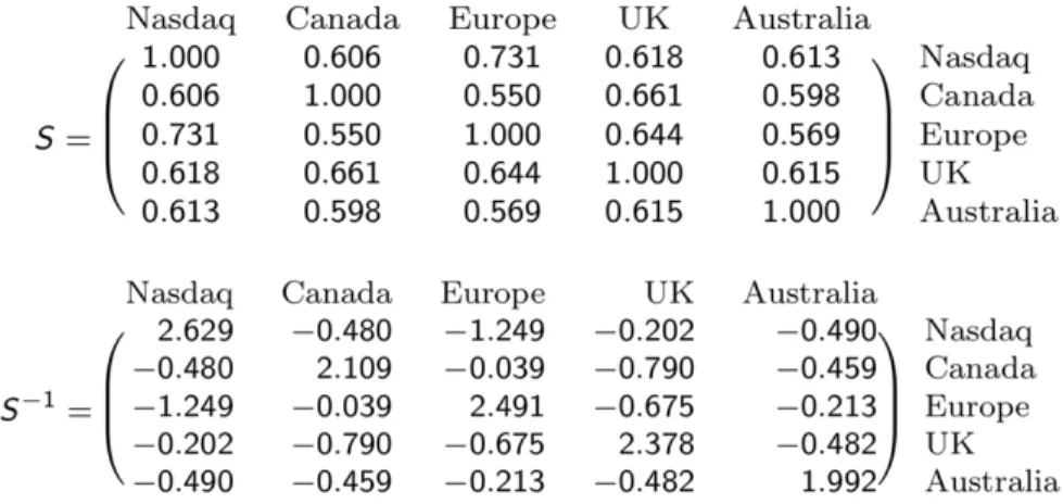
in the covariance matrix that previous methods have not considered. Furthermore, our method can be used "on top" of the previously mentioned methods. The structure we exploit is motivated by the observation that asset returns are often positively correlated since assets typically move together with the market. For example, if we look at the sample correlation matrix of the 2016 monthly returns of global stock markets, we see that all entries are positive in Fig. 2-1. Furthermore, when we invert this matrix, and examine the sample precision matrix, we see that all the off-diagonal
Figure 2-1: The sample correlation matrix of global stock markets taken from 2016 daily returns. Notice that the covariance matrix contains all positive entries and the precious matrix is an M-matrix which implies that the joint distribution is MTP2 (see
Section 2.3.2 for details).
entries are negative in Fig. 2-1. When a matrix has all negative off-diagonal entries, it is known as an M-matrix. When returns are distributed multivariate Gaussian, then the precision matrix being an M-matrix, implies that the joint distribution is MTP2 [42]. The fact that the precision matrix of the assets in Fig. 2-1 is an 𝑀 -matrix
is striking. A uniformly random covariance matrix with non-negative entries in R6 only has a precision matrix with non-positive off-diagonal entries with probability ≤ 10−6
. In Section 2.3.2 we show how to do estimation subject to the constraint that the joint distribution is MTP2, and further motivate studying MTP2 distributions in
Section 2.3.1.
The rest of the section is organized as follows: in Section 2.2 we mathematically detail the Markowitz portfolio problem, and review existing techniques for covariance estimation that we benchmark against in Section 2.4. In Section 2.3, we precisely define MTP2, motivate its usage for financial returns data, and describe how to do
covariance estimation under this constraint. Finally, in Section 2.4 we empirically compare our method with several competing methods on historical stock market data, and find that our method outperforms these other methods in terms of out-of-sample variance, i.e., risk.
2.2
Background
In this section, we mathematically detail the Markowitz portfolio selection problem as how it relates to covariance estimation, and review the literature on various covariance estimation techniques.
2.2.1
Notation
We assume that we have 𝑁 assets, which we index using the subscript 𝑖 and 𝑇 dates, which we index using the subscript 𝑡. The notation Cov represents the covariance matrix of a random vector.
We let 𝑟𝑖,𝑡 for 1 ≤ 𝑖 ≤ 𝑁 and 1 ≤ 𝑡 ≤ 𝑇 denote the observed return for asset 𝑖 at
date 𝑡. We let the vector 𝑟𝑡 denote the stacked vector 𝑟𝑡 := (𝑟1,𝑡, . . . , 𝑟𝑁,𝑡)𝑇, which
stands for the vector of all asset returns on day 𝑡. We let 𝜇𝑡:= ℰ [𝑟𝑡] and Σ𝑡:= Cov(𝑟𝑡):
2.2.2
Global Minimum Variance Portfolio
Typically in Markowitz portfolio theory, for a particular date 𝑡, given knowledge of 𝜇𝑡
and Σ𝑡 (the true expectation and covariance of the assets on day 𝑡), we want to assign
portfolio weights 𝑤 ∈ R𝑁 to our 𝑁 assets to solve the following optimization problem
min 𝑤 𝑤 𝑇Σ 𝑡𝑤, such that 𝜇𝑇𝑡𝑤 = 𝑅 with 𝑁 ∑︁ 𝑖=1 𝑤𝑖 = 1, (2.1)
for some parameter 𝑅, which represents the desired level of returns for the portfolio. The interpretation of this objective function is for some target return 𝑅, we want to assign weights 𝑤 to assets in our portfolio that minimizes the variance of the portfolio (which is given by 𝑤𝑇Σ
𝑡𝑤).
Although the above formulation of the Markowitz problem has a closed-form solution as a function of 𝜇𝑡 and Σ𝑡, for our purposeswe are not concerned with
estimating 𝜇𝑡 and only concerned with evaluating estimators of Σ𝑡. Thus we consider
the problem of estimating the global minimum variance (GMV) portfolio. This problem is formulated as min 𝑤 𝑤 𝑇Σ 𝑡𝑤, such that 𝑁 ∑︁ 𝑖=1 𝑤𝑖 = 1. (2.2)
We see in the above formulation, given 𝜇𝑡and Σ𝑡we are only concerned with assigning
portfolio weights 𝑤 to minimize the variance of the resulting portfolio (without regard to the expected return of the portfolio). This problem has the following analytical solution: 𝑤 = Σ −1 𝑡 1 1𝑇Σ−1 𝑡 1 (2.3) However, since we do not know the true Σ𝑡, in practice, we replace the unknown Σ𝑡
by an estimator ̂︁Σ𝑡 in the formula above, yielding a feasible portfolio ˆ 𝑤 := Σ̂︀ −1 𝑡 1 1𝑇 ̂︀ Σ−1𝑡 1. (2.4)
Estimating the global minimum variance portfolio is a widely used tactic to evaluate the quality of a covariance matrix estimator [32, 34], since it removes the need to estimate the vector of expected returns at the same time, which is not the focus of our work.
2.2.3
Covariance estimators
As discussed in the introduction, the sample covariance matrix is a poor estimator of the covariance. Furthermore, when 𝑁 > 𝑇 , where 𝑇 is the number of periods used to construct the sample covariance matrix (i.e. the sample size), then the sample covariance matrix is not even positive definite. Thus the sample covariance matrix cannot be inverted, which is needed in Formula 2.4. Although the sample covariance matrix is an unbiased estimator of the true covariance, it has very high variance and in the high-dimensional setting is not even consistent (e.g., the eigenvectors of 𝑆 do not even converge asymptotically to those in Σ* [55, 38, 67, 3, 39]). To obtain lower variance estimators of the covariance matrix, we make structural assumptions about the true covariance matrix that allows us to construct estimators that exploit this structure and lead to lower variance estimators with only a small increase in bias from the sample covariance matrix. We review several commonly used techniques for covariance matrix estimation in a financial context below.
2.2.4
Factor Models
A common modeling assumption behind a class of covariance matrix estimators is the factor model. In a factor model, there there are 𝐾 factors indexed by the subscript 𝑘 where 𝑓𝑘,𝑡 for 1 ≤ 𝑘 ≤ 𝐾 and 1 ≤ 𝑡 ≤ 𝑇 denotes the observed return for factor 𝑘
returns for day 𝑡. As factor model assumes that
𝑟𝑖,𝑡 = 𝛼𝑖+ 𝛽𝑖𝑇𝑓𝑡+ 𝑢𝑖,𝑡,
where 𝑢𝑖,𝑡 is the residual of asset 𝑖’s return with respect to the factor model
with ℰ [𝑢𝑖,𝑡] = 0. If we let 𝑢𝑡 = (𝑢1,𝑡, . . . , 𝑢𝑁,𝑡), then we can let Σ𝑓,𝑡 := Cov(𝑓𝑡) and
Σ𝑢,𝑡 := Cov(𝑢𝑡) denote the covariance of the factors and residuals on day 𝑡 respectively.
There are several different types of factor models
∙ A static factor model assumes that the covariance matrices Σ𝑢,𝑡 and Σ𝑓,𝑡 are
time-invariant, i.e. they do not depend on 𝑡.
∙ A exact factor model assumes that the covariance matrix Σ𝑢 is diagonal, but
an approximate factor model assumes that the covariance matrix Σ𝑢 only
has bounded 𝐿1 or 𝐿2 norm.
∙ A dynamic factor model relaxes the assumption that the covariance matrices Σ𝑢, Σ𝑓 are time-invariant and allows these matrices to depend on the date 𝑡.
If we let 𝐵 denote a matrix in R𝐾×𝑁 with 𝑖-th column given by 𝛽
𝑖, then the
covariance matrix Σ𝑟,𝑡 of the returns on day 𝑡 is given by Σ𝑓,𝑡, Σ𝑢,𝑡 and 𝐵 as follows:
Σ𝑟,𝑡 = 𝐵𝑇Σ𝑓,𝑡𝐵 + Σ𝑢,𝑡.
Most factor-model based covariance estimators derive estimates ̂︀Σ𝑓,𝑡 and ̂︀Σ𝑢,𝑡 for
Σ𝑓,𝑡 and Σ𝑢,𝑡 respectively. Then the estimator for Σ𝑟,𝑡 is given by
̂︀
Σ𝑟,𝑡 = ˆ𝐵𝑇Σ̂︀𝑓,𝑡𝐵 + ̂︀ˆ Σ𝑢,𝑡.
Intuitively, because the number of factors 𝐾 is generally small (and certainly much smaller than the number of assets 𝑁 , so 𝐾 << 𝑁 ), it is easier to obtain better estimates for Σ𝑓,𝑡 and Σ𝑢,𝑡 for the same number of samples, as compared to estimates
2.2.5
Covariance Estimators for Factor Models
We provide a high-level overview of several common factor-based covariance estimators that have been suggested for financial applications in the past.
∙ POET: is an estimator based on an approximate factor model proposed by [26]. The factors are determined by taking the top principal components of the {𝑟𝑡},
and the number of principal components used is determined by a data-driven criteria. The estimator of the covariance matrix of the factors ̂︀Σ𝑓 is given by
the sample covariance matrix of the principal components used. ̂︀Σ𝑢 is sparse
matrix that is obtained by applying thresholding to Diag(𝑆𝑢^), where 𝑆𝑢^ is the
sample covariance matrix of the residuals {ˆ𝑢𝑡}. This is a static estimator, since
the assumption is a static factor model.
∙ EFM: is an estimator based on an exact factor model. The factors are given by the commonly used Fama-French factors [23] (using either the one-factor model or the five-factor model using all 5 Fama-French factors). In either case, ̂︀Σ𝑓 is
given by the sample covariance matrix of the factors {𝑓𝑡} and ̂︀Σ𝑢 is given by
Diag(𝑆𝑢^).
∙ AFM-POET: is an estimator based on an approximate factor model. It is similar to EFM in that ̂︀Σ𝑓 is estimated similarly, except ̂︀Σ𝑢 is obtained by
thresholding 𝑆^𝑢, instead of simply considering the diagonal. The thresholding
scheme involves applying the POET method to the {ˆ𝑢} where the number of principal components used is set to 0 and the POET estimate of ̂︀Σ𝑢 is used.
This is a static estimator as well.
All of the estimators above are all static estimators and our estimator is also a static estimator. There have been several dynamic factor-model based estimators that account for the time-varying nature of Σ𝑓 and Σ𝑢, which is more realistic. However, as
our novel estimator is (currently) a static estimator, we want to benchmark it against other static estimators.
2.2.6
Shrinkage of eigenvalues
Another way to impose additional structure on the covariance matrix is assumptions on the behavior of the eigenvalues of the covariance matrix. These assumptions are more general than the factor model structure discussed above. Broadly speaking, the idea behind these assumptions is that the extreme eigenvalues of the sample covariance matrix are generally too large or too small [55, 3]. The solution is to assume that the eigenvalues of the true covariance matrix are more well-behaved, and to shrink the eigenvalues of the sample covariance matrix away from being too small or too large. The primary method that we review here is called linear shrinkage, as proposed in [47].
Linear Shrinkage
As proposed in [47], linear shrinkage considers the following eigendecomposition of the sample covariance matrix 𝑆:
𝑆 =
𝑁
∑︁
𝑖=1
𝜆𝑖𝑣𝑖𝑣𝑖𝑇,
where 𝜆𝑖 is the 𝑖-th eigenvalue of the matrix and 𝑣𝑖 is the corresponding eigenvector.
The linear shrinkage estimator assumes that the eigenvectors of 𝑆 and Σ are the same, but that the eigenvalues 𝛾𝑖 of Σ are shrunk versions of the eigenvalues 𝜆𝑖. In particular,
the linear shrinkage estimator sets 𝛾𝑖 = 𝜌𝜆𝑖 + (1 − 𝜌)¯𝜆, where ¯𝜆 is the average of
all of the eigenvalues of 𝑆 with a constant 0 ≤ 𝜌 ≤ 1. In [47], the authors derive an asymptotically efficient 𝜌 in terms of 𝑆 (the sample covariance matrix), 𝑁 (the dimension of matrix, i.e. the number of assets) and 𝑇 (the number of samples, i.e. days we consider). Then the linear shrinkage estimator is given by the following quantity: ̂︀ Σ𝐿𝑆 = 𝑁 ∑︁ 𝑖=1 𝛾𝑖𝑣𝑖𝑣𝑖𝑇. (2.5)
We also note that ̂︀Σ𝐿𝑆 can equivalent be expressed as
̂︀
Σ𝐿𝑆 = 𝜌𝑆 + (1 − 𝜌)¯𝜆𝐼𝑁, (2.6)
where 𝐼𝑁 is the identity matrix ∈ R𝑁 ×𝑁. This equality can be derived from
noticing that the 𝑣𝑖 are eigenvectors of the matrix expression on the right-hand side
of Equation 2.6 with eigenvalues given exactly by 𝛾𝑖. Thus we see that ̂︀Σ𝐿𝑆 is simply
a shrinkage of the sample covariance matrix towards a multiple of the identity, which can be motivated as viewing 𝐼𝑁 as a prior from a Bayesian point-of-view [47].
2.2.7
𝐿
1Regularization of the Precision Matrix
Another common technique to make covariance estimation easier is by assuming that the true unknown inverse covariance matrix (i.e., the precision matrix ) is sparse. That is,
‖𝐾‖0 :=
∑︁
𝑖̸=𝑗
𝐼(𝐾𝑖𝑗 ̸= 0) ≤ 𝜅 s.t. 𝐾 := Σ−1, (2.7)
where 𝜅 is an integer controlling the overall sparsity level of 𝐾. For multivariate Gaussian distributions, and more generally for transelliptical distributions [50], a sparse precision matrix implies that the induced undirected graphical model, which is a graph where nodes correspond to variables and edges correspond to non-zero correlations between variables, is sparse. This is desirable both for improved interpretability and robustness properties [30].
Unfortunately, maximizing the likelihood of the data subject to the cardinality constraint in Eq. (2.7) is computationally intractable as it involves solving a difficult combinatorial optimization problem. To make the optimization tractable, but still achieve sparsity, the graphical LASSO replaces the 𝐿0 constraint with an 𝐿1 constraint
[30]. In particular, the estimator for 𝐾 is given by solving the convex optimization problem,
ˆ
𝐾 = arg max
𝐾⪰0
log det 𝐾 − trace(𝐾𝑆) subject to ∑︁
𝑖̸=𝑗
where the objective function is the log-likelihood of the data, which is assumed to be distributed as a multivariate Gaussian, and 𝜆 is a hyperparameter controlling the sparsity level of ˆ𝐾 such that for larger 𝜆, ˆ𝐾 becomes sparser. For heavier-tailed data, the recent work of [50] has extended the graphical LASSO to handle heavier-tailed joint distributions.
2.3
MTP
2and our Method
So far, we have seen how different methods can make high-dimensional covariance estimation easier by either assuming low-dimensional structure, regularity in the eigenspectrum and/or sparsity in the unknown covariance matrix. Here, we exploit a new structure motivated by real asset returns data, namely that covariances between the returns of different assets are typically positive; see, for example, Fig. 2-1. Such behavior can partly be explained by the capital asset pricing model (CAPM). Recall that CAPM says that the return of stock 𝑖 can be modeled as,
𝑟𝑖 = 𝑟𝑓 + 𝛽𝑖(𝑟𝑚− 𝑟𝑓) 𝛽𝑖 ∈ R,
where 𝑟𝑓 is the risk-free rate of return, and 𝑟𝑚 is the market return. When 𝛽𝑖 and 𝛽𝑗
are positive, Cov(𝑟𝑖, 𝑟𝑗) is positive. Since 𝛽𝑖 is typically positive (since stocks go up
when the market goes up), this explains why the sample covariance matrix of stock market returns data contains nearly all positive entries2.
While CAPM is theoretically convenient, its simplicity comes at the expense of underfitting. In particular, there are often many (potentially unobserved) factors such as sector-level factors that drive returns. Identifying these important factors is an active area of research. For example, [22] extended CAPM to include three new factors and recently two more additional factors have been added [24]. However, since identifying relevant factors is challenging, we instead take a structure-free approach, and place constraints on the joint distribution such as requiring all entries in the
2The sample covariance matrix of 1000 assets (based on daily returns from 1980-2015) had over
covariance matrix to be positive to improve covariance estimation. In particular, we consider distributions that are MTP2.
Definition 2.3.1. A distribution 𝑝 on 𝒳 is multivariate totally positive of order 2 (MTP2) if
𝑝(𝑥)𝑝(𝑦) ≤ 𝑝(𝑥 ∧ 𝑦)𝑝(𝑥 ∨ 𝑦) for all 𝑥, 𝑦 ∈ 𝒳 ⊂ R𝑀,
where ∨, ∧ denote the coordinate-wise minimum and maximum respectively [27, 40]. Notice that Definition 2.3.1 is equivalent to 𝑝(𝑥) being log-supermodular. Log super-modularity has a long history in ecomomics, namely for comparative statics analysis [2, 14, 58], combinatorial optimization [62], and phylogenetics [72]. Theorem 2.3.2 below, which is proven in [28, Proposition 1], says that MTP2 implies positive
asso-ciation. Again, since we expect returns to be positively associated, this property of MTP2 distributions is desirable.
Theorem 2.3.2. If 𝑋 is MTP2, then 𝑋 is positively associated. That is, for any
non-decreasing functions 𝜑, 𝜓 : R𝑚↦→ R, Cov{𝜑(𝑋), 𝜓(𝑋)} ≥ 0.
While the MTP2 condition implies the desirable positive association structure
that we expect in real stock-market data, a natural question is why not simply do covariance estimation directly under the constraint that the covariances of returns be positive. These constraints make estimation computationally difficult (since a non-convex optimization problem must be solved) and for high-dimensional problems do not impose enough structure that a maximum-likelihood solution even exists [46].
To better motivate distributions satisfying Definition 2.3.1, we examine latent tree models in Section 2.3.1, which includes single-factor models such as CAPM. Since latent trees models imply MTP2 for multivariate Gaussian distributions, we discuss
several implications of this fact for improved covariance estimation in what follows.
2.3.1
Latent Tree Models
A powerful framework to model complex data such as stock-market returns data is through latent tree models. A latent tree is an undirected graph such that any
two nodes are connected by a unique path, where nodes represent random variables that may or may not be observed. For financial applications, latent trees have been used for unsupervised learning tasks, such as clustering stocks together and learning latent graphical structures for asset returns [12, 53]. Many factor models, such as the single-factor model assumed in CAPM, are also examples of latent trees; see Fig. 2-2 for concrete examples. The following theorem, which follows from [46, Theorem 5.4], shows that if we believe the data is generated from a latent tree, then assuming that the joint distribution of all the variables is MTP2 is a necessary condition.
Theorem 2.3.3. Suppose 𝐺 is an undirected tree and 𝑋 ∈ R𝑀 is multivariate
Gaussian and Markov respect to 𝐺. That is, the joint distribution of 𝑋 factorizes as
𝑝(𝑋) =
𝑀
∏︁
𝑖=1
𝑝(𝑋𝑖 | Pa𝐺(𝑋𝑖)),
where Pa𝐺(𝑋𝑖) denotes the parents of node 𝑋𝑖 in 𝐺. Then, |𝑋| is MTP2 and any
marginal distribution of 𝑋 is MTP2. If the covariance matrix of 𝑋 contains all positive
entries, then 𝑋 is MTP2 and any marginal of 𝑋 is MTP2.
Any distribution such that |𝑋| is MTP2 is called signed MTP2. While there are
methods to do estimation when 𝑋 is signed MTP2 [46], in this section we focus on
when 𝑋 is MTP2 since for latent trees, a covariance matrix with all positive entries
implies 𝑋 is MTP2. While Theorem 2.3.3 says that MTP2 distributions over trees are
closed under marginalization, this closure property holds more generally for MTP2
distributions over arbitrary graphs [42]. Hence, even if we do not observe certain factors, if we simply assume that the factors and observed random variables form a latent tree or are MTP2, then the marginal joint distribution of the observables (e.g.,
the returns of each asset) is still MTP2. Unfortunately, we often do not know the
structure of the latent tree, and trying to learn the structure from data is NP-hard [13]. Instead, we show in Section 2.3.2 how to do covariance estimation subject to an MTP2 constraint, which again is a necessary but not sufficient condition for the
joint distribution of the returns to be generated from a latent tree for the multivariate Gaussian case. By removing the constraint that the joint distribution factorizes
IBM Intel IBM Intel Market Oil Cost Sillicon Cost Coke
Coke Pepsi GM Pepsi GM
Sugar Cost
Figure 2-2: Shaded nodes represent factors that are potentially unobserved, and unshaded nodes are the observed returns of different companies. The left hand figure represents a simple model where we think the market drives the returns of all stocks as in CAPM. The right hand figure represents a more complicated latent tree where we believe that there are latent sector-level factors driving the returns of different assets.
according to a latent tree, we show in Section 2.3.2 that we can find an MTP2
covariance estimator by solving a simple convex optimization problem. Furthermore, working only under an MTP2 constraint allows us to model richer graphical structures
[21]. Since the MTP2 constraint is already quite restrictive, the added variance of
modeling graphical structures beyond latent trees is not large, and may in fact be better than the bias of assuming that the joint distribution is generated exactly from a latent tree.
2.3.2
Multivariate Gaussian Returns
For multivariate Gaussian distributions, a necessary and sufficient condition for a distribution to be MTP2 is that the precision matrix 𝐾 := Σ−1 is an M-matrix. That
is, 𝐾𝑖𝑗 ≤ 0 for all 𝑖 ̸= 𝑗 or, equivalently, if all partial correlations are nonnegative. [42].
Following [46], we consider the maximum likelihood estimator (MLE) of 𝐾 subject to 𝐾 being an M-matrix.
Recall that the log-likelihood ℒ of 𝐾 given data 𝐷 := {𝑟𝑡}𝑇𝑡=1 i.i.d.
∼ 𝑁 (0, 𝐾) is, up to additive and multiplicative constants, given by
where 𝑆 := 𝑇1 ∑︀𝑇
𝑡=1𝑟𝑡𝑟 𝑇
𝑡 is the sample covariance matrix with 𝑆 ∈ R𝑁 ×𝑁. The MLE of
𝐾 is obtained by maximizing ℒ(𝐾; 𝐷) over the set of all positive semidefinite matrices, which equals 𝑆−1 when 𝑁 ≤ 𝑇 (i.e. the dimension of the matrix is less than the number of samples). Note that the MLE only exists when 𝑁 ≤ 𝑇 since 𝑆 must be invertible. Remarkably, if we add the constraint that 𝐾 is an M-matrix (i.e., that the distribution is MTP2) and maximize the likelihood, that is solve
ˆ
𝐾 = arg max
𝐾⪰0 log det 𝐾 − trace(𝐾𝑆) subject to 𝐾𝑖𝑗 ≤ 0 ∀𝑖 ̸= 𝑗, (2.10)
then a unique maximum exists with probability one when 𝑇 ≥ 2 for any dimension 𝑁 [64, 46]. The fact that a unique solution exists for Eq. (2.10) for any 𝑁 suggests that an MTP2 constraint adds considerable structure and regularization for covariance
estimation.
We now discuss several desirable properties of the optimization problem in Eq. (2.10). The first is that Eq. (2.10) is a convex optimization problem since the objective and constraints are concave. Hence, computationally efficient coordinate-descent solvers can find ˆ𝐾 [46, Algorithm 1]. Another desirable property is that ˆ𝐾 is sparse, namely ˆ𝐾 contains many zero entries [46, Corallary 2.9]. Recall that for multivariate Gaussian distributions, the sparsity pattern of ˆ𝐾 is in 1-1 correspon-dence with an induced undirected graphical model, namely a graph with edges for all non-zero ˆ𝐾𝑖𝑗 entries. Hence, for high-dimensional problems, having sparsity in 𝐾
adds regularization and reduces the variance of the estimator because the underlying graphical model is low-dimensional i.e. contains few edges. One immediate advantage of Eq. (2.10) over methods that explicitly add sparsity-inducing 𝐿1 penalties such
as the graphical LASSO [30] discussed in Section 2.2.7, is that Eq. (2.10) does not require any tuning parameters to achieve sparsity.
2.3.3
Future Work:
Accommodating Heavy-Tailed Returns
Data
We discuss the implications of the practical fact that real-life returns have heavier tails than multivariate Gaussians. This is a problem because the optimal Markowtiz portfolio weights given in Equation 2.3 implicitly assumes returns are multivariate Gaussian. Furthermore, many statistical estimators are based on the assumption that the data are multivariate Gaussian. To make returns “look” more multivariate Gaussian, practioners often look at log returns. Unfortunately, log returns are still typically not multivariate Gaussian, which is a potential issue since our estimator in Section 2.3.2 is based heavily on Gaussianity. Instead of trying to find a better transformation than the log-transform to get Gaussianity for heavier-tailed returns data, we propose in future work to replace the sample covariance matrix with the Kendall’s tau covariance matrix estimator in Eq. (2.10). Before going in any more depth about this estimator, we first specify the precise problem we would like to solve.
We would like to find functions 𝑓1, · · · , 𝑓𝑀 such that (𝑓1(𝑋1), · · · , 𝑓𝑀(𝑋𝑀)) is
multivariate Gaussian with covariance matrix Σ𝑓. If we could find such functions,
then we could use our MTP2 estimator in Eq. (2.10) on this tranformed data. Again, practitioners typically set 𝑓𝑖(𝑥) = log(𝑥), and use any of the previously mentioned
covariance estimators on this log-transformed data. However, the log transformed data still might not be multivariate Gaussian.
The following theorem, which is proven in [50], shows that Kendall’s tau provides a non-parametric estimate of Σ𝑓. That is, each 𝑓𝑖 only needs to be monotonically
increasing for Kendall’s tau to converge asymptotically to Σ𝑓.
Theorem 2.3.4. Suppose there exists monotonically increasing functions 𝑓1, · · · , 𝑓𝑀
such that (𝑓1(𝑋1), · · · , 𝑓𝑀(𝑋𝑀)) is multivariate Gaussian with covariance matrix Σ𝑓.
Then, sin(𝜋2𝜏 ) → Σˆ 𝑓, where
ˆ 𝜏𝑖𝑗 = 1 (︀𝑇 2 )︀ ∑︁ 1≤𝑡≤𝑡′≤𝑇 sign(𝑋𝑖𝑡− 𝑋𝑖𝑡′) sign(𝑋𝑗𝑡− 𝑋𝑗𝑡′).